```{r setup,echo=FALSE}
require(Hmisc)
require(qreport)
require(ggplot2)
```
# Measures of Evidence
## General
### Indirect
* If we assume suspect A did not commit the crime, his behavior in the following days is very unusual, so let's act as if A is the perpetrator.
* We have only two suspects. The likelihood that suspect A committed the crime is small, so we turn attention to suspect B even though we don't know the chance that B did it.
### Direct
* A police officer witnessed suspect B committing the crime (no analogy in drug development)
* Based on DNA, fingerprint, and motive, the probability that suspect B committed the crime is 0.98
* Note: it is impossible to assign an absolute probability that the suspect is guilty without having a pre-investigation prior probability of guilt (but one can compute _relative_ guilt ratios without this)
## Frequentist
* p-value: P(data as or more extreme than what we observed \| H<sub>0</sub> true)
* Probability here = long-run relative frequency
* NHST: null hypothesis significance test
* Backwards in time/information flow
* Doesn't relate to clinical significance (@mar16und)
* Requires arbitrary multiplicity adjustments because considers what _could_ have happened
* Don't want to know P(batter who just got a hit is left-handed)
#### Analogy to Diagnostic Testing
* Sensitivity: P(T+ \| D+) [power]
* Specificity: P(T- \| D-) [1 - type I "error"]
* Bayes' rule: P(D+\|T) = P(T\|D+) P(D+) / P(T)<br>=sens x prevalence / (sens x prev + (1-spec)(1-prev))
* High sens and spec easily overcome by low prev
* sens and spec vary with patient
* What _could have happened but didn't_ important, just as need to correct p-values for multiple data looks in sequential RCTs
+ need to correct sens and spec for verification/referral bias
+ after using Bayes' rule to get P(D\|T) the corrections cancel out
* P(D\|T) is directly actionable and defines its own error risk
+ P(cancer) = 0.8 implies P(unnecessary biopsy)=0.2
#### Back to p-values
* p="degree to which the data are embarrassed by the null hypothesis" (@max04dat)
* Only can provide evidence against H<sub>0</sub>, **never** evidence in favor of something
* Efficacy inferred from having much evidence against "no efficacy"
* If set α=0.05, type I assertion probability never reduces even as n→∞
* Likelihood school of inference: both type I and type II assertion probabilities → 0
* Type I α perhaps useful at study design stage
* After study completes, can only know if type I "error" was committed if true effect is exactly zero
+ but then would not have needed the study
* Type I assertion prob is a long-run operating characteristic for sequence of studies
* Consider sequence of p-values from them
+ type I prob α means P(p-value < α \| zero effect) = α
* Neither p-value nor α are probs of a decision error
* p-value = P(data more extreme than ours \| no effect)
+ not a false + prob for experiment at hand
+ that would require a prior
::: {.panel-tabset .quoteit}
### Quotes
### Deming
A basic difficulty for most students is the proper formulation of the alternatives H<sub>0</sub> and H<sub>1</sub> for
any given problem and the consequent determination of the proper critical region (upper tail, lower tail, two-sided). ...<br><br>_Comment_. Small wonder that students have trouble. They may be trying to think. ...<br><br>_More on the teaching of statistics_. Little advancement in the teaching of statistics is possible, and little hope for statistical methods to be useful in the frightful problems that face man today, until the literature and classroom be rid of terms so deadening to scientific enquiry as null hypothesis, population (in place of frame), true value, level of significance for comparison of treatments, representative sample.<br><br>
Statistical significance of B over A thus conveys no knowledge, no basis for action.---@dem75pro
### Rozeboom
The null-hypothesis significance test treats 'acceptance' or 'rejection' of a hypothesis as though these were decisions one makes. But a hypothesis is not something, like a piece of pie offered for dessert, which can be accepted or rejected by a voluntary physical action. Acceptance or rejection of a hypothesis is a cognitive process, a degree of believing or disbelieving which, if rational, is not a matter of choice but determined solely by how likely it is, given the evidence, that the hypothesis is true. -- @roz60fal quoted by [EJ Wagenmakers and Q Gronau](https://www.bayesianspectacles.org/redefine-statistical-significance-xvii-william-rozeboom-destroys-the-justify-your-own-alpha-argument-back-in-1960)
### Kruschke & Liddell
... Another concern is that Bayesian methods do not control error rates as indicated by p values. ... This concern is countered by repeated demonstrations that error rates are extremely difficult to pin down because they are based on sampling and testing intentions. --- @kru17bay
### Berry
If the design were unknown, then it is not possible to calculate a P value. ... Every practicing statistician must deal with data from experiments the designs of which have been compromised. For example, clinical trials are plagued with missing
data, patients lost to follow-up, patients on the wrong dosing schedule, and so forth. Practicing statisticians cannot take the unconditional perspective too seriously or they cannot do statistics! --- @ber87int
:::
#### Other Subtle Problems with p-values {-}
* Proof by contradiction doesn't directly apply outside of non-fuzzy logic
* p is not P(results as impressive as ours \| H<sub>0</sub>)<br>It is P(more impressive)
* Computed under assumption of zero treatment effect; doesn't formally entertain harm
* Can argue that H<sub>0</sub> is **always** false
* NHST entails fixing n; many studies stop with p=0.06 when could have added 20 more subjects
+ frequentist approach to sample size re-estimation requires discounting of data from first wave of subjects
* See also @nuz14sci
::: {.panel-tabset .quoteit}
### Quotes
### Cohen
The following is almost but not quite the reasoning of null hypothesis rejection:<br><br>
If the null hypothesis is correct, then this datum (D) can not occur.<br>
It has, however, occurred.
Therefore the null hypothesis is false.<br><br>
If this were the reasoning of H<sub>0</sub> testing, then it would be formally correct. ... But this is
not the reasoning of NHST. Instead, it makes this reasoning probabilistic, as follows: <br><br>
If the null hypothesis is correct, then these data are highly unlikely.<br>
These data have occurred.<br>
Therefore, the null hypothesis is highly unlikely.<br><br>
By making it probabilistic, it becomes invalid. ... the syllogism becomes formally incorrect
and leads to a conclusion that is not sensible:<br><br>
If a person is an American, then he is probably not a member of Congress. (TRUE, RIGHT?)<br>
This person is a member of Congress.<br>
Therefore, he is probably not an American. (Pollard & Richardson, 1987)<br>
.. The illusion of attaining improbability or the Bayesian Id's wishful thinking error ...<br><br><br>
Induction has long been a problem in the philosophy of science. Meehl (1990)
attributed to the distinguished philosopher Morris Raphael Cohen the saying
"All logic texts are divided into two parts. In the first part, on
deductive logic, the fallacies are explained; in the second part, on
inductive logic, they are committed." --- @coh94ear
### Briggs
A person is interested in a probability model. But guided by the philosophy of p-values, he asks no questions about this model, and instead asks what is the probability, given the data and some other model, which is not the model of interest, of seeing an ad hoc statistic larger than some value. (Any change in a model produces a different model.) Since there are an infinite number of models that are not the model of interest, and since there are an infinite number of statistics, the creation of p-values can go on forever. Yet none have anything to say about the model of interest.<br><br>
Why? Fisher (1970) said: "Belief in null hypothesis as an accurate representation of the population sampled is confronted by a logical disjunction: Either the null is false, or the p-value has attained by chance an exceptionally low value."<br><br>
Fisher's "logical disjunction" is evidently not one, since the either-or describes different propositions. A real disjunction can however be found: Either the null is false and we see a small p-value, or the null is true and we see a small p-value. Or just: Either the null is true or it is false and we see a small p-value. Since "Either the null is true or it is false"" is a tautology, and is therefore necessarily true, we are left with, "We see a small p-value." The p-value casts no light on the truth or falsity of the null.<br><br>
Frequentist theory claims, assuming the truth of the null, we can equally likely see any p-value whatsoever. And since we always do (see any value), all p-values are logically evidence for the null and not against it. Yet practice insists small p-value is evidence the null is (likely) false. That is because people argue: For most small p-values I have seen in the past, the null has been false; I now see a new small p-value, therefore the null hypothesis in this new problem is likely false. That argument works, but it has no place in frequentist theory (which anyway has innumerable other difficulties).<br><br>
Any use of p-values in deciding model truth thus involves a fallacy or misunderstanding. This is formally proven by Briggs (2016, chap. 9), a work which I draw from to suggest a replacement for p-values, which is this. Clients ask, "What's the probability that if I know X, Y will be true?" Instead of telling them that, we give them p-values. --- @bri17sub
### Cohen
The nil hypothesis is always false. Tukey (1991) wrote that "It is foolish to ask 'Are the effects of A and B different?' They are always different---for some decimal place". Schmidt (1992) ... reminded researchers that, given the fact
that the nill hypothesis is always false, the rate of Type I errors is 0%, not 5%, and that only Type II errors can be made. --- @coh94ear
### Feinstein
(The use of p-values) is a lamentable demonstration of the credulity with which modern scientists will abandon biologic wisdom in favor of any quantitative ideology that offers the specious allure of a mathematical replacement for sensible thought. --- @fei77cli
### Oakes
It is incomparably more useful to have a plausible range for the value of a parameter than to know, with whatever degree of certitude, what single value is untenable. --- @oak86sta
:::
#### Issues with Confidence Limits
* CLs have only long-term interpretations and give false impression that all values within the interval are equally likely
* Cannot control which interval for which you want a probability statement
::: {.panel-tabset .quoteit}
### Quotes
### Wagemakers
I see that the 0.95 confidence interval for the mean blood pressure difference is [2,7]. But I want to know the confidence I should have in it being in the interval [0,5] and you're telling me it can't be computed with frequentist confidence intervals? --- @wag17bay1
### Gelman & Hennig
The worry is that, when data are weak and there is strong prior
information that is not being used, classical methods can give answers that
are not just wrong---that's no dealbreaker, it's accepted in statistics
that any method will occasionally give wrong answers---but clearly wrong;
wrong not only just conditional on the unknown parameter but also
conditional on the data. Scientifically inappropriate conclusions. That's
the meaning of 'poor calibration.' Even this, in some sense, should not
be a problem---after all, if a method gives you a conclusion that you know
is wrong, you can just set it aside, right?---but, unfortunately, many
users of statistics consider to take p < 0.05 or p < 0.01 comparisons
as 'statistically significant' and to use these as a motivation to accept
their favored alternative hypothesis. This has led to such farces, in recent
claims, in leading psychology journals that various small experiments
have demonstrated the existence of extra-sensory perception or huge
correlations between menstrual cycle and voting, and so on. --- @gel17bey
### Hadler
So what happened with the development of efficacy measures
is we developed a whole new field called biostatistics. It had been sort of
an orphan corner of mathematics until the Kefauver-Harris Amendments, and there
had been extremely important advances in how do you study efficacy of drugs.
Most of it devolves down to whether or not you're likely to see
a benefit more than chance alone would predict. But _how likely_ and
_how much_ benefit was left for some free-floating kind of notion by the
FDA. So _any_ benefit in essence, more than any toxicity in essence, would lead to
licensure. That has led to what I call "small effectology."<br><br>
Nortin Hadler, [Interviewed](http://www.wbur.org/onpoint/2016/03/29/doctor-patient-care-aca-obamacare) by Tom Ashbrook _On Point_, WBUR radio, 2016-03-29, 15:26
### FH
p-value: the chance that someone else's data are more extreme than mine if H<sub>0</sub> is true, not the chance that H<sub>0</sub> is true given my data<br><br>
Aside from ignoring applicable pre-study data, the p-value is at least monotonically related to what we need. But it is not calibrated to be on a scale meant for optimum decision making.
### Kruschke & Liddell
The criterion of p < .05 says that we should be willing to tolerate a 5% false alarm rate in decisions to reject the null value. In general, frequentist decision rules are driven by a desire to limit the probability of false alarms. The probability of false alarm (i.e., the p value) is based on the set of all possible test results that might be obtained by sampling fictitious data from a particular null hypothesis in a particular way (such as with fixed sample size or for fixed duration) and examining a particular suite of tests (such as various contrasts among groups). Because of the focus on false alarm rates, frequentist practice is replete with methods for adjusting decision thresholds for different suites of intended tests. ...<br><br>
Bayesian decisions are not based on false alarm rates from counterfactual sampling distributions of hyopthetical data. Instead, Bayesian decisions are based on the posterior distribution from the actual data. --- @kru17bay
### Goodman
... Neyman and Pearson outline the price that must be paid to enjoy the purported benefits of objectivity: We must abandon our
ability to measure evidence, or judge truth, in an individual experiment. ... Hypothesis tests are equivalent to a system of justice that is not concerned with which individual defendent is found guity or innocent (that is , "whether each separate hypothesis is true or false") but tries instead to control the overall number of incorrect verdicts (that is, "in the long run of experience, we shall not often be wrong"). Controlling mistakes in the long run is a laudable goal, but just as
our sense of justice demands that individual persons be correctly judged, scientific intuition says that we should try to draw the proper conclusions from individual studies. --- @goo99tow
:::
### Computing p-values Using Simulation
* Simulations help one to grasp theory
* One-sample problem for a normal mean μ
* Single-arm study, μ > 0 denotes efficacy
* Assume σ = 1
* n=30, true μ = 0.3
* Simulate 100,000 studies
* Also compute P(result approx. **as** impressive as observed \| μ = 0)<br>within window of width 0.1
```{r pval}
n <- 30
set.seed(1)
y     <- rnorm(n, 0.3, sd=1)            # generate data
ybar  <- mean(y)                        # observed mean
ucl   <- ybar + qnorm(0.95) / sqrt(30)  # upper C.L.
# Run 100,000 studies and compute their sample means:
repeated.ybar <- rnorm(100000, 0, sd=sqrt(1/30))
# TRUE/FALSE variables are converted to 1/0 when taking the mean
# This is an easy way to compute a proportion
p     <- mean(repeated.ybar >= ybar)
pa    <- mean(repeated.ybar >= ybar & repeated.ybar <= ybar + 0.1)
repeated.ucl <- repeated.ybar + qnorm(0.95) / sqrt(30)
cover <- mean(repeated.ucl >= 0)
cat('Observed mean           : ', round(ybar, 3), '\n',
    'Upper 0.95 1-sided CL   : ', round(ucl, 3), '\n',
    'One-sided p-value       : ', round(p, 4), '\n',
    'Exact p-value           : ', round(1 - pnorm(ybar, 0, sd=1/sqrt(30)),
                                  4), '\n',
    'Confidence coverage     : ', round(cover, 4), '\n',
    'P(Approx. as impressive): ', round(pa, 4), '\n',
    sep='')
```
* Modify simulation for 2 data looks, with stopping rule
* First look after n=15 with nominal type I error 0.05
* Stop study if mean exceeds corresponding cutoff
* Otherwise use mean of n=30 as final estimate and basis for test
* Compute two 'nominal' p-values and then the actual p-value under the stopping rule
* Assumptions exposed
+ intended look is actually carried out
+ look is ignored if p > 0.05
```{r pval2}
set.seed(1)
# Make first look
y1 <- rnorm(n / 2, 0.3, sd=1)
ybar1 <- mean(y1)
# Make second look
y2 <- rnorm(n / 2, 0.3, sd=1)
ybar2 <- mean(c(y1, y2))      # combine to get n=30
ybar.at.stop  <- ifelse(ybar1 * sqrt(15) >= qnorm(0.95), ybar1, ybar2)
ybar.at.stopb <- ifelse(ybar1 * sqrt(15) >= qnorm(0.975),ybar1, ybar2)
# Run 100,000 studies.  For each get mean with n=15 and 30 and apply the same stopping rule
repeated.ybar1 <- rnorm(100000, 0, sd=sqrt(1/15))
# Compute overall mean with n=30:
repeated.ybar2 <- (repeated.ybar1 + rnorm(100000, 0, sd=sqrt(1/15))) / 2
# Compute estimate of mean at last look, using 2 stopping rules
repeated.ybar  <- ifelse(repeated.ybar1 * sqrt(15) >= qnorm(0.95),
                         repeated.ybar1, repeated.ybar2)
repeated.ybarb <- ifelse(repeated.ybar1 * sqrt(15) >= qnorm(0.975),
                         repeated.ybar1, repeated.ybar2)
pval1          <- mean(repeated.ybar1 >= ybar1)  # ordinary p-value n=15
pval2          <- mean(repeated.ybar2 >= ybar2)  # ordinary p-value n=30
# P-value accounting for multiple looks using alpha=0.05
pval           <- mean(repeated.ybar  >= ybar.at.stop)
# Same using alpha=0.025
pvalb          <- mean(repeated.ybarb >= ybar.at.stopb)

cat('Sample mean at first look     :', round(ybar1, 3), '\n',
    'Sample mean at end            :', round(ybar2, 3), '\n',
    'Nominal p-value at n=15       :', round(pval1, 4), '\n',
    'Nominal p-value at n=30       :', round(pval2, 4), '\n',
    'p-value accounting for looks  :', round(pval,  4), '\n',
    'p-value " " with alpha=0.025  :', round(pvalb, 4), '\n', sep='')
```
* True p-value accounting for 2 looks > simple p-value
* True p-value smaller if used instead α = 0.025
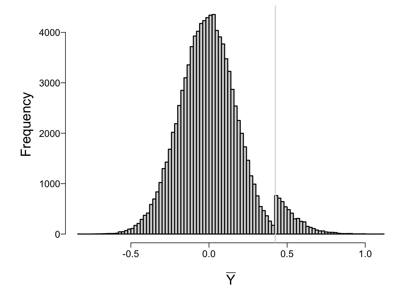
* Sampling distribution for the sample mean under our 0.05 stopping rule has a discontinuity at the value of the mean that would cause early stopping
* Difficult to derive and use the true sampling distribution under multiple looks; most statisticians pretend only 1 look done
* Bayesian inference doesn't concern itself with sampling distributions
```{r ymeanstop}
#| fig.cap: 'Sampling distribution of final estimate of the mean in a two-stage sequential single arm trial, under the null hypothesis'
spar(bty='l')
hist(repeated.ybar, nclass=100, xlab=expression(bar(Y)), main='')
abline(v=qnorm(0.95) / sqrt(15), col=gray(.85))
```
## Bayesian
::: {.quoteit}
This form (probability of unknown given what is known) has enormous benefits. It is in plain language; specialized training is not needed to grasp model statements ... Everything is put in terms of observables. The model is also made prominent, in the sense that it is plain there is a specific probability model with definite assumptions in use, and thus it is clear that answers will be different if a different model or different assumptions about that model are used ... --- @bri17sub
:::
* Relative changes in evidence are functions only of data
* No absolute truths
* Final evidence quantified on an absolute scale given pre-data anchor
* Bayes' theorem: movement of prior belief to current belief
* Full conditioning on observables
* Does not condition on unknowables
* Probability statements forward in time/information so have meaning out of context
* Multiple looks/stopping rule not relevant
* Helpful in understanding how a Bayesian might cheat:
+ change prior after seeing data
+ hiding data, e.g. P(efficacy) = 0.95, enroll more subjects, P(efficacy) = 0.93, report previous look as final
#### Example Frequentist Result
* Difference in mean SBP between treatments A, B = 6mmHg
* p=0.01, 0.95 CL [3,9]
* An event (?) (of ≥ 6 mmHg) of low probability has been witnessed if A=B
#### Corresponding Bayesian Result
* Use a normal prior satisfying
+ pre-study chance of worsening BP is 0.5
+ pre-study chance of a large (≥ 10mmHg) improvement in BP is 0.1
* Posterior mean BP reduction 5mmHg
* 0.95 credible interval: [2.5, 8]
* P(reduction in BP) = 0.97
* P(reduction ≥ 2mmHg) = 0.9
* P(similarity) = P(\|difference\| ≤ 2mmHg) easy to compute
#### Updating of Posterior in Sequential Trials
* Coin flipping, prior is beta(10,10) favoring fairness
* 100 tosses, update posterior every 10 tosses
* After n tosses with y heads, posterior is beta(Y + 10, n - y + 10)
* Repeat for beta(5,5) and beta(20,20) priors
* Click on the legend to hide or display results for the 3 priors<br><small>Double-click to show only one set</small>
```{r beta}
#| fig.cap: "Prior distribution (blue) and posterior distributions as the trials progress (darkness of lines increases). The final posterior at N=100 is in red, when there were 53 heads tossed."
require(plotly)
x <- seq(0, 1, length=200)
p <- plot_ly(width=800, height=500)
for(ab in c(10, 5, 20)) {
    set.seed(1)
    alpha <- beta <- ab
    lg  <- paste0('α=', alpha, ' β=', beta)
    vis <- if(ab == 10) TRUE else 'legendonly'
    Y   <- 0
    # Plot beta distribution density function
    p <- p %>% add_lines(x=~x, y=~y, hoverinfo='none', visible=vis,
        line=list(color='blue'),
        name=paste0('Prior:', lg), legendgroup=lg,
        data=data.frame(x=x, y=dbeta(x, alpha, beta)))

    for(N in seq(10, 100, by=10)) {
        Y <- rbinom(1, 10, 0.5)  # 10 new tosses
        # Posterior distribution updated
        alpha <- alpha + Y
        beta  <- beta + 10 - Y
        p <- p %>% add_lines(x=~x, y=~y, hoverinfo='none', visible=vis,
            name=paste0('N=', N, ' ', lg), legendgroup=lg,
            line=list(color=if(N < 100) 'black' else 'red',
                opacity=if(N < 100) .95 - N / 120 else 1,
                width=N * 2 / 100),
            showlegend=FALSE,
            data=data.frame(x=x, y=dbeta(x, alpha, beta)))
      }
    }
p %>% layout(shapes=list(type='line', x0=.5, x1=.5, y0=0, y1=9, opacity=.2),
        xaxis=list(title='θ'), yaxis=list(title=''))
```
### Alternative Take on the Prior
* Can also think of the prior as augmenting or reducing the effective sample size (@wie19qua)
* Consider a skeptical prior
* Effectively ignoring some of the sample
* When the data are normally distributed with mean $\mu$ and variance $\sigma^2$, $\overline{Y}$ is normal with mean $\mu$ and variance $\frac{\sigma^{2}}{n}$
* When the prior is also Gaussian but with mean $\mu_{0}$ and variance $\sigma^{2}_{0}$, the posterior distribution of $\mu$ is normal with the following variance and mean, respectively, if we let the _precision_ of the prior $\tau = \frac{1}{\sigma^{2}_{0}}$:
* $\sigma^{2}_{1} = (\tau + \frac{n}{\sigma^{2}})^{-1}$
* $\mu_{1} = \sigma^{2}_{1} (\mu_{0} \tau + \frac{n \overline{Y}}{\sigma^{2}})$
* Consider special case where the data variance $\sigma^2$ is 1 and the prior mean is zero; then the posterior variance and mean of $\mu$ are:
* $\sigma^{2}_{1} = (n + \tau)^{-1}$
* $\mu_{1} = \frac{n \overline{Y}}{n + \tau}$
* From the formulas for posterior mean and variance, the effect of the prior with variance $\sigma^{2}_{0} = \frac{1}{\tau}$ compared to no discounting (flat prior; $\tau=0$) is $\tau$ observations in a certain sense
* But we need to see how the difference in posterior mean and variance combine to change the posterior probability and to recognize that the amount of discounting is sample size-dependent
* For a sample size $m$, posterior $P(\mu > 0) = \Phi(\frac{m\overline{Y}}{\sqrt{m + \tau}})$ where $\Phi$ is the standard normal CDF
* Compare to no discounting ($\tau=0$) with a different sample size $n$: $P(\mu > 0) = \Phi(\sqrt{n}\overline{Y})$
* What is the sample size $n$ for an undiscounted analysis giving same $P(\mu > 0)$ as the discounted one?
* Set $\frac{m}{\sqrt{m + \tau}} = \sqrt{n}$ so<br>$m = \frac{n + \sqrt{n^{2} + 4n\tau}}{2}$
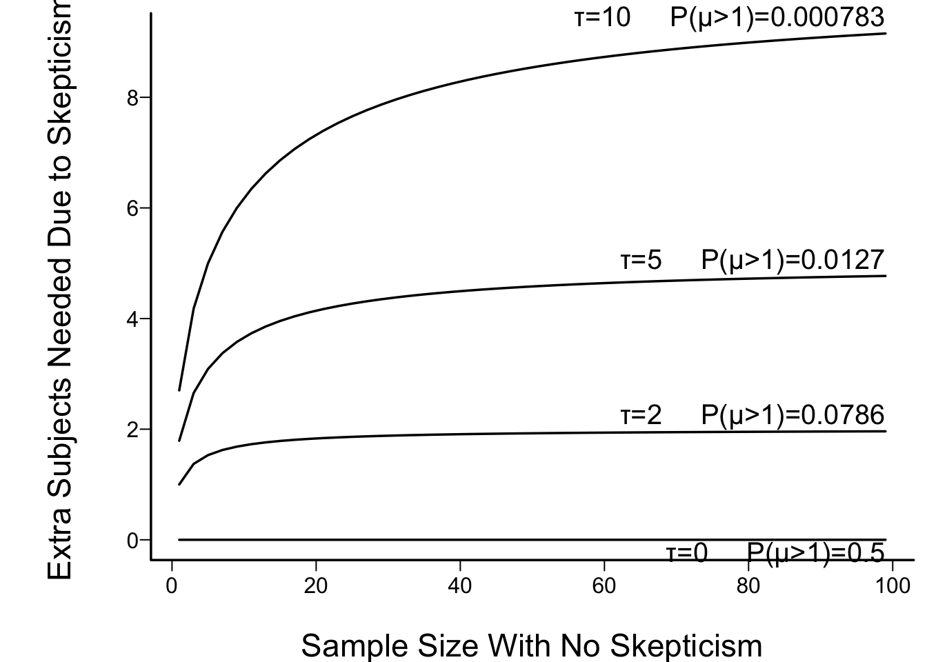
* Increase in sample size needed to overcome skepticism: $n - m$
* In figure below the prior prob($\mu > 1$) is also shown. This is $1 - \Phi(\sqrt{\tau})$
```{r skepn}
#| fig.cap: "Effect of discounting by a skeptical prior with mean zero and precision τ: the increase needed in the sample size in order to achieve the same posterior probability of μ > 0 as with the flat (non-informative) prior. τ=10 corresponds to a very skeptical prior, giving almost no chance to a large μ (μ > 1)."
spar(bty='l')
z <- list()
n <- seq(1, 100, by=2)
for(tau in c(0, 2, 5, 10))
  z[[paste0('τ=', tau, '     P(μ>1)=',
            format(1 - pnorm(sqrt(tau)), digits=3, scientific=1))]] <-
    list(x=n, y=0.5 * (n + sqrt(n^2 + 4 * n * tau)) - n)

labcurve(z, pl=TRUE, xlab='Sample Size With No Skepticism',
         ylab='Extra Subjects Needed Due to Skepticism', adj=1)
```
* Optimistic prior: effectively <b>adds</b> observations
## Contrasting Frequentist and Bayesian Evidence and Errors
* Let E=true unknown efficacy measure
+ what is generating the difference in effects in the data
+ difference in true means, log odds ratio, log hazard ratio, etc.
+ E=0: no treatment effect
+ E>0: benefit of new treatment
* Frequentist:
+ attempt to show data implausible if E=0
+ no probability statement about E; E is either 0 or nonzero
* Bayesian:
+ probability statement about E using posterior ("current") probs
+ E almost always thought of as continuous (P(E=0) = 0)
+ P(E > c \| data)
+ c=0: get evidence for <i>any</i> efficacy
+ c>0: get evidence for efficacy > some amount
+ There are no "errors"
+ Errors can only be made by decision makers when actions constrained to all-or-nothing
### Frequentist vs Bayes: Study Design
#### Frequentist
* Design study to have α=0.05 β=0.1
* Once data available, these no longer relevant since they apply to sequences of other trials, not this trial
* α depends on intentions, β on a single value of E
* Can also design for precision: solve for n such that 0.95 CL expected to have width w
#### Bayesian
* Choose prior for E allowing for uncertainty in true effect
* Design study to have prob ≥ 0.9 of achieving P(E > c) > 0.95 or to achieve credible interval width w
### Type of Errors
* Need to be careful about the use of the term 'error', as α is **not** the probability of making an error
* α is a conditional probability of making an _assertion_ of an effect **when any such assertion is by definition wrong**
* It is a trigger/alarm probability
* α is conditional on H<sub>0</sub> and ignores all data
#### Frequentist
* Type I assertion probability α: P(declare efficacy when E=0) = P(test stat > threshold when E=0)
* Type II assertion probability: P(fail to declare efficacy when E=c for some particular arbitrary c)
* α never drops no matter how large is n
#### Bayesian {-}
* P(E > c \| data)
* If act as if efficacious, P(error) is 1 - PP
* If act as if ineffective, P(error) is PP
### Example: p=0.03
#### Frequentist
* Conclude efficacy
* This is either right or wrong; no prob associated with true unknown E
* Exact interpretation: if E=0 and one ran an infinite sequence of identical trials, one would see an observed E ≥ that observed 0.03 of the time
#### Bayesian
* PP is its own error probability
### Example: p=0.2
#### Frequentist
* Can't conlude E=0 but fail to have evidence for E≠0
* No measure for P(E=0) available
#### Bayesian
* Simple PP of no effect or harm: P(E < 0)
### Clinical Significance
#### Frequentist
* With large n, trivial effect can yield p < 0.05
#### Bayesian
* Compute PP that true effect more than trivial
### p=0.04, 5 other trials "negative"
#### Frequentist
* No way to take the other 5 trials into account other that using non-quantitative subjective arguments
#### Bayesian
* Skepticism about efficacy for current trial already captured in the prior
* Or other trials could be used to form a prior, or Bayesian hierarchical model
## Problems Caused by Use of Arbitrary Thresholds
* Thresholding in general is arbitrary and detrimental to asessing totality of evidence
+ true for both frequentist and Bayesian
* Leads to false confidence
+ once known that evidence measure below or above threshold, stakeholders act as if no uncertainty (@goo99tow, @alt95abs, @gre96eff)
* Example honest sentence that is harder to take out of context:<br>Treatment B probably (0.94) resulted in lower BP and was probably (0.78) safer than treatment A
## Example: Is a Randomization Faulty? {#sec-evidence-rand}
Consider an example that demonstrates the stark contrast between frequentist and Bayesian inference. Here is the setup:
* An RCT's simple randomization algorithm appears to be producing an imbalance in an intended 1:1 randomization
* The number of persons assigned to treatments A and B is currently nA=130 and nB=94
* Is the randomization algorithm assigning persons to treatment A with probability $\theta = \frac{1}{2}$?
<!-- as of 2024-11-06 was 152 vs 108
as of 2025-01-27 157 vs 117
as of 2025-01-28 158 vs 119 -->
### Frequentist Approach
* Does not use any prior information about $\theta$
* Form a null hypothesis $\theta = \frac{1}{2}$
* Compute a p-value to gauge the compatibility of the data with the null hypothesis
* p = probability of getting data as or more extreme than 130:94 in either direction (2-tailed p)
* It is a measure of how surprising the data are under $H_0$
* Also compute a confidence interval for $\theta$
```{r}
nA <- 130
nB <- 94
# nA <- 152
# nB <- 108
bt <- binom.test(nA, nA + nB, p=0.5)
bt
pval <- bt$p.value
p3   <- round(pval, 3)
# Compute more accurate Wilson compatibility interval
binconf(nA, nA + nB)
```
* The results cast doubt on the assumption that $\theta = \frac{1}{2}$ since the compatibility of the data with $\theta = \frac{1}{2}$ is only `r p3`
* **But** many investigators misinterpret p-values as providing the probability of getting results as extreme as those observed if $H_0$ is true
+ This is **not** what p provides
+ It is the probability of getting results as **or more** extreme
+ So we can't say that we would obtain results as extreme as ours `r p3` of the time if the randomization algorithm is working perfectly
+ I.e., we can't say that we have just witnessed an event that only occurs `r p3` of the time when the probability of being allocated to treatment A is $\frac{1}{2}$, because p is not the probability of the event we've witnessed
+ The probability of getting results as extreme as ours in either direction is given by the calculation below
```{r}
pas <- 2 * dbinom(nA, nA + nB, 0.5)
pas
```
* The proportion of the p-value that comes from more extreme data than those observed rather than "as extreme" is `r 1 - round(pas / pval, 2)`
+ $\rightarrow$ we can't say exactly that the p-value gauges the compatibility of **our data** with $H_0$
* The probability of observing any one dataset is low (and is zero when the response variable is continuous)
+ It is not even very likely to observe data that are most concordant with $H_0$ (equal frequencies allocated to A and B) when $H_0$ is true
+ This probability is:
```{r}
dbinom(round((nA + nB)/2), nA + nB, 0.5)
```
* What is the evidence $\theta \neq \frac{1}{2}$?
* p=`r round(pval, 3)` is only very indirectly related to this, since it is not a probability about $\theta$ and because p applies **only if** $\theta=\frac{1}{2}$ (also there is the "more extreme" vs. "as extreme" issue)
* More importantly what is the evidence that the randomization ratio is non-trivially different from 1:1?
### Likelihoodist Approach
* Since p-values are effectively probabilities of "someone else's data" under $H_0$ and do not represent the likelihood of observing **our** data, there are better measures of evidence against $H_0$ [See [this](https://mzloteanu.substack.com/p/a-secret-third-way-likelihoodist) for an excellent tutorial on likelihoodist statistics by Mircea Zloteanu]{.aside}
* These are Bayesian measures (see below) and the likelihood ratio (LR) used in the likelihoodist school of inference
* Here the LR is the ratio of probability of getting the **observed** data without assuming $H_0$ and the probability assuming $H_0$
* The higher the LR the more evidence against $H_0$, with values greater than 10 typically taken to mean [strong evidence](https://www.sciencedirect.com/science/article/pii/S0895435621001323)
* LR computed below uses the _maximum_ likelihood without assuming $H_0$ in comparison with the likelihood assuming $H_0$
```{r}
theta_mle  <- nA / (nA + nB)    # maximum likelihood estimate of theta
LR <- dbinom(nA, nA + nB, theta_mle) / dbinom(nA, nA + nB, 0.5)
LR <- round(LR, 2)
LR
```
* This indicates strong evidence against the assertion that $\theta = \frac{1}{2}$ because the probability of observing the data that were observed for nA and nB without assuming $H_0$ is `r LR` $\times$ the probability of observing the **same** data assuming $H_0$
### Bayesian Approach
* Bayes is about uncovering the hidden data generating mechanism
* Use the data and prior information to try to uncover $\theta$
* We **do** have prior information about $\theta$: the probability of assigning a person to treatment A is very unlikely to be outside $[0.4, 0.6]$ or someone would have noticed the algorithm's defect much earlier
* Choose a prior for $\theta$ such that $\Pr(\theta < 0.4) = \Pr(\theta > 0.6) = 0.05$
* We want to bring evidence that the true unknown $\theta$ is non-trivially different from $\frac{1}{2}$
* So compute $\Pr(|\theta - \frac{1}{2}| > 0.02)$
* Beta distribution is convenient to use for the prior for $\theta$
* Beta distribution has parameters $\alpha, \beta$
* Assumine the prior is symmetric around $\frac{1}{2} \rightarrow \alpha = \beta$
* Solve for $\alpha$ such that $\Pr(\theta < 0.4) = 0.05$:
```{r}
g <- function(a) pbeta(0.4, a, a) - 0.05
alpha <- round(uniroot(g, c(1, 5000))$root, 2)
beta  <- alpha
alpha
```
* Prior is beta(`r alpha`, `r alpha`)
* The data distribution is binomial with parameters $\theta$ and $N = nA + nB$
* The posterior distribution is beta($\alpha + nA - 1, \beta + nB - 1$) (see [this](https://en.wikipedia.org/wiki/Beta_distribution#Bayesian_inference))
* Note this is a conditional probability given **our** data, not needing to consider data **more extreme** than ours
* Plot the prior and posterior distributions, and also plot the posterior distribution with a non-informative (NI) prior
```{r}
thetas <- seq(0, 1, length=200)
g <- function(type, p) data.frame(Type=type, theta=thetas, p=p)
d1 <- g('Prior',         p=dbeta(thetas, alpha, beta))
d2 <- g('Posterior',     p=dbeta(thetas, alpha + nA - 1, beta + nB - 1))
d3 <- g('Posterior, NI', p=dbeta(thetas, nA, nB))
d  <- rbind(d1, d2, d3)
ggplot(d, aes(x=theta, y=p, color=Type)) + geom_line() + xlab(expression(theta)) + ylab('')
```
The posterior mean for $\theta$ is $\frac{\alpha + nA - 1}{\alpha + \beta + N - 2}$ which is
```{r}
tmean <- round((alpha + nA - 1) / (alpha + beta + nA + nB - 2), 3)
tmean
```
as compared with the sample proportion of `r round(nA / (nA + nB), 3)`. Under the assumption that very large defects would have been detected earlier, the posterior mean is likely to be closer to $\theta$ than the sample proportion, which is more easily overinterpreted.
* The probability that the true unknown $\theta$ deviates from $\frac{1}{2}$ by more than 0.02 is
```{r}
p <- 1 - (pbeta(0.52, alpha + nA - 1, beta + nB -1) -
          pbeta(0.48, alpha + nA - 1, beta + nB -1))
p <- round(p, 3)
p
```
* Given our prior and the current randomization frequencies, the probability that the randomization algorithm is more than trivially defective is `r p`
* This has a more direct interpretation than the frequentist analysis, and accounts for clinical and not just statistical significance
* Because this is a Bayesian procedure there are no multiplicies from multiple looks, so the posterior probability of a non-trivial defect can be recalculated when more patients are randomized; p-values would need to be adjusted for multiplicies (and there is no unique way to do that)