20 Challenges of Analyzing High-Dimensional Data

Biomarker Uncertainty Principle:
A molecular signature can be either parsimonious or predictive, but not both.
— FE Harrell, 2009

We have more data than ever, more good data than ever, a lower proportion of data that are good, a lack of strategic thinking about what data are needed to answer questions of interest, sub-optimal analysis of data, and an occasional tendency to do research that should not be done.
— FE Harrell, 2015

20.1 Background

High-dimensional data are of at least three major types:

Data collected on hundreds of thousands or millions of subjects with a diverse array of variables
Time series of biologic signals collected every few milliseconds
Extremely large data arrays where almost all the variables are of one type (the main topic here)

The last data class includes such areas as

functional imaging
gene microarray
SNPs for genome-wide association studies
RNA seq
exome sequencing
mass spectrometry

The research yield of analysis of such data has been disappointing to date, for many reasons such as:

Biology is complex
Use of non-reproducible research methodology
Use of unproven statistical methods
Multiple comparison problems and double dipping¹
Failure to demonstrate value of information over and above the information provided by routine clinical variables, blood chemistry, and other standard medical tests
Inadequate sample size for the complexity of the analytic task
Overstatement of results due to searching for “winning” markers without understanding bias, regression to the mean (Section 14.8), and overfitting

¹ Double dipping refers to using the same data to test a hypothesis that was formulated from a confession from the tortured dataset.

Regarding double dipping/multiplicity a beautiful example is the dead salmon fMRI study by Bennett et al. in which the standard method of analyzing fMRI data by voxels was shown to find brain activation regions even in the dead brain (see prefrontal.org/files/posters/Bennett-Salmon-2009.pdf).

Wired, 2009-09-18.

Unfortunately, a large number of papers in genomics and imaging research have pretended that feature selection has no randomness, and have validated predictions in the same dataset used to find the signals, without informing the bootstrap or cross-validation procedure about the data mining used to derive the model so that the resampling procedure could repeat all feature selection steps afresh for each resample (Ambroise & McLachlan (2002)). Only by re-running all data analysis steps that utilized \(Y\) for each resample can an unbiased estimate of future model performance be obtained.

20.2 Global Analytic Approaches

Let \(X_{1}, X_{2}, \ldots, X_{p}\) denote an array of candidate features (gene expressions, SNPs, brain activation, etc.) and \(Y\) the response, diagnosis, or patient outcome being predicted.

20.2.1 One-at-a-Time Feature Screening

OaaT feature screening involves choosing a measure of association such as Pearson’s \(\chi^2\) statistic², computing all \(p\) association measures against \(Y\), and choosing those \(X\) features whose association measure exceeds a threshold. This is by far the most popular approach to feature discovery (and often to prediction, unfortunately) in genomics and functional imaging. It is demonstrably the worst approach in terms of the reliability of the “winning” and “losing” feature selection and because it results in poor predictive ability. The problems are due to multiple comparison problems, bias, typically high false negative rates, and to the fact that most features “travel in packs”, i.e., act in networks rather than individually. As if OaaT could not get any worse, many practitioners create “risk scores” by simply adding together individual regression coefficients computed from individual “winning” \(X\) features without regard to the correlation structure of the \(X\)s. This gives far too much weight to the selected \(X\)s that are co-linear with each other.

² Oddly, many practitioners of OaaT choose the more conservative and much slower to compute Fisher’s exact test.

There is a false belief that preventing a high false discovery rate solves the problems of OaaT. Most researchers fail to consider, among other things, the high false negative rate caused by their design and sample size.

OaaT results in highly overestimated effect sizes for winners, due to double dipping.

Multiplicity Corrections

In the belief that false positive discoveries are less desirable than missed discoveries, researchers employ multiplicity corrections to \(P\)-values arising from testing a large number of associations with \(Y\). The most conservative approach uses the addition or Bonferroni inequality to control the family-wise error risk which is the probability of getting any false positive association when the global null hypothesis that there are no true associations with \(Y\) holds. This can be carried out by testing the \(p\) associations against \(\frac{\alpha}{p}\) where \(\alpha=0.05\) for example. A less conservative approach uses the false discovery rate (FDR), better labeled the false discovery risk or false discovery probability. Here one controls the fraction of false positive associations. For example one sets the critical value for association statistics to a less severe threshold than dictated by Bonferroni’s inequality, by allowing \(\frac{1}{10}^{\mathrm th}\) of the claimed associations (those with the smallest \(P\)-values) to be false positives.

It is an irony that the attempt to control for multiplicity has led not only to missed discoveries and abandonment of whole research areas but has resulted in increased bias in the “discovered” features’ effect estimates. When using stepwise regression, the bias in regression coeffients comes not from multiplicity problems arising when experimentwise \(\alpha=0.05\) is used throughout but from using an \(\alpha\) cutoff \(< \frac{1}{2}\) for selecting variables. By selecting variables on the basis of small \(P\)-values, many of the selected variables were selected because their effects were overestimated, then regression to the mean sets in.

Concentrating on false discovery probabilities and ignoring false non-discovery probabilities is a mistake. Confidence in selecting “winners” and “losers” should come for example from narrow confidence intervals for ranks of feature importance as discussed below.

20.2.2 Forward Stepwise Variable Selection

Forward stepwise variable selection that does an initial screening of all the features, adds the most significant one, then attempts to add the next most significant feature, after adjusting for the first one, and so on. This approach is unreliable. It is only better than OaaT in two ways: (1) a feature that did not meet the threshold for the association with \(Y\) without adjusting for other features may become stronger after the selection of other features at earlier steps, and (2) the resulting risk score accounts for co-linearities of selected features. On the downside, co-linearities make feature selection almost randomly choose features from correlated sets of \(X\)s, and tiny changes in the dataset will result in different selected features.

20.2.3 Ranking and Selection

Feature discovery is really a ranking and selection problem. But ranking and selection methods are almost never used. An example bootstrap analysis on simulated data is presented later. This involves sampling with replacement from the combined \((X, Y)\) dataset and recomputing for each bootstrap repetition the \(p\) association measures for the \(p\) candidate \(X\)s. The \(p\) association measures are ranked. The ranking of each feature across bootstrap resamples is tracked, and a 0.95 confidence interval for the rank is derived by computing the 0.025 and 0.975 quantiles of the estimated ranks.

This approach puts OaaT in an honest context that fully admits the true difficulty of the task, including the high cost of the false negative rate (low power). Suppose that features are ranked so that a low ranking means weak estimated association and a high ranking means strong association. If one were to consider features to have “passed the screen” if their lower 0.95 confidence limit for their rank exceeds a threshold, and only dismisses features from further consideration if the upper confidence limit for their rank falls below a threshold, there would correctly be a large middle ground where features are not declared either winners or losers, and the researcher would be able to only make conclusions that are supported by the data. Readers of the classic Absence of Evidence paper Altman & Bland (1995) will recognize that this ranking approach solves the problem.

An example of bootstrap confidence intervals where multivariable modeling was used rather than OaaT association measures is in the course notes for Regression Modeling Strategies, Section 5.4. An example where the bootstrap is used in the context of OaaT is below.

20.2.4 Joint modeling of All Features Simultaneously using Shrinkage

This approach uses multivariable regression models along with penalized maximum likelihood estimation, random effects / hierarchical modeling, or skeptical Bayesian prior distributions for adjusted effects of all \(p\) \(X\) features simultaneously. Feature effects (e.g., log odds ratios) are discounted so as to prevent overfitting/over-interpretation and to allow these effects to be trusted out of context. The result is a high-dimensional regression model that is likely to provide well-calibrated absolute risk estimates and near-optimum predictive ability. Some of the penalization methods used are

lasso: a penalty on the absolute value of regression coefficient that highly favors zero as an estimate. This results in a large number of estimated coefficients being exactly zero, i.e., results in feature selection. The resulting parsimony may be illusory: bootstrap repetition may expose the list of “selected” features to be highly unstable.
ridge regression (penalty function that is quadratic in the regression coefficients): does not result in a parsimoneous model but is likely to have the highest predictive value
elastic net: a combination of lasso and quadratic penalty that has some parsimony but has better predictive ability than the lasso. The difficulty is simultaneously choosing two penalty parameters (one for absolute value of \(\beta\)s, one for their sum of squares).

20.2.5 Random Forest

This is an approach that solves some of the incredible instability and low predictive power of individual regression trees. The basic idea of random forest is that one fits a regression tree using recursive partitioning (CART) on multiple random samples of candidate features. Multiple trees are combined. The result is no longer a tree; it is an uninterpretable black box. But in a way it automatically incorporates shrinkage and is often competitive with other methods in predictive discriminantion. However random forests typically have unacceptable absolute predictive accuracy as reflected by calibration curves that are far from the line of identity, due to overfitting.

There is evidence that minimal-assumption methods such as random forests are “data hungry”, requiring as many as 200 events per candidate variable for their apparent predictive discrimination to not decline when evaluated in a new sample van der Ploeg et al. (2014).

20.2.6 Data Reduction Followed by Traditional Regression Modeling

This approach uses techniques such as principle component analysis (PCA) whereby a large number of candidate \(X\)s are reduced to a few summary scores. PCA is based on additively combining features so as to maximize the variation of the whole set of features that is explained by the summary score. A small number of PCA scores are then put into an ordinary regression model (e.g., binary logistic model) to predict \(Y\). The result is sometimes satisfactory though no easier to interpret than shrinkage methods.

20.2.7 Model Approximation

Also called pre-conditioning, this method is general-purpose and promising (Paul et al. (2008),Shen et al. (2004),Ambler et al. (2002)). One takes a well-performing black box (e.g., random forest or full penalized regression with \(p\) features) that generates predicted responses \(\hat{Y}\) and incorporates the right amount of shrinkage to make the predictions well-calibrated. Then try to find a smaller set of \(X\)s that can represent \(\hat{Y}\) with high accuracy (e.g., \(R^{2} \geq 0.9\)). Forward stepwise variable selection may be used for this purpose^[Here one is developing a mechanistic prediction where the true \(R^{2}\) is 1.0.}. This sub-model is an approximation to the “gold-standard” full black box. The ability to find a well-performing approximation is a test of whether the predictive signal is parsimoneous. If one requires 500 \(X\)s to achieve an \(R^{2} \geq 0.9\) in predicting the gold-standard predictions \(\hat{Y}\), then it is not possible to be parsimoneous and predictive.

A major advantage of model approximation is that if the original complex model was well calibrated by using appropriate shrinkage, the smaller approximate model inherits that shrinkage.

20.2.8 Incorporating Biology into High-Dimensional Regression Models

This approach is likely to result in the most trustworthy discoveries as well as the best predictive accuracy, if existing biological knowledge is adequate for specification of model structure. This is a structured shrinkage method where pathway (e.g., gene pathway) information is inserted directly in the model. One may encode multiple paths into a simultaneous regression model such that genes are “connected” to other genes in the same pathway. This allows an entire path to be emphasized or de-emphasized.

20.3 Simulated Examples

Monte Carlo simulation, when done in a realistic fashion, has the great advantage that one knows the truth, i.e., the true model and values of model parameters from which the artificial population was simulated. Then any derived model or estimates can be compared to the known truth. Also with simulation, one can easily change the sample size being simulated so that the effect of sample size can be studied and an adequate sample size that leads to reliable results can be computed. One can also easily change the dimensionality of the features.

20.3.1 Simulation To Understand Needed Sample Sizes

One of the most common association measures used in genomic studies is the odds ratio. As shown in Section 6.8 and Figure 6.1 , the odds ratio (OR) is very difficult to estimate when the outcome is rare or when a binary predictive feature has a prevalence far from \(\frac{1}{2}\). That is for the case when only a single pre-specified is estimated. When screening multiple features for interesting associations, one is effectively estimating a large number of ORs, and in order to make correct decisions about which features are promising and which aren’t, one must be able to control the margins of error of the entire set of OR estimates.

In the following simulation consider varying sample size \(n\) and number of candidate features \(p\). We simulate \(p\) binary features with known true ORs against the diagnosis or outcome \(Y\). The true unknown ORs are assumed to have a normal\((\mu=0,\sigma=0.25)\) distribution. We want to judge the ability to jointly estimate \(p\) associations and to rank order features by observed associations. The analysis that is simulated does not examine multiple \(X\)s simultaneously, so we save time by simulating just the total numbers of zeros and ones for each \(X\), given \(Y\).

Code

# For a vector of n binary outcomes y, simulates p binary features
# x that have a p-vector of fixed prevalences | y=0 of prev and are connected
# to y by a p-vector of true population odds ratios ors.
# Estimates the p odds ratios against the simulated outcomes and
# returns a data frame summarizing the information
#
# Note: the odds ratio for x predicting y is the same as the odds ratio
# for y predicting x.  y is simulated first so that all features will
# be analyzed against the same outcomes

sim <- function(y, prev, or) {
  n <- length(y)
  p <- length(prev)
  if(p != length(or)) stop('prev and or must have the same length')

  # prev = Pr(x=1 | y=0); let the odds for this be oprev = prev / (1-prev)
  # or = odds(x=1 | y=1) / oprev
  # Pr(x=1 | y=1) = oprev / ((1 / or) + oprev)

  oprev <- prev / (1 - prev)
  p1 <- oprev / ((1 / or) + oprev)
  n0 <- sum(y == 0)
  n1 <- sum(y == 1)
  # For n0 observations sample x so that Pr(x=0 | y=0) = prev
  nxy0 <- rbinom(p, size=n0, prob=prev)
  nxy1 <- rbinom(p, size=n1, prob=p1)

  # Compute p sample odds ratios
  sor <- (n0 - nxy0) * nxy1 / (nxy0 * (n1 - nxy1))
  g <- function(x) ifelse(x >= 1, x, 1 / x)
  r1 <- rank(sor)[which.max(or) ] / p
  r2 <- rank(or) [which.max(sor)] / p
  h <- function(u, lab) { u <- factor(u); levels(u) <- paste0(lab, ':', levels(u)); u}
  data.frame(prev, or, nx=nxy0 / n0, obsprev0=(nxy0 + nxy1) / n,
             obsprev=nxy1 / (nxy0 + nxy1), obsor=sor, n=n,
             N       =h(n, 'n'),
             Features=h(p, 'Features'),
             mmoe    =quantile(g(sor / or), 0.90, na.rm=TRUE),
             obsranktrue=r1, truerankobs=r2,
             rho=cor(sor, or, method='spearman', use='pair'))
}

Code

U <- NULL
set.seed(1)
for(n in c(50, 100, 250, 500, 1000, 2000)) {
  for(p in c(10, 50, 500, 1000, 2000)) {
    for(yprev in c(.1, .3)) {
      y <- rbinom(n, 1, yprev)
      prev <- runif(p, .05, .5)
      or <- exp(rnorm(p, 0, .25))
      u <- cbind(sim(y, prev, or),
                 Yprev=paste('Prevalence of Outcome', yprev, sep=':'))
      U <- rbind(U, u)
    }
  }
}
with(U, tapply(obsprev, Yprev, mean, na.rm=TRUE))

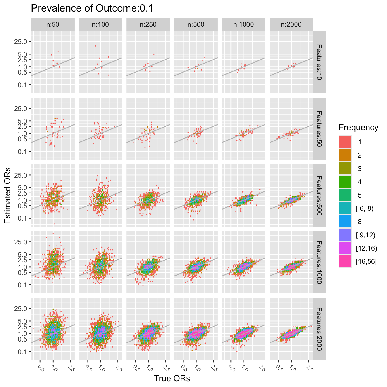
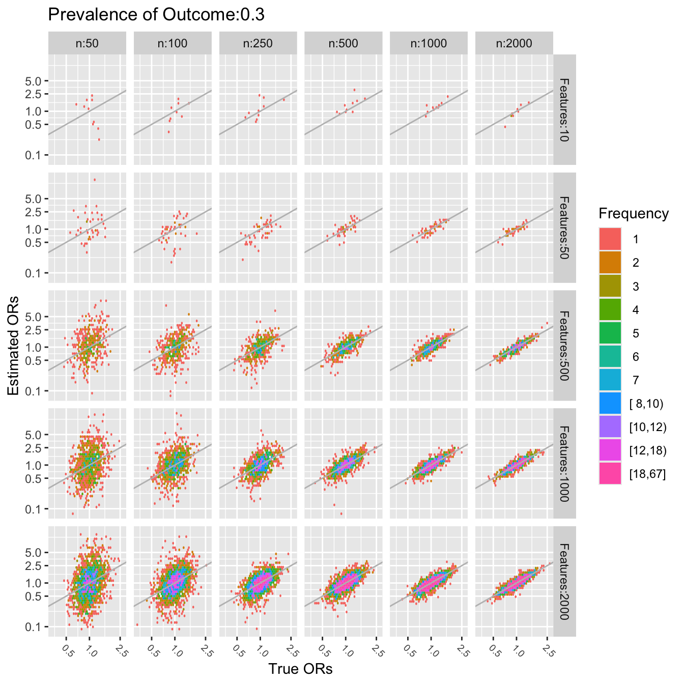
Prevalence of Outcome:0.1 Prevalence of Outcome:0.3 
                0.1007949                 0.3076869

In the plots below gray lines show the line of identity.

Code

require(ggplot2)
pl <- function(yprev) {
  br <- c(.01, .1, .5, 1, 2.5, 5, 25, 100)
  ggplot(subset(U, Yprev==paste0('Prevalence of Outcome:', yprev)),
         aes(x=or, y=obsor)) +
         stat_binhex(aes(fill=cut2(..count.., g=25)), bins=40) +
         facet_grid(Features ~ N) +
         ggtitle(paste('Prevalence of Outcome', yprev, sep=':')) +
         xlab('True ORs') + ylab('Estimated ORs') +
         scale_x_log10(breaks=br) + scale_y_log10(breaks=br) +
         guides(fill=guide_legend(title='Frequency')) +
         theme(axis.text.x = element_text(size = rel(0.8), angle=-45,
                                    hjust=0, vjust=1)) +
         geom_abline(col='gray')
}
pl(0.1)

Code

pl(0.3)

The last two figures use a log scale for the \(y\)-axis (estimated odds ratios), so the errors in estimating the odds ratios are quite severe. For a sample size of \(n=50\) one cannot even estimate a single pre-specified odds ratio. To be able to accurately assess 10 ORs (10 candidate features) requires about \(n=1000\). To assess 2000 features, a sample size of \(n=2000\) seems adequate only for the very smallest and very largest true ORs.

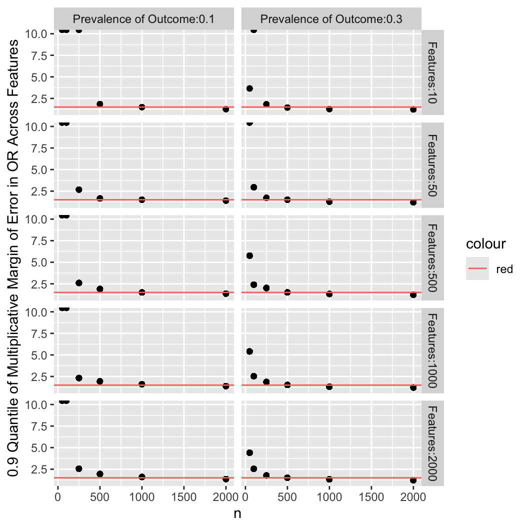
The plot below summarizes the previous plots by computing the 0.9 quantile of the multiplicative margin of error (fold change) over the whole set of estimated odds ratios, ignoring direction.

Code

ggplot(U, aes(x=n, y=mmoe)) + geom_point() + facet_grid(Features ~ Yprev) +
  geom_hline(aes(yintercept=1.5, col='red')) +
  ylim(1, 10) +
  ylab('0.9 Quantile of Multiplicative Margin of Error in OR Across Features')

Horizontal red lines depict a multiplicative margin of error (MMOE) of 1.5 which may be considered the minimally acceptable error in estimating odds ratios. This was largely achieved with \(n=1000\) for a low-incidence \(Y\), and \(n=500\) for a moderate-incidence \(Y\).

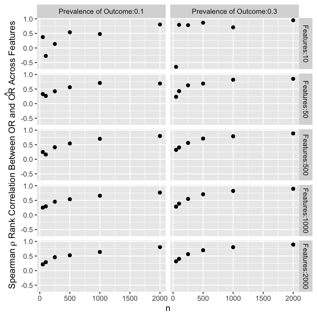
Another way to summarize the results is to compute the Spearman rank correlation between estimated and true underlying odds ratios over the entire set of estimates.

Code

ggplot(U, aes(x=n, y=rho)) + geom_point() +
  facet_grid(Features ~ Yprev) +
  ylab(expression(paste('Spearman ', rho, ' Rank Correlation Between ',
                        OR, ' and ', hat(OR), ' Across Features')))

One may desire a correlation with the truth of say 0.8 and can solve for the needed sample size.

20.3.2 Bootstrap Analysis for One Simulated Dataset

Suppose that one wanted to test \(p\) candidate features and select the most “significant” one for a validation study. How likely is the apparently “best” one to be truly the best? What is a confidence interval for the rank of this “winner”? How much bias in the OR does the selection process create? The bootstrap can be used to answer all of these questions without needing to assume anything about true population parameter values. The bootstrap can take into account many sources of uncertainty. We use the bootstrap to estimate the bias in the apparent highest and apparent lowest odds ratios—the two “winners”. The sample size of the simulated data is 600 subjects and there are 300 candidate features.

The bootstrap is based on sampling with replacement from the rows of the entire data matrix \((X, Y)\). In order to sample from the rows we need to generate raw data, not just numbers of “successes” and “failures” as in the last simulation.

Code

# Function to simulate the raw data
# prev is the vector of prevalences of x when y=0 as before
# yprev is the overall prevalence of y
# n is the sample size
# or is the vector of true odds ratios
sim <- function(n, yprev, prev, or) {
  y <- rbinom(n, 1, yprev)
  p <- length(prev)
  if(p != length(or)) stop('prev and or must have the same length')

  # prev = Pr(x=1 | y=0); let the odds for this be oprev = prev / (1-prev)
  # or = odds(x=1 | y=1) / oprev
  # Pr(x=1 | y=1) = oprev / ((1 / or) + oprev)

  oprev <- prev / (1 - prev)
  p1 <- oprev / ((1 / or) + oprev)
  x <- matrix(NA, nrow=n, ncol=p)
  for(j in 1 : p)
    x[, j] <- ifelse(y == 1, rbinom(n, 1, prob = p1[j]  ),
                             rbinom(n, 1, prob = prev[j]))
  list(x=x, y=y)
}

# Function to compute the sample odds ratios given x matrix and y vector
ors <- function(x, y) {
  p <- ncol(x)
  or <- numeric(p)
  for(j in 1 : p) {
    f <- table(x[, j], y)
    or[j] <- f[2, 2] * f[1, 1] / (f[1, 2] * f[2, 1])
  }
  or
}

Code

# Generate sample of size 600 with 300 features
# Log odds ratios have a normal distribution with mean 0 SD 0.3
# x have a random prevalence uniform [0.05, 0.5]
# y has prevalence 0.3

set.seed(188)
n <- 600; p <- 300
prev <- runif(p, .05, .5)
or   <- exp(rnorm(p, 0, .3))
z    <- sim(n, 0.3, prev, or)

# Compute estimated ORs
x <- z$x;   y <- z$y
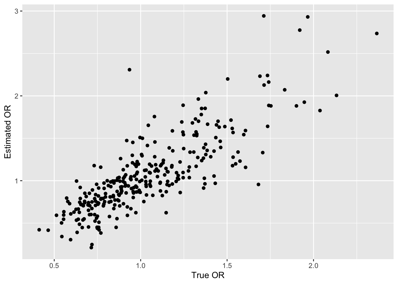
sor <- ors(x, y)
# Show how estimates related to true ORs
ggplot(data.frame(or, sor), aes(x=or, y=sor)) + geom_point() +
  xlab('True OR') + ylab('Estimated OR')

Code

# Print the largest estimated OR and its column number,
# and corresponding true OR, and similarly for the smallest.
largest   <- max(sor)
imax      <- which.max(sor)
true.imax <- or[imax]
mmoe.imax <- largest / true.imax
smallest  <- min(sor)
imin      <- which.min(sor)
true.imin <- or[imin]
mmoe.imin <- smallest / true.imin
cat('\nLargest observed OR\n')


Largest observed OR

Code

cat('OR:', round(largest, 2), '  Feature #', imax, '  True OR:',
    round(true.imax, 2), '  MMOE:', round(mmoe.imax, 2), '\n')

OR: 2.94   Feature # 90   True OR: 1.71   MMOE: 1.72

Code

cat('Rank of winning feature among true ORs:', sum(or <= or[imax]), '\n\n')

Rank of winning feature among true ORs: 285

Code

cat('Smallest observed OR\n')

Smallest observed OR

Code

cat('OR:', round(smallest, 2), '  Feature #', imin, '  True OR:',
    round(true.imin, 2), '  MMOE:', round(mmoe.imin, 2), '\n')

OR: 0.21   Feature # 99   True OR: 0.71   MMOE: 0.3

Next use the bootstrap to get an estimate of the MMOE for the observed largest OR, and a 0.95 confidence interval for the true unknown rank of the largest observed OR from among all the features. 1000 bootstrap resamples are drawn. In estimating the MMOE we are estimating bias in the largest log odds ratio when a new “largest” OR is found in each bootstrap resample. That estimated OR is compared to the OR evaluated in the whole sample for the same column number. This is also done for the “smallest” OR.

Code

set.seed(11)
B <- 1000
ranksS <- ranksL <- mmoeS <- mmoeL <- numeric(B)

for(k in 1 : B) {
  # Draw a sample of size n with replacement
  i <- sample(1 : n, n, replace=TRUE)
  # Compute sample ORs on the new sample
  bor      <- ors(x[i, ], y[i])
  blargest <- max(bor)
  bmax     <- which.max(bor)
  ranksL[k] <- sum(bor <= largest)
  mmoeL[k]  <- blargest / sor[bmax]
  bsmallest <- min(bor)
  bmin      <- which.min(bor)
  ranksS[k] <- sum(bor <= smallest)
  mmoeS[k]  <- bsmallest / sor[bmin]
}

The bootstrap geometric mean MMOE for the smallest odds ratio was zero due to small frequencies in some \(X\)s. The median bootstrap MMOE was used to bias-correct the observed smallest OR, while the geometric mean was used for the largest.

Code

pr <- function(which, ranks, mmoe, mmoe.true, estor, or.true) {
  gm <- exp(mean(log(mmoe)))
  cat(which, 'OR\n')
  cat('CL for rank:', quantile(ranks, c(0.025, 0.975)),
      '  Median MMOE:', round(median(mmoe), 2),
      '  Geometric mean MMOE:', round(gm, 2),
      '\nTrue MMOE:', round(mmoe.true, 2), '\n')
  bmmoe <- if(which == 'Largest') gm else median(mmoe)
  cat('Bootstrap bias-corrected', tolower(which), 'OR:',
      round(estor / bmmoe, 2),
      '  Original OR:', round(estor, 2),
      '  True OR:', round(or.true, 2),
      '\n\n')
}
pr('Largest',  ranksL, mmoeL, mmoe.imax, largest,  true.imax)

Largest OR
CL for rank: 294 299   Median MMOE: 1.45   Geometric mean MMOE: 1.52 
True MMOE: 1.72 
Bootstrap bias-corrected largest OR: 1.93   Original OR: 2.94   True OR: 1.71

Code

pr('Smallest', ranksS, mmoeS, mmoe.imin, smallest, true.imin)

Smallest OR
CL for rank: 0 5   Median MMOE: 0.34   Geometric mean MMOE: 0 
True MMOE: 0.3 
Bootstrap bias-corrected smallest OR: 0.62   Original OR: 0.21   True OR: 0.71

The bootstrap bias-corrected ORs took the observed extreme ORs and multiplied them by their respective bootstrap geometric mean or median MMOEs. The bias-corrected estimates are closer to the true ORs.

The data are consistent with the observed smallest OR truly being in the bottom 5 and the observed largest OR truly being in the top 7.

Here is some example wording that could be used in a statistical analysis plan: We did not evaluate the probability that non-selected genes are truly unimportant but will accompany the planned gene screening results with a bootstrap analysis to compute 0.95 confidence intervals for the rank of each gene, using a non-directional measure of association when ranking. The “winning” genes will have high ranks in competing with each other (by definition) but if the lower confidence limits include mid- to low-level ranks the uncertainty of these winners will be noted. Conversely, if the upper confidence intervals of ranks of “losers” extend well into the ranks of “winners”, the uncertainty associated with our ability to rule out “losers” for further investigation will be noted.

20.3.3 Sample Size to Estimate a Correlation Matrix

An abstraction of many of the tasks involved in both unsupervised learning (observation clustering, variable clustering, latent trait analysis, principal components, etc.) and supervised learning (statistical regression models or machine learning to predict outcomes) is the estimation of a correlation matrix involving potential predictors and outcomes. Even with linear regression where one is interested in estimating \(p\) regression coefficients \(\beta\) plus an intercept, one must deal with collinearities in order to estimate \(\beta\) well. This involves inverting the matrix of all sums of squares and cross-products of the predictors, so again it is akin to estimating a large correlation matrix.

Section 8.5.2 showed how to estimate the sample size needed to estimate a single linear or Spearman correlation coefficient \(r\) to within a given margin of error. A simple summary of what is in that section is that \(n=300\) is required to estimate \(r\) to within a margin of error of \(\pm 0.1\) with 0.95 confidence. Consider now the estimation of an entire correlation matrix involving \(p\) continuous variables, which gives rise to \(\frac{p(p-1)}{2}\) distinct \(r\) values to estimate.

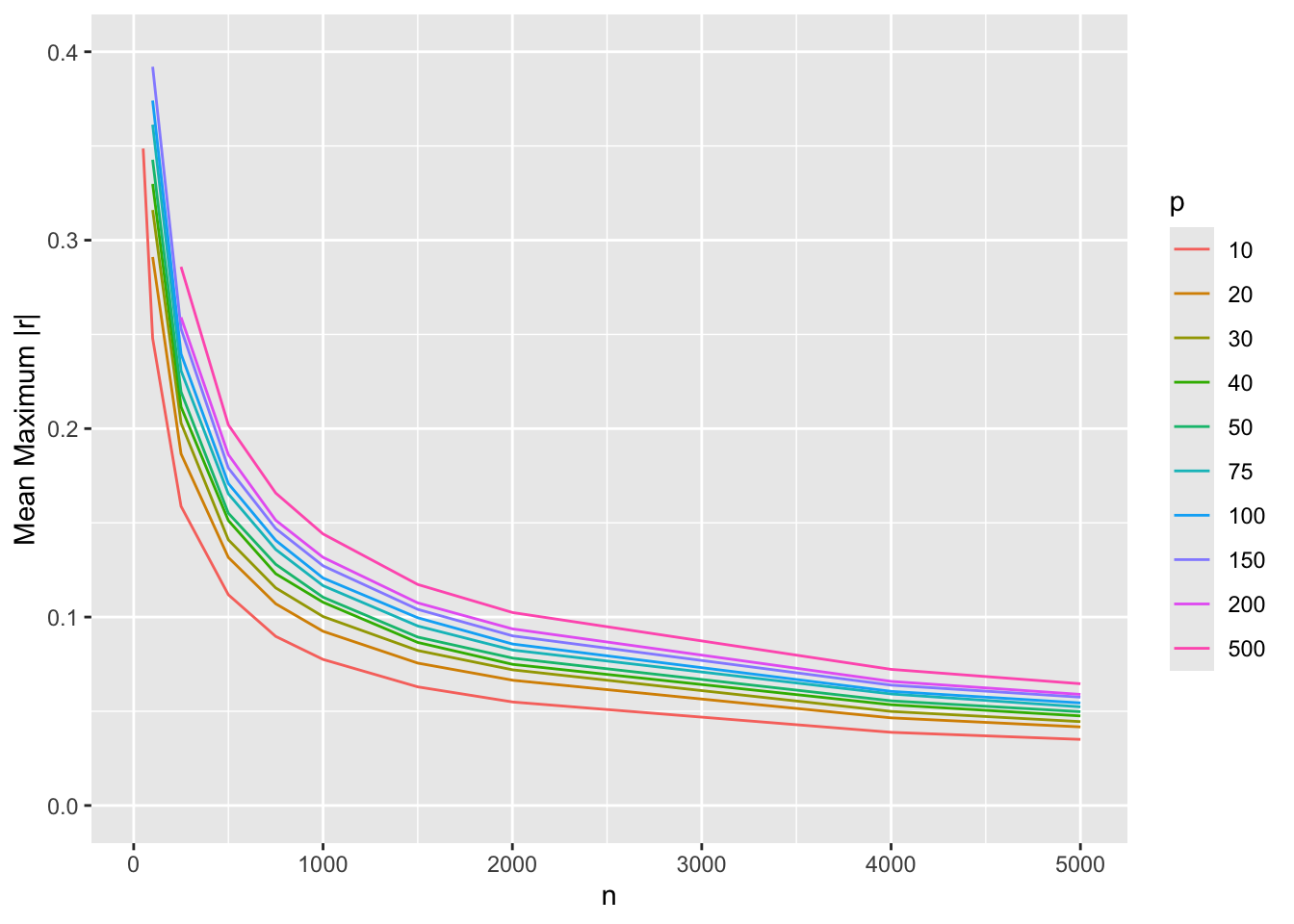
True correlation coefficients close to zero are the most difficult to estimate (have the lowest precision of the estimated \(r\)s), so consider the situation in which all \(p\) variables are uncorrelated. Every \(r\) value should be zero, but random chance leads to very erroneously large coefficient estimates for small \(n\). Quantify the estimation error for an entire matrix by considering the maximum absolute \(r\) over the \(\frac{p(p-1)}{2}\) pairs of variables. Simulate data from normal distributions for given \(n\) and \(p\), drawing 250 random samples for each \(n, p\) combination. Compute the mean of the maximum absolute correlation coefficients over the 250 simulations. The results are shown below.

See this for the simulation code.

Code

w <- readRDS('rflow-simcorr.rds')
ggplot(w, aes(x=n, y=r, col=factor(p))) + geom_line() +
       ylim(0, 0.4) +
       guides(color=guide_legend(title='p')) +
       ylab('Mean Maximum |r|')

Figure 20.1: Average over 250 simulations of \(\frac{p(p-1)}{2}\) maximum absolute correlation coefficients for various sample sizes \(n\) and number of variables \(p\)

The bottom curve is for \(p=10\) variables, i.e., for estimating all 45 \(r\)s among them. The minimum acceptable sample size \(n\) may be taken as about \(n=700\) as this leads to a maximum correlation estimation error of 0.1. The error is cut in half for \(n=2000\). The top curve, for \(p=500\) variables, leads to selection of \(n=2000\) as a minimum sample size for sufficiently accurate estimation of the entire correlation matrix, with \(n=4000\) improving precision further by about \(\frac{1}{4}\). For most studies, \(p=500\) may be thought of as the largest unstructured (e.g., not informed by biological pathways) problem that can be reliably studied. For a sample size of \(n=500\) it may be unreliable to study more than 10 variables in free-form.

20.3.4 One-at-a-Time Bootstrap Feature Selection

When there is a large number of candidate features it is computationally difficult to fit penalized models containing all features simultaneously. We may resort to assessing the predictive value of each feature on its own, adjusted for a fixed set of covariates. Bootstrapping this process to get confidence intervals on importance ranks of all candidate features is easy. In the following example we simulate a binary response variable that is partially predicted by age, and we include each of 400 binary features in a model with age. The features are assumed to have log odds ratios following a Gaussian distribution with mean zero and standard deviation 0.25. The importance measure we’ll use is the gold standard model likelihood ratio \(\chi^2\) statistic with 2 d.f. It does not matter that this statistic counts the age effect, as we will be comparing all the 2 d.f. statistics with different features in the model but with age always present.

First simulate the data, with a sample size of 500. Put the features into a \(500\times 400\) matrix. The simulated data use a model with all effects included simultaneously even though we won’t analyze the data this way. Features are assumed to be independent and to have prevalence 0.5.

Code

require(rms)
n <- 500   # number of subjects
p <- 400   # number of candidate features
B <- 300   # number of bootstrap repetitions
set.seed(9)
age   <- rnorm(n, 50, 8)  # Gaussian distribution for age
betas <- rnorm(p, 0, 0.15)
X     <- matrix(rbinom(n * p, 1, 0.5), nrow=n)
xb    <- 0.07 * (age - 50) + (X - 0.5) %*% betas
y     <- rbinom(n, 1, plogis(xb))
# Function to compute ranks of 2 d.f. LR chi-square over p features
r <- function(s = 1 : n, pl=FALSE) {
  chisq <- numeric(p)
  for(j in 1 : p) {
    d <- data.frame(age, y, x=X[,j])[s, ]
    f <- lrm(y ~ age + x, data=d)
    chisq[j] <- f$stats['Model L.R.']
  }
  if(pl) hist(chisq, nclass=30, xlab='2 d.f. Chi-squares', main='')
  rank(chisq)
}
# Using the original sample, plot the chi-square ranks against true betas
orig.ranks <- r(pl=TRUE)

Code

plot(betas, orig.ranks, xlab=expression(beta), ylab='Rank')

The last plot is a sign of how difficult it is to select winners from among 400 competing features when the sample size is not huge. There is no apparent relationship between model strength and true feature regression coefficients.

Now bootstrap the process 300 times to get bootstrap nonparametric percentile confidence intervals for ranks.

Code

set.seed(11)
g <- function() {
  R <- matrix(NA, nrow=B, ncol=p)
  for(i in 1 : B) R[i, ] <- r(sample(n, replace=TRUE))
  R
}
R <- runifChanged(g)  # run time 6m

Compute 400 0.95 confidence intervals for ranks.

Code

ci <- apply(R, 2, quantile, c(0.025, 0.975))
winner <- which.max(orig.ranks)

Plotting these 400 confidence intervals fully reveals the difficulty of the task. But for our purposes it suffices to show the confidence interval for the apparent winning feature, which is feature number 280. Let’s first compute the age-adjusted \(\chi^2\) for this feature.

Code

x <- X[, winner]
f <- lrm(y ~ age + x, x=TRUE, y=TRUE)
anova(f, test='LR')

Likelihood Ratio Statistics for `y`
	χ²	d.f.	P
age	16.02	1	<0.0001
x	11.26	1	0.0008
TOTAL	25.73	2	<0.0001

The p-value for this feature would not survive a Bonferroni adjustment for 400 comparisons. The bootstrap confidence interval for the importance rank of the feature is

Code

ci[, winner]

   2.5%   97.5% 
216.975 400.000

The winner was replicated as the winner in at least 2.5% of the bootstrap resamples, but the lower confidence interval shows that the data are consistent with the winner almost being in the lower half of the 400 features’ importance.