```{r setup, include=FALSE}
require(Hmisc)
require(qreport)
hookaddcap() # make knitr call a function at the end of each chunk
# to try to automatically add to list of figure
options(prType='html')
getRs('qbookfun.r')
knitr::set_alias(w = 'fig.width', h = 'fig.height',
cap = 'fig.cap', scap ='fig.scap')
```
# Comparing Two Proportions
`r mrg(bmovie(8), ddisc(8))`
## Overview
* Compare dichotomous independent variable with a dichotomous outcome
+ Independent variables: Exposed/Not, Treatment/Control, Knockout/Wild Type, etc.
+ Outcome (dependent) variables: Diseased/Not or any Yes/No outcome
* Continuous outcomes often dichotomized for analysis (bad idea)
+ Consider $t$-tests (Chapter 5) or Non-parametric methods (Chapter 7)
## Normal-Approximation Test
* Two independent samples
| | Sample 1 | Sample 2 |
|-----|-----|-----|
| Sample size | $n_1$ | $n_2$ |
| Population probability of event | $p_1$ | $p_2$ |
| Sample probability of event | $\hat{p}_1$ | $\hat{p}_2$ |
* Null Hypothesis, $H_{0}: p_{1}=p_{2}=p$
* Estimating the variance
+ Variance of $\hat{p}_{i} = p_{i}(1-p_{i})/n_{i}$ for $i = 1, 2$
+ Variance of $\left(\hat{p}_1 - \hat{p}_2\right)$ is the sum of the variances, which under $H_{0}$ is
$$
p(1-p)[\frac{1}{n_{1}}+\frac{1}{n_{2}}]
$$
+ We estimate this variance by plugging $\hat{p}$ into $p$, where
$$
\hat{p} = \frac{n_{1}\hat{p}_{1}+n_{2}\hat{p}_{2}}{n_{1}+n_{2}}
$$
is the pooled estimate of the probability under $H_{0}: p_1 = p_2 = p$
* Test statistic which has approximately a normal distribution under $H_{0}$ if $n_{i}\hat{p}_{i}$ are each large enough:
$$
z = \frac{\hat{p}_{1} -
\hat{p}_{2}}{\sqrt{\hat{p}(1-\hat{p})[\frac{1}{n_{1}}+\frac{1}{n_{2}}]}}
$$
* To test $H_{0}$ we see how likely it is to obtain a $z$ value as far or farther out in the tails of the normal distribution than $z$ is
* We don't recommend using the continuity correction
* Example: <br> Test whether the population of women whose age at first birth $\leq 29$ has the same probability of breast cancer as women whose age at first birth was $\geq 30$. This dichotomization is highly arbitrary and we should really be testing for an association between age and cancer incidence, treating age as a continuous variable.
* Case-control study (independent and dependent variables interchanged); $p_{1}=$ probability of age at first birth $\geq 30$,
etc.
| | with Cancer | without Cancer |
|-----|-----|-----|
| Total # of subjects | $3220~~(n_1)$ | $10245~~(n_2)$ |
| # age $\geq 30$ | $683$ | $1498$ |
| Sample probabilities | $0.212~~(\hat{p}_1$) | $0.146~~(\hat{p}_2$) |
| Pooled probability | $\frac{683 + 1498}{3220 + 10245} = 0.162$ | |
<!-- $$\begin{array}{c}--->
<!-- n_{1}=3220, n_{2}=10245, \\--->
<!-- \hat{p}_{1}=\frac{683}{3220}=0.212, \\--->
<!-- \hat{p}_{2}=\frac{1498}{10245} = 0.146 \\--->
<!-- \hat{p}=\frac{683+1498}{3220+10245} = 0.162 \\--->
* Estimate the variance
+ $\mathrm{variance}(\hat{p}_{1}-\hat{p}_{2}) = \hat{p}(1-\hat{p})\times \left[\frac{1}{n_{1}}+\frac{1}{n_{2}}\right] = 5.54 \times 10^{-5}$
+ $SE = \sqrt{\mathrm{variance}} = 0.00744$
* Test statistic
+ $z = \frac{0.212-0.146}{0.00744} = 8.85$
* 2-tailed $P$-value is $< 10^{-4}$
```{r ptwo}
n1 <- 3220;     n2 <- 10245
p1 <- 683 / n1; p2 <- 1498 / n2
pp <- (n1 * p1 + n2 * p2) / (n1 + n2)
se <- sqrt(pp * (1 - pp) * (1 / n1 + 1 / n2))
z  <- (p1 - p2) / se
pval <- 2 * (1 - pnorm(abs(z)))
round(c(p1=p1, p2=p2, pooled=pp, se=se, z=z, pval=pval), 4)
```
* We do not use a $t$-distribution because there is no $\sigma$ to estimate (and hence no "denominator d.f." to subtract)
## $\chi^2$ Test
* If $z$ has a normal distribution, $z^2$ has a $\chi^2$ distribution with 1 d.f. (are testing a single difference against zero)
* The data we just tested can be shown as a $2\times 2$ contingency table
| | Cancer + | Cancer - |
|-----|-----:|-----:|
| Age $\leq 29$ | 2537 | 8747 | 11284 |
| Age $\geq 30$ | 683 | 1498 | 2181 |
| | 3220 | 10245 | 13465 |
* In general, the $\chi^2$ test statistic is given by
$$\sum_{ij} \frac{(\mathrm{Obs}_{ij}-\mathrm{Exp}_{ij})^2}{\mathrm{Exp}_{ij}}$$
* $\mathrm{Obs}_{ij}$ is the observed cell frequency for row $i$ column $j$
* $\mathrm{Exp}_{ij}$ is the expected cell frequency for row $i$ column $j$
+ Expected cell frequencies calculating assuming $H_0$ is true
+ $\mathrm{Exp}_{ij} = \frac{\mathrm{row }~i~\mathrm{ total} \times \mathrm{column}~j~\mathrm{total}}{\mathrm{grand total}}$
+ e.g. $\mathrm{Exp}_{11} = \frac{11284 \times 3220}{13465} = 2698.4$
* For $2 \times 2$ tables, if the observed cell frequencies are labeled
| $a$ | $b$ |
|-----|-----|
| $c$ | $d$ |
the $\chi^{2}$ test statistic simplifies to
$$
\frac{N[ad - bc]^{2}}{(a+c)(b+d)(a+b)(c+d)},
$$
where $N=a+b+c+d$. Here we get $\chi^{2}_{1} = 78.37 = z^{2}$ from above.
```{r pearsonchi}
x <- matrix(c(2537, 8747, 683, 1498), nrow=2, byrow=TRUE)
x
chisq.test(x, correct=FALSE)
# Also compute more accurate P-value based on 1M Monte-Carlo simulations
chisq.test(x, correct=FALSE, simulate.p.value=TRUE, B=1e6)
```
* Don't need Yates' continuity correction
<!-- Eq. 10.5--->
* Note that even though we are doing a 2-tailed test we use only the right tail of the $\chi^{2}_{1}$ distribution; that's because we have squared the difference when computing the statistic, so the sign is lost.
* This is the ordinary Pearson $\chi^2$ test
## Fisher's Exact Test
* Is a misnomer in the sense that it computes probabilities exactly, with no normal approximation, but only after changing what is being tested to condition on the number of events and non-events
* Because frequencies are discrete and because of the conditioning, the test is conservative ($P$-values too large)
* Is exact only in the sense that actual type I error probability will not **exceed** the nominal level
* The ordinary Pearson $\chi^2$ works fine (even when an expected cell frequency is as low as 1.0, contrary to popular belief)
* We don't use Yates' continuity correction because it was developed to make the normal approximation test yield $P$-values that are more similar to Fisher's test, i.e., to be more conservative
* The attempt to obtain exact unconditional $P$-values for the simple $2\times 2$ contingency table has stumped frequentist statisticians for many decades @cho15elu
* By contrast, Bayesian posterior probabilities for the true unconditional quantity of interest are exact
+ Frequentist confidence limits and $P$-values are approximate because they use the sample space, and the sample space is discrete when the response variable is categorical
+ Bayes does not consider the sample space, only the parameter space, which is almost always continuous
* See [stats.stackexchange.com/questions/14226](https://stats.stackexchange.com/questions/14226) for discussion
## Sample Size and Power for Comparing Two Independent Samples
* Power $\uparrow$ as
+ $n_{1}, n_{2} \uparrow$
+ $\frac{n_{2}}{n_{1}} \rightarrow 1.0$ (usually)
+ $\Delta = |p_{1}-p_{2}| \uparrow$
+ $\alpha \uparrow$
* There are approximate formulas such as the recommended methods in Altman based on transforming $\hat{p}$ to make it have a variance that is almost independent of $p$
* Example: Using current therapy, 0.5 of the population is free of infection at 24 hours. Adding a new drug to the standard of care is expected to increase the percentage infection-free to 0.7. If we randomly sample 100 subjects to receive standard care and 100 subjects to receive the new therapy, what is the probability that we will be able to detect a certain difference between the two therapies at the end of the study?
$$
p_{1}=.5, p_{2}=.7, n_{1}=n_{2}=100
$$
results in a power of 0.83 when $\alpha=0.05$
```{r bpower}
require(Hmisc)
bpower(.5, .7, n1=100, n2=100)
```
* When computing sample size to achieve a given power, the sample size $\downarrow$ when
+ power $\downarrow$
+ $\frac{n_{2}}{n_{1}} \rightarrow 1.0$
+ $\Delta \uparrow$
+ $\alpha \uparrow$
* Required sample size is a function of both $p_{1}$ and $p_{2}$
* Example:
How many subjects are needed to detect a 0.8 fold decrease in the probability of colorectal cancer if the baseline probability of cancer is $0.0015$? Use a power of 0.8 and a type-I error probability of 0.05.
$$\begin{array}{c}
p_{1}=0.0015, p_{2}=0.8\times p_{1}=0.0012, \alpha=0.05, \beta=0.2 \\
n_{1}=n_{2}=235,147
\end{array}$$
(Rosner estimated 234,881)
```{r bsamsize}
bsamsize(.0015, 0.8 * .0015, alpha=0.05, power=0.8)
```
Formulas for power and sample size may be seen as `R` code found at<br>
[github.com/harrelfe/Hmisc/blob/master/R/bpower.s](https://github.com/harrelfe/Hmisc/blob/master/R/bpower.s).
## Confidence Interval
An approximate $1-\alpha$ 2-sided CL is given by
$$\hat{p}_{1}-\hat{p}_{2} \pm z_{1-\alpha/2} \times\sqrt{\frac{\hat{p}_{1}(1-\hat{p}_{1})}{n_{1}}+\frac{\hat{p}_{2}(1-\hat{p}_{2})}{n_{2}}}$$
where $z_{1-\alpha/2}$ is the critical value from the normal
distribution (1.96 when $\alpha=0.05$).
The CL for the number of patients needed to be treated to save one
event may simply be obtained by taking the reciprocal of the two
confidence limits.^[If a negative risk reduction is included in the confidence interval, set the NNT to $\infty$ for that limit instead of quoting a negative NNT. There is more to this; see [bit.ly/datamethods-nnt](http://bit.ly/datamethods-nnt).]
## Sample Size for a Given Precision
* Goal: Plan a study so that the margin of error is sufficiently small
* The margin of error ($\delta$) is defined to be half of the confidence interval width. For two proportions,
$$
\delta = z_{1-\alpha/2} \times\sqrt{\frac{\hat{p}_{1}(1-\hat{p}_{1})}{n_{1}}+\frac{\hat{p}_{2}(1-\hat{p}_{2})}{n_{2}}}
$$
* Basing the sample size calculations on the margin of error can lead to a study that gives _scientifically_ relevant results even if the results are not _statistically_ significant.
* Example: Suppose that the infection risk in a population is $0.5$ and a reduction to $0.4$ is believed to be a large enough reduction that it would lead to a change in procedures. A study of a new treatment is planned so that enough subjects will be enrolled for the margin of error is $0.05$. Consider these two possible outcomes:
1. The new treatment is observed to decrease infections by $0.06$ ($0.95$ CI: $[0.11, 0.01]$). The confidence interval does not contain $0$, so we have indirect evidence^[To obtain direct evidence requires Bayesian posterior probabilities.] that the new treatment is effective at reducing infections. $0.1$ is also within the confidence interval limits.
1. The new treatment is observed to decrease infections by only $0.04$ ($0.95$ CI: $[0.09, -0.01]$). The confidence interval now contains $0$, so we do not have enough evidence to reject the supposition that there is no effect of the treatment on reducing infections if we are bound to an arbitrary $\alpha=0.05$. However, the confidence interval also does not contain $0.10$, so we are able to indirectly rule out a _scientifically_ relevant decrease in infections.
* For fixed $n_{1} = n_2 = n$, confidence intervals for proportions have the maximum width, when $p_{1} = p_{2} = 0.5$. This can be shown by:
+ Recall that the variance formula for the difference in two proportions when calculating a confidence interval is
$$
\frac{p_{1}(1-p_{1})}{n_{1}}+\frac{p_{2}(1-p_{2})}{n_{2}}
$$
+ When $p_{1} = p_{2} = p$ and $n_{1} = n_2 = n$, the variance formula simplifies to
$$
\frac{p(1 - p)}{n}+\frac{p (1- p)}{n} = 2\frac{p(1 - p)}{n}
$$
+ Then, for any fixed value of $n$ ($e.g. n = 1$ or $10$), $2\frac{p(1 - p)}{n}$ is largest when $p = 0.5$. With $p= 0.5$, the variance formula further simplifies to
$$
2\frac{.25}{n} = \frac{1}{2n}
$$
* Using $\alpha = 0.05$ ($z_{1-\alpha/2} = 1.96$), the worst-case margin of error will be
$$
\delta = 1.96 \sqrt{\frac{1}{2n}}
$$
* By solving for $n$, we can rearrange this formula to be
$$
n = \frac{1.92}{\delta^2}
$$
* This formula then gives the number of subjects needed in each group $n$ to obtain a given margin of error $\delta$. For a margin of error of $0.05$ ($\delta = 0.05$), $n = \frac{1.92}{0.05^2} = 768$ subjects in each group.
```{r moeprop}
diff <- .05
qnorm(.975)^2 / 2 / (diff ^ 2)
```
<!-- In the case $n_{1}=n_{2}=n, \alpha=0.05$, the confidence interval has maximum width with $p_{1}$ and $p_{2}$ are near 0.5. As a worse case the margin of error is then $1.96/\sqrt{2n}$. The $n$ required to achieve a margin of error of $\delta$ at the 0.95 confidence level is $1.92/\delta^{2}$. For example, to approximate the difference in the incidence probability of stroke between males and females to at worst $\pm 0.05$ at the 0.95 level would require 768 patients in each group.--->
## Relative Effect Measures{#sec-prop-rem}
* We have been dealing with risk differences which are measures of absolute effect
* Measures of relative effect include risk ratios and odds ratios
* Risk ratios are easier to interpret but only are useful over a limited range of prognosis (i.e., a risk factor that doubles your risk of lung cancer cannot apply to a subject having a risk above 0.5 without the risk factor)
* Odds ratios can apply to any subject
* In large clinical trials treatment effects on lowering probability of an event are often constant on the odds ratio scale
* OR = Odds ratio = $\frac{\frac{p_{1}}{1-p_{1}}}{\frac{p_{2}}{1-p_{2}}}$
* Testing $H_{0}$: OR=1 is equivalent to testing $H_{0}:p_{1}=p_{2}$
* There are formulas for computing confidence intervals for odds ratios
* Odds ratios are most variable when one or both of the probabilities are near 0 or 1
* We compute CLs for ORs by anti-logging CLs for the log OR
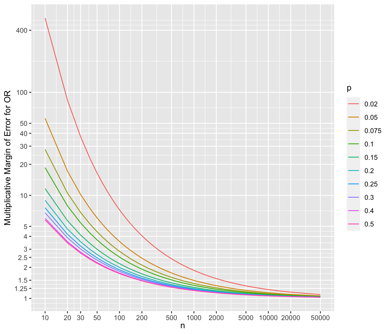
* In the case where $p_{1}=p_{2}=0.05$ and $n_{1}=n_{2}=n$, the standard error of the log odds ratio is approximately $\sqrt{\frac{42.1}{n}}$
* The common sample size $n$ needed to estimate the true OR to within a factor of 1.5 is 984 with $p$s in this range
* To show the multiplicative margins of error^[Value by which to multiply the observed odds ratio to obtain the upper 0.95 confidence limit or to divide the observed odds ratio to obtain the lower 0.95 limit. The confidence interval for a ratio should always be constructed on the log scale (unless using the excellent profile likelihood interval which is transformation-invariant). We compute the margin of error on the log ratio scale just as we do for means. The margin of error can be defined as $\frac{1}{2}$ of the width of the confidence interval for the log ratio. If you anti log that margin of error you get the multiplicative factor, i.e., the multiplicative margin of error. Suppose that the MMOE is 1.5. This means that you can get the 0.95 confidence interval for the ratio by taking the ratio’s point estimate and dividing it by 1.5 and then multiplying it by 1.5. You can loosely say that our point estimate can easily be off by a factor of 1.5.] for a range of sample sizes and values of $p$. For each scenario, the margin of error assumes that both unknown probability estimates equal $p$.
```{r mmeor,w=7,h=6,cap='Multiplicative margin of error related to 0.95 confidence limits of an odds ratio, for varying $n$ and $p$ (different curves), assuming the unknown true probability in each group is no lower than $p$',scap='Multiplicative margin of error for odds ratios'}
#| label: fig-prop-mmeor
require(ggplot2)
d <- expand.grid(n=c(seq(10, 1000, by=10), seq(1100, 50000, by=100)),
                 p=c(.02, .05, .075, .1, .15, .2, .25, .3, .4, .5))
d$selor <- with(d, sqrt(2 / (p * (1 - p) * n)))
d$mmoe  <- with(d, exp(qnorm(0.975) * selor))
mb <- c(1, 1.25, 1.5, 2, 2.5, 3, 4, 5, 10, 20, 30, 40, 50, 100, 400)
ggplot(aes(x=n, y=mmoe, color=factor(p)), data=d) +
  geom_line() +
  scale_x_log10(breaks=c(10,20,30,50,100,200,500,1000,2000,5000,10000,
                  20000,50000)) +
  scale_y_log10(breaks=mb, labels=as.character(mb)) +
  xlab(expression(n)) + ylab('Multiplicative Margin of Error for OR') +
  guides(color=guide_legend(title=expression(p)))
```
## Comprehensive example
### Study Description
* Consider patients who will undergo coronary artery bypass graft surgery (CABG)
* Mortality risk associated with open heart surgery
* Study question: Do emergency cases have a surgical mortality that is different from that of non-emergency cases?
* Population probabilities
+ $p_1$: Probability of death in patients with emergency priority
+ $p_2$: Probability of death in patients with non-emergency priority
* Statistical hypotheses
+ $H_0: p_1 = p_2$ (or $\mathrm{OR} = 1$)
+ $H_1: p_1 \neq p_2$ (or $\mathrm{OR} \neq 1$)
### Power and Sample Size
* Prior research shows that just over $0.1$ of surgeries end in death
* Researchers want to be able to detect a 3 fold increase in risk
* For every 1 emergency priority, expect to see 10 non-emergency
* $p_1 = 0.3$, $p_2 = 0.1$, $\alpha = 0.05$, and power} = 0.90
* Calculate sample sizes using the PS software for these values and other combinations of $p_1$ and $p_2$
| $(p_1, p_2)$ |**(0.3, 0.1)**|(0.4, 0.2)|(0.03, 0.01)|(0.7, 0.9) |
|-----|-----:|-----:|-----:|-----:|
| $n_1$ |**40**|56|589|40 |
| $n_2$ |**400**|560|5890|400 |
Check PS calculations against the `R` `Hmisc` package's
`bsamsize` function.
```{r surgss}
round(bsamsize(.3, .1, fraction=1/11, power=.9))
round(bsamsize(.4, .2, fraction=1/11, power=.9))
round(bsamsize(.7, .9, fraction=1/11, power=.9))
```
### Collected Data
In-hospital mortality figures for emergency surgery and other surgery
| Surgical Priority| Dead| Alive |
|-----|-----:|-----:|
| Emergency|6| 19 |
| Other|11|100 |
* $\hat{p}_1 = \frac{6}{25} = 0.24$
* $\hat{p}_2 = \frac{11}{111} = 0.10$
### Statistical Test
```{r surgdata}
n1 <- 25;     n2 <- 111
p1 <- 6 / n1; p2 <- 11 / n2
or <- p1 / (1 - p1) / (p2 / (1 - p2))
or
# Standard error of log odds ratio:
selor <- sqrt(1 / (n1 * p1 * (1 - p1)) + 1 / (n2 * p2 * (1 - p2)))
# Get 0.95 confidence limits
cls <- exp(log(or) + c(-1, 1) * qnorm(0.975) * selor)
cls
tcls <- paste0(round(or, 2), ' (0.95 CI: [', round(cls[1], 2),
               ', ', round(cls[2], 2), '])')
# Multiplying a constant by the vector -1, 1 does +/-
x <- matrix(c(6, 19, 11, 100), nrow=2, byrow=TRUE)
x
chisq.test(x, correct=FALSE)
```
<!-- Ignore the warning about the $\chi^2$ approximation.--->
* Interpretation
+ Compare odds of death in the emergency group $\left(\frac{\hat{p}_1}{1-\hat{p}_1}\right)$ to odds of death in non-emergency group $\left(\frac{\hat{p}_2}{1-\hat{p}_2}\right)$
+ Emergency cases have `r tcls` fold increased odds of death during surgery compared to non-emergency cases.
#### Fisher's Exact Test
Observed marginal totals from emergency surgery dataset <br>
| \multicolumn{1}{l}{} | \multicolumn{1}{c}{Dead} | \multicolumn{1}{l}{Alive} \cline{2-3} |
|-----|-----|-----|
| Emergency | $a$ | $b$ | $25$ \cline{2-3} |
| Other | $c$ | $d$ | $111$ \cline{2-3} |
| \multicolumn{1}{l}{} | \multicolumn{1}{c}{$17$} | \multicolumn{1}{c}{$119$} | \multicolumn{1}{c}{$136$} |
* With fixed marginal totals, there are 18 possible tables ($a = 0, 1, \ldots 17$)
* Can calculated probability of each of these tables
+ $p$-value: Probability of observing data as extreme or more extreme than we collected in this experiment
* Exact test: $p$-value can be calculated "exactly" (not using the $\chi^2$ distribution to approximate the $p$-value)
<br>
```{r fet}
fisher.test(x)
```
Note that the odds ratio from Fisher's test is a conditional maximum
likelihood estimate, which differs from the unconditional maximum
likelihood estimate we obtained earlier.
* Fisher's test more conservative than Pearson's $\chi^2$ test (larger $P$-value)
## Logistic Regression for Comparing Proportions
`r mrg(bmovie(9), ddisc(9))`
* When comparing $\geq 2$ groups on the probability that a categorical outcome variable will have a certain value observed (e.g., $P(Y=1)$), one can use the Pearson $\chi^2$ test for a contingency table (or the less powerful Fisher's "exact" test)
* Such analyses can also be done with a variety of regression models
* It is necessary to use a regression model when one desires to analyze more than the grouping variable, e.g.
+ analyze effects of two grouping variables
+ adjust for covariates
* For full generality, the regression model needs to have no restrictions on the regression coefficients
+ Probabilities are restricted to be in the interval $[0,1]$ so an additive risk model cannot fit over a broad risk range
+ Odds ($\frac{p}{1-p}$) are restricted to be in $[0, \infty]$
+ Log odds have no restrictions since they can be in $[-\infty, \infty]$
* So log odds is a good basis for regression analysis of categorical $Y$
+ default assumption of additivity of effects needs no restrictions
+ will still translate to probabilities in $[0,1]$
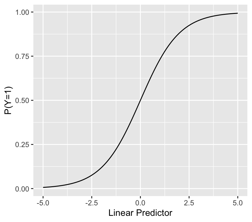
* The binary logistic regression model is a model to estimate the probability of an event as a flexible function of covariates
* Let the outcome variable $Y$ have the values $Y=0$ (non-event) or $Y=1$ (event)
$$\mathrm{Prob}(Y = 1 | X) = \frac{1}{1 + \exp(-(\beta_0 + \beta_1 x_1 + \beta_2 x_2 + \beta_3 x_3 + \ldots))}$$
* The sum inside the inner () is called the linear predictor (LP)
* The binary logistic model relates LP (with no restrictions) to the event probability as so:
```{r lrmshape}
#| label: fig-prop-logisticfun
#| fig-width: 4.25
#| fig-height: 3.75
#| fig-cap: "The logistic function"
lp <- seq(-5, 5, length=150)
ggplot(mapping=aes(lp, plogis(lp))) + geom_line() +
  xlab('Linear Predictor') + ylab('P(Y=1)')
```
* Notes about LP:
+ for a given problem the range may be much narrower than $[-4,4]$
+ when any predictor $X_j$ with a non-zero $\beta_j$ is categorical, LP cannot take on all possible values within its range, so the above plot will have gaps
* As a special case the model can estimate and compare two probabilities as done above, through an odds ratio
* Logistic regression seems like an overkill here, but it sets the stage for more complex frequentist analysis as well as Bayesian analysis
* For our case the model is as follows
* Consider groups A and B, A = reference group<br> $[x]$ denotes 1 if $x$ is true, 0 if $x$ is false<br> Define the expit function as the inverse of the logit function, or $\mathrm{expit}(x) = \frac{1}{1 + \exp(-x)}$
\begin{array}{ccc}
P(Y = 1 | \mathrm{group}) &=& \frac{1}{1 + \exp(-(\beta_0 + \beta_1 [\mathrm{group } B]))} \\
&=& \mathrm{expit}(\beta_0 + \beta_1 [\mathrm{group } B])\\
P(Y = 1 | \mathrm{group A}) &=& \mathrm{expit}(\beta_0)\\
P(Y = 1 | \mathrm{group B}) &=& \mathrm{expit}(\beta_0 + \beta_1)
\end{array}
$\beta_0 =$ log odds of probability of event in group A $= \log(\frac{p_1}{1 - p_1}) = \mathrm{logit}(p_1)$<br>
$\beta_1 =$ increase in log odds in going from group A to group B = <br> $\log(\frac{p_2}{1 - p_2}) - \log(\frac{p_1}{1 - p_1}) = \mathrm{logit}(p_2) - \mathrm{logit}(p_1)$<br>
$\exp(\beta_1) =$ group B : group A odds ratio $= \frac{\frac{p_2}{1 - p_2}}{\frac{p_1}{1 - p_1}}$ <br>
expit$(\beta_0) = p_1$ <br>
expit$(\beta_0 + \beta_1) = p_2$
* Once the $\beta$s are estimated, one quickly gets the B:A odds ratio and $\hat{p}_1$ and $\hat{p}_2$
* This model is **saturated**
+ has the maximum number of parameters needed to fully describe the situation (here, 2 since 2 groups)
+ saturated models **must** fit the data if the distributional and independence assumptions are met
+ logistic model has no distributional assumption
* Logistic regression is more general and flexible than the specialized tests for proportions
+ allows testing association on continuous characteristics
+ easily extends to more than two groups
+ allows adjustment for covariates
* Examples:<br>
+ assess effects of subjects' sex and country (Canada vs. US) on $P(Y=1)$ denoted by $p$<br> logit $p$ = constant + logit male effect + logit Canada effect
+ same but allow for interaction<br> logit $p$ = constant + logit male effect + logit Canada effect + special effect of being male if Canadian
+ latter model is saturated with 3 d.f. so fits as well as a model with 4 proportions
- unlike the overall Pearson $\chi^2$ test, allows testing interaction and
- separate effects of sex and country (e.g., 2 d.f. chunk test for whether there is a sex difference for either country, allowing for the sex effect to differ by country)
### Test Statistics
For frequentist logistic models there are 3 types of $\chi^2$ test statistics for testing the same hypothesis:
* likelihood ratio (LR) test (usually the most accurate) and is scale invariant^[The LR test statistic is the same whether testing for an absolute risk difference of 0.0, or for an odds or risk ratio of 1.0.]
+ Can obtain the likelihood ratio $\chi^2$ statistic from either the logistic model or from a logarithmic equation in the two proportions and sample sizes
* Score test (identical to Pearson test for overall model if model is saturated)
* Wald test (square of $\frac{\hat{\beta}}{\mathrm{s.e.}}$ in the one parameter case; misbehaves for extremely large effects)
* Wald test is the easiest to compute but $P$-values and confidence intervals from it are not as accurate. The score test is the way to exactly reproduce the Pearson $\chi^2$ statistic from the logistic model.
* As with $t$-test vs. a linear model, the special case tests are not needed once you use the logistic model framework
* Three usages of any of these test statistics:
+ individual test, e.g. sex effect in sex-country model without interaction
+ chunk test, e.g. sex + sex $\times$ country interaction 2 d.f. test<br>tests overall sex effect
+ global test of no association, e.g. 3 d.f. test for whether sex or country is associated with $Y$
### Frequentist Analysis Example
* Consider again our emergency surgery example
* String the observations out to get one row = one patient, binary $Y$
```{r lrmprop}
require(rms)
options(prType='html')
priority <- factor(c(rep('emergency', 25), rep('other', 111)), c('other', 'emergency'))
death <- c(rep(0, 19), rep(1, 6), rep(0, 100), rep(1, 11))
table(priority, death)
```
```{r lrmprop2}
d  <- data.frame(priority, death)
dd <- datadist(d); options(datadist='dd')
# rms package needs covariate summaries computed by datadist
f <- lrm(death ~ priority)
f
```
* Compare the LR $\chi^2$ of 3.2 with the earlier Pearson $\chi^2$ of 3.70
* The likelihood ratio (LR) $\chi^2$ test statistic and its $P$-value are usually a little more accurate than the other association tests
+ but $\chi^2$ distribution is still only an approximation to the true sampling distribution
* See that we can recover the simple proportions from the fitted logistic model:<br>
$\hat{p}_1 = \frac{11}{111} = 0.099 = \mathrm{expit}(-2.2073)$<br>
$\hat{p}_2 = \frac{6}{25} = 0.24 = \mathrm{expit}(-2.2073 + 1.0546)$
```{r lrmprop3}
summary(f)
```
* The point estimate and CLs for the odds ratio is the same as what we obtained earlier.
Add a random binary variable to the logistic model---one that is correlated with the surgical priority---to see the effect on the estimate of the priority effect
```{r lrmpropr}
set.seed(10)
randomUniform <- runif(length(priority))
random <- ifelse(priority == 'emergency', randomUniform < 1/3,
                                          randomUniform > 1/3) * 1
d$random <- random
table(priority, random)
```
```{r lrmpropr2}
lrm(death ~ priority + random)
```
The effect of emergency status is diminished, and the random grouping variable, created to have no relation to death in the population, has a large apparent effect.
### Bayesian Logistic Regression Analysis
* Has several advantages
+ All calculations are exact (to within simulation error) without changing the model
+ Can incorporate external information
+ Intuitive measures of evidence
+ Automatically handles zero-frequency cells (priors shrink probabilities a bit away from 0.0)
* Simple to use beta priors for each of the two probabilities
* But we'd need to incorporate a complex dependency in the two priors because we know more about how the two probabilities relate to each other than we know about each absolute risk
* Simpler to have a wide prior on $p_1$ and to have a non-flat prior on the log odds ratio
+ could back-solve and show dependency between knowledge of $p_1$ and $p_2$
* Use the same data model as above
* As before we use the `R` `brms` package which makes standard modeling easy
* Need two priors: for intercept $\beta_0$ and for log odds ratio $\beta_1$
* $\beta_0$: use a normal distribution that makes $p_1 = 0.05$ the most likely value (put mean at logit(0.05) = -2.944) and allows only a 0.1 chance that $p_1 > 0.2$; solve for SD $\sigma$ that accomplishes that
```{r normsolve}
# Given mu and value, solve for SD so that the tail area of the normal distribution beyond value is prob
normsolve <- function(mu, value, prob) (value - mu) / qnorm(1 - prob)
normsolve(qlogis(0.05), qlogis(0.2), 0.1)  # qlogis is R logit()
```
* We round $\sigma$ to 1.216
* For $\beta_1$ put a prior that has equal chance for OR $< 1$ as for OR $> 1$, i.e., mean for log OR of zero<br> Put a chance of only 0.1 that OR $> 3$
```{r normsolve2}
normsolve(0, log(3), 0.1)
```
* Round to 0.857
Compute the correlation between prior evidence for $p_1$ and $p_2$ by drawing 100,000 samples from the prior distributions. Also verify that prior probability $p_2 > p_1$ is $\frac{1}{2} =$ prob. OR $> 1$.
```{r priorcorr}
b0 <- rnorm(100000, qlogis(0.05), 1.216)
b1 <- rnorm(100000, 0, 0.857)
p1 <- plogis(b0)
p2 <- plogis(b0 + b1)
cor(b0, b1, method='spearman')
cor(p1, p2, method='spearman')
# Define functions for posterior probability operator and posterior mode
P <- mean   # proportion of posterior draws for which a condition holds
pmode <- function(x) {
  z <- density(x)
  z$x[which.max(z$y)]
  }

P(p2 > p1)
P(b1 > 0)
P(exp(b1) > 1)
```
To show that prior knowledge about $p_1$ and $p_2$ is uncorrelated when we don't know anything about the odds ratio, repeat the above calculation use a SD of 1000 for the log odds ratio:
```{r priorcorr2}
b1 <- rnorm(100000, 0, 1000)
p2 <- plogis(b0 + b1)
cor(p1, p2, method='spearman')
```
Now do Bayesian logistic regression analysis.
```{r bayesprop0}
require(brms)
# Tell brms/Stan to use all available CPU cores less 1 and to use
# cmdstan instead of rstan
options(mc.cores=parallel::detectCores() - 1, brms.backend='cmdstanr')
cmdstanr::set_cmdstan_path(cmdstan.loc)   # defined in ~/.Rprofile
```
```{r bayesprop}
p <- c(prior(normal(-2.944, 1.216), class='Intercept'),
       prior(normal(0, 0.857),      class='b'))
f <- brm(death ~ priority, data=d, prior=p, family='bernoulli', seed=123)
```
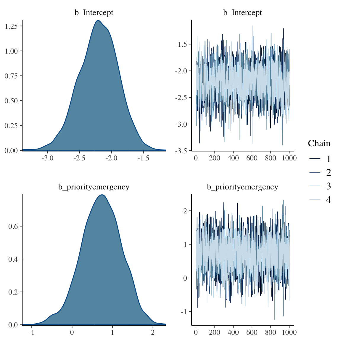
```{r bayesprop2,h=6,w=6}
f
plot(f)
```
```{r bayesprop3}
# Bring out posterior draws
w <- as.data.frame(f)
b0 <- w[, 'b_Intercept']
b1 <- w[, 'b_priorityemergency']
r  <- rbind(c(mean(b0), median(b0), pmode(b0)),
            c(mean(b1), median(b1), pmode(b1)),
            c(mean(exp(b1)), median(exp(b1)), pmode(exp(b1))))
colnames(r) <- c('Posterior Mean', 'Posterior Median', 'Posterior Mode')
rownames(r) <- c('b0', 'b1', 'OR')
round(r, 3)
```
Because the prior on the OR is conservative, the Bayesian posterior mode for the OR is smaller than the frequentist maximum likelihood estimate of 2.87.
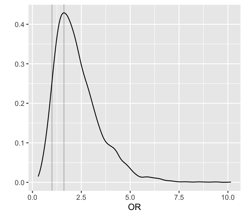
Below notice how easy it is to do Bayesian inference on derived quantities p1 and p2 which are functions of b0 and b1.
```{r bayesprop4}
#| label: fig-prop-bayesprop4
#| fig-height: 3.75
#| fig-width: 4.25
#| fig-cap: "Posterior distribution of odds ratio"
# 0.95 credible interval for log odds ratio and odds ratio
quantile(b1, c(0.025, 0.975))
quantile(exp(b1), c(.025, 0.975))
exp(quantile(b1, c(0.025, 0.975)))
# Posterior density of emergency:other odds ratio
ggplot(mapping=aes(x=exp(b1))) + geom_density() +
  xlab('OR') + ylab('') +
  geom_vline(xintercept=c(1, pmode(exp(b1))), alpha=I(0.25))
# Probability that OR > 1
P(exp(b1) > 1)
# Probability it is > 1.5
P(exp(b1) > 1.5)
# Probability that risk with emergency surgery exceeds that of
# non-emergency (same as P(OR > 1))
# plogis in R is 1/(1 + exp(-x))
P(plogis(b0 + b1) > plogis(b0))
# Prob. that risk with emergency surgery elevated by more than 0.03
P(plogis(b0 + b1) > plogis(b0) + 0.03)
```
Even though the priors for the intercept and log odds ratio are independent, the connection of these two parameters in the data likelihood makes the posteriors dependent as shown with Spearman correlations of the posterior draws below. Also get the correlation between evidence for the two probabilities. These have correlated priors even though they are unconnected in the likelihood function. Posteriors for $p_1$ and $p_2$ are less correlated than their priors.
```{r bayesprop2c}
cor(b0, b1, method='spearman')
cor(plogis(b0), plogis(b0 + b1), method='spearman')
```
To demonstrate the effect of a skeptical prior:
* Add random grouping to model as we did with the frequentist analysis
* Make use of prior information that this variable is unlikely to be important
* Put a prior on the log OR for this variable centered at zero with chance that the OR $> 1.25$ of only 0.05
```{r bayesprop5}
normsolve(0, log(1.25), 0.05)
p <- c(prior(normal(-2.944, 1.216), class='Intercept'),
       prior(normal(0, 0.857),      class='b', coef='priorityemergency'),
       prior(normal(0, 0.136),      class='b', coef='random'))

f2 <- brm(death ~ priority + random, data=d, prior=p, family='bernoulli',
          seed=121)
f2
```
* Effect of `random` is greatly discounted
* Posterior mean priority effect and its credible interval is virtually the same as the model that excluded `random`
James Rae and Nils Reimer have written a nice tutorial on using the `R` `brms` package for binary logistic regression available at
[bit.ly/brms-lrm](http://bit.ly/brms-lrm)
```{r echo=FALSE}
saveCap('06')
```