15 Analysis

flowchart LR
PA[Principled Analysis]
PA --> plan[Pre-specification to Limit Double Dipping]
PA --> rep[Reproducibility]
PA --> raw[Respect Raw Data in Analysis]
PA --> nd[Never Categorize Continuous or Ordinal Variables]
PA --> sc[Choose Statistics and Uncertainty Intervals Respecting the Design]
An[Analysis] --> Formal[Formal<br>See hbiostat.org/bbr] & DA[Descriptive]

Orders of Descriptive Analysis

flowchart TD
a1[First Order] --> b1[Summarize Distribution of X]
a2[Second Order] --> b2["Assess Shape and<br>Strength of Association<br>Between X and Y"]
a3[Third Order] --> b3["Assess How<br>Association Between<br>X and Y Varies with Z"]

Types of Descriptive Analysis

flowchart LR
HI[High Information Displays] --> AT[Avoid Tables<br>When X is Continuous]
HI --> NT[Nonparametric Smoothers]
HI --> Dist[Distributions Depicted With<br>Spike Histograms and<br>Extended Box Plots]
HI --> mov[General Approach:<br>Statistics in Moving<br>Overlapping Windows]
For[Formatting Analysis output]

R has thousands of packages for data analysis. A good way to explore these capabilities is to spend time with the CRAN Task Views.

15.1 Big Picture

For analysis the sky is the limit, but statistical principles should guide every step. Some of the general principles are

If there is to be a pivotal analysis there should be a statistical analysis plan (SAP) for this analysis that does not allow for many “statistician degrees of freedom.” The plan should be completed before doing any analysis that might inform analysis choices in a way that would bias the results (e.g., bias the estimate of treatment effect or bias standard errors of effects in a model).
All analyses should be completely reproducible. Explicitly state random number seeds if any random processes (bootstrap, simulation, Bayesian posterior sampling) are involved.
Exploratory analysis can take place after any needed SAP is completed.
Stay close to the raw data. Analyze the rawest form of the data when possible. Don’t convert inherently longitudinal data into time-to-first-event.
Continuous or ordinal variables should never be dichotomized even for purely descriptive exploratory analysis. For example, computing proportions of patients with disease stratified by quintiles of weight will be both inefficient and misleading.
Descriptive and inferential statistics should respect the study design. For parallel-group studies, it is not appropriate to compute change from baseline.
Question whether unadjusted estimates should be presented. If females in the study are older and age is a risk factor for the outcome, what is the meaning of female - male differences unadjusted for age?
For observational group comparisons, make sure that experts are consulted about which variables are needed to capture selection processes (e.g., confounding by indication) before data acquisition. If data are already collected and do not contain the variables that capture reasons for decisions such as treatment selection, you may do well to find a different project.
If the study is a parallel-group randomized clinical trial (RCT), presenting descriptive statistics stratified by treatment (“Table 1”) is not helpful, and it is more informative to describe the overall distribution of subjects. Even more helpful is to show how all baseline variables relate to the outcome variable.
An RCT is designed to estimate relative treatment effectiveness, and since it does not incorporate random sampling from the population, it cannot provide outcome estimates for a single treatment arm that reference the population. Hence uncertainty intervals for per-treatment outcomes are not meaningful, and uncertainty intervals should be presented only for treatment differences. This is facilitated by “half confidence intervals” described below.
Avoid the tendency to interchange the roles of independent and dependent variables by presenting a “Table 2” in such a way that stratifies by the outcome. Stratifying (conditioning) on the outcome is placing it in the role of a baseline variable. Instead, show relationships of baseline variables to outcomes as mentioned in the previous point.
Nonparametric smoothers and estimating in overlapping moving windows are excellent tools for relating individual continuous variables to an outcome.
Models are often the best descriptive tools because they can account for multiple variables simultaneously. For example, instead of computing proportions of missing values of a variable Y stratified by age groups and sex, use a binary logistic regression model to relate smooth nonlinear age and sex to the probability Y is missing.

15.2 Replacement for Table 1

Analyses should shed light on the unknown and not dwell on the known. In a randomized trial, the distributions of baseline variables are expected to be the same across treatments, and will be the same once \(N\) is large. When apparent imbalances are found, they lead to inappropriate decisions and ignore the fact that apparently counterbalancing factors are not hard to find. What is unknown and new is how the subject characteristics (and treatment) relate to the outcomes under study. While displaying this trend with a nonparametric smoother, one can simultaneously display the marginal distribution of the characteristic using an extended box plot, spike histogram, or rug plot.

A useful approach to replicating the same analysis for multiple variables is to “melt” the data table into a tall and thin one, with a single variable (here value) holding the original variable values, and another variable (here variable) holding the name of the variable whose values are currently contained in value. Thanks to ggplot2 having a wide variety of summarization functions built-in, the melted data table can be passed to ggplot2 and the variable easily used to create multiple panels (facets). Here is an example using the meltData and addggLayers functions from Hmisc. Extended box plots at the top show the mean (blue dot), median, and quantiles that cover 0.25, 0.5, 0.75, and 0.9 of the distribution. In addition to standard extended box plot quantiles, we show the 0.01 and 0.99 quantiles as dots. At the bottom is a spike histogram.

For more examples see this

require(Hmisc)
require(data.table)
require(qreport)
hookaddcap()   # make knitr call a function at the end of each chunk
               # to try to automatically add to list of figure

getHdata(support)
setDT(support)
m <- meltData(hospdead ~ age + crea + meanbp + wblc, data=support)
g <- ggplot(m, aes(x=value, y=hospdead)) + geom_smooth() + 
  facet_wrap(~ variable, scales='free_x') +
  xlab('') + ylab('Probability of Death in Hospital') + ylim(0,1)
g <- addggLayers(g, m, pos='top')
addggLayers(g, m, type='spike')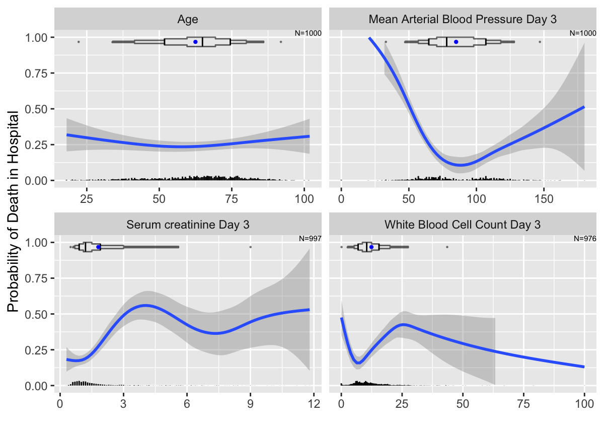

Figure 15.1: `ggplot2` nonparametric smooth estimated relationships between continuous baseline variables and the probability that a patient in the ICU will die in the hospital. Extended box plots are added to the top of the panels, with points added for 0.01 and 0.99 quantiles. Spike histograms are at the bottom. Unlike box plots, spike histograms do not hide the bimodality of mean blood pressure.

Here is a prototype extended box plot to assist interpretation.

bpplt()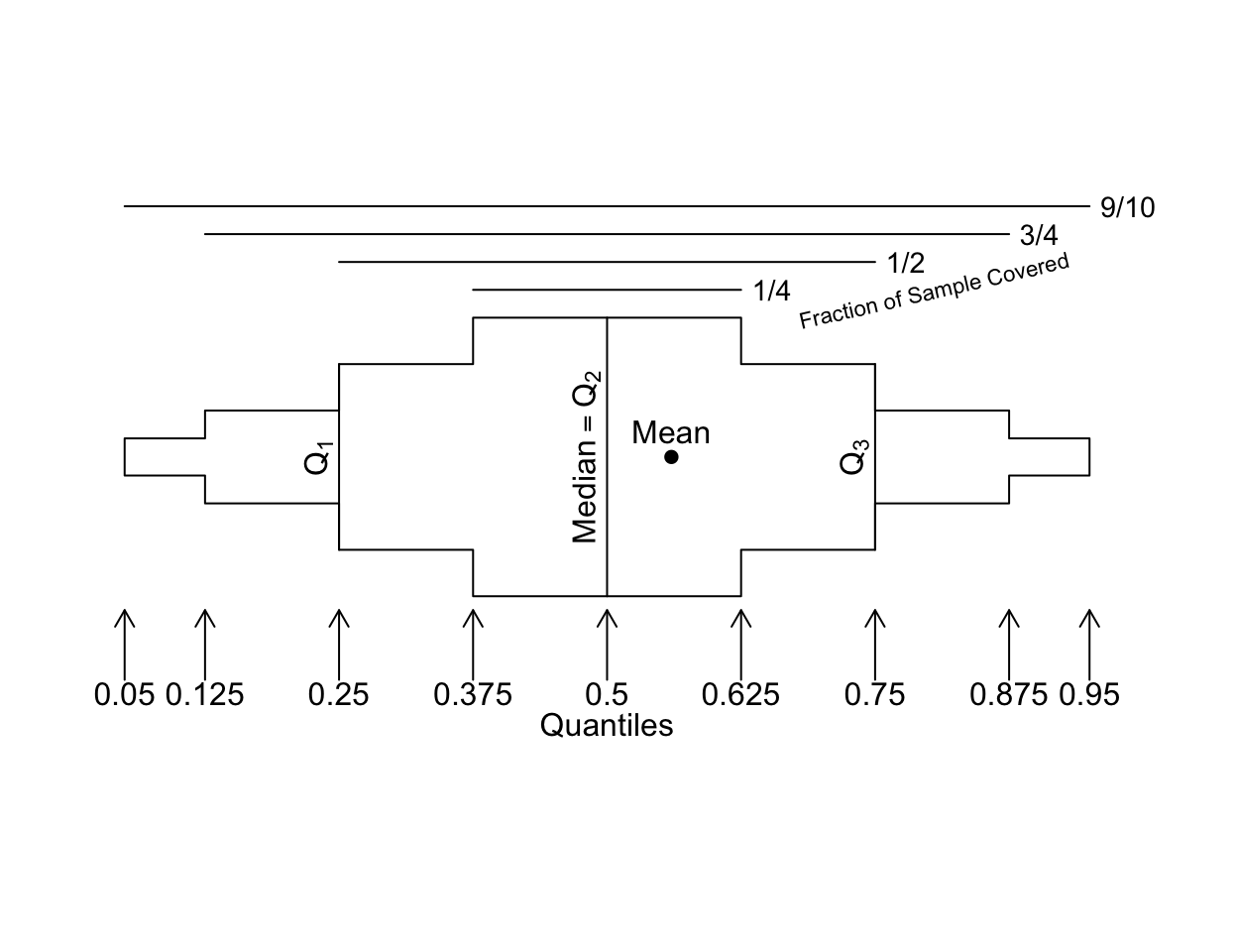

Figure 15.2: Prototype extended box plot

Here are more examples of extended box plots for showing distributions of continuous variables, stratified by disease group.

bpplotM(age + crea + meanbp + wblc ~ dzgroup,
        data=support, cex.strip=0.4, cex.means=0.3, cex.n=0.45)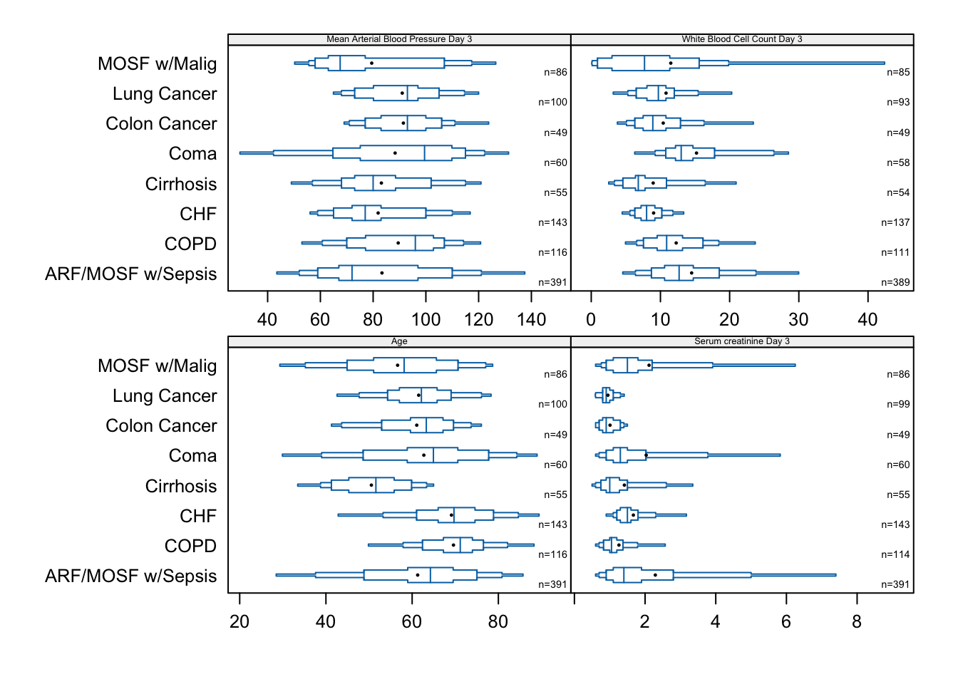

Figure 15.3: `bpplotM` extended box plot examples with stratification by disease group

This is better done with interactive plots so that one can for example hover over a corner of a box plot and see which quantile that corner represents.

s <- summaryM(age + crea + meanbp + wblc ~ dzgroup,
              data=support)
options(grType='plotly')
plot(s)

Figure 15.4: summaryM plotly graphic with interactive extended box plots

15.3 Descriptively Relating One Variable to Another

To understand the relationship between a continuous variable X and an outcome or another variable Y we may estimate the mean, median, and other quantities as a smooth function of X. There are many ways to do this, including

For binary Y the mean is the proportion of ones, which estimates the probability that Y=1

making a scatter plot if Y is continuous or almost continuous
stratifying by fixed or variable intervals of X, e.g., summarizing Y by quintiles of X. This is arbitrary, inefficient, and misleading and should never be done.
using a nonparametric smoother such as loess
parametrically estimating the mean Y as a function of X using an ordinary linear least squares (OLS) model with a regression spline in X so as to not assume linearity
likewise but with a logistic regression model if Y is binary
semiparametrically estimating quantiles of Y as a function of X using quantile regression and a regression spline for X
semiparametrically estimating the mean, quantiles, and exceedance probabilities of Y as a function of X using an ordinal regression model and a spline in X
nonparametrically using overlapping moving windows of X that advance by a small amount each time. For each window compute the estimate of the property of Y using ordinary sample estimators (means, quantiles, Kaplan-Meier estimates, etc.). This approach has the fewest assumptions and is very general in the sense that all types of Y are accommodated. The moving estimates need to be smoothed; the R supsmu function is well suited for this.

The estimated trend curves depend on the window width and amount of smoothing, but this problem is tiny in comparison with the huge effect of changing how a continuous predictor is binned when the usual non-overlapping strata are created. The idea is to assume smooth relationships and get close to the data.

In the following several of the above methods are illustrated to study how serum creatinine of critically ill patients relates to age. Start with a scatterplot that has no problems with ties in the data.

with(support, ggfreqScatter(age, crea))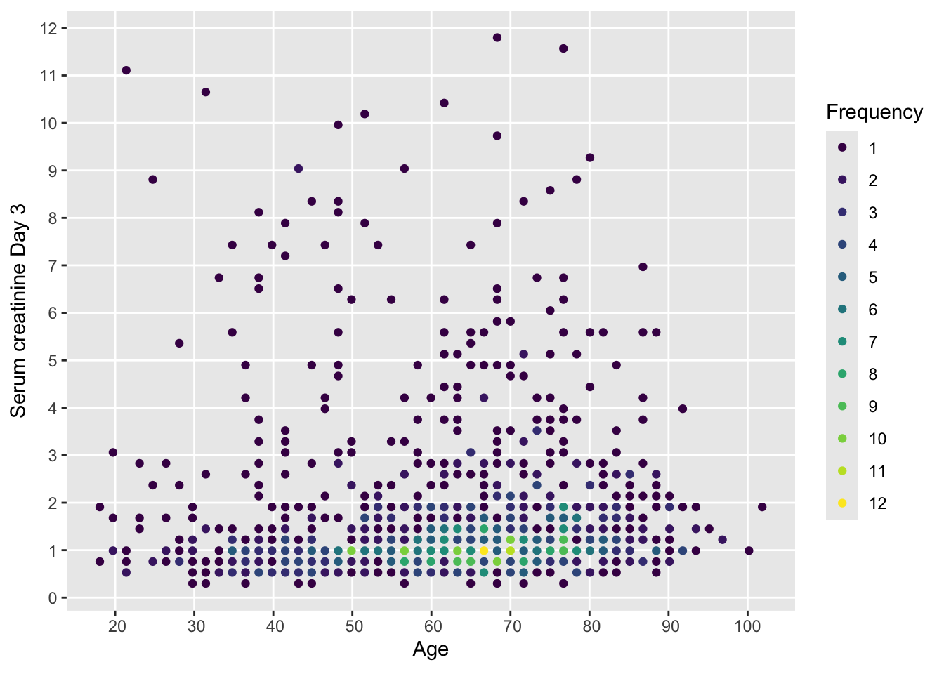

Figure 15.5: `ggfreqScatter` plot showing all raw data for two continuous variables with only slight binning

Now consider moving estimates, least squares (OLS), ordinal regression (ORM), and quantile regression (QR) estimates, nonparametric loess estimates, and a flexible adaptive survival model. Moving estimates computed on overlapping x-variable windows, moving averages being the oldest example, have the advantage of great flexibility. As long as one has an estimator (mean, median, Kaplan-Meier estimate, etc.) that can be applied to a relatively homogeneous (with respect to x) sample, moving statistics can estimate smooth trends over x. Unless the windows are wide or the sample size is very large so that one can afford to use narrow x windows, the moving statistics will be noisy and need to be further smoothed. The smaller the windows, the larger the amount of smoothing will be needed. To control bias it is generally better to have smaller windows and more after-estimation smoothing.

The function movStats in Hmisc provides two methods for creating moving overlapping windows from x. The default used here creates varying-width intervals in the data space but fixed-width in terms of sample size. It includes by default 15 observations to the left of the target point and 15 to the right, and moves up \(\max(\frac{n}{200}, 1)\) observations for each evaluation of the statistics. These may be overridden by specifying eps and xinc. If the user does not provide a statistical estimation function stat, the mean and all three quartiles are estimated for each window. movStats makes heavy use of the data.table, rms, and other packages. For ordinal regression estimates of the mean and quantiles the log-log link is used in the example below. Moving estimates are shown with and without supsmu-smoothing them.

u <- movStats(crea ~ age,
              loess=TRUE, ols=TRUE, qreg=TRUE,
              orm=TRUE, family='loglog', msmooth='both',
              melt=TRUE, data=support, pr='margin')

	Window Sample Sizes
N	Mean	Min	Max	xinc
997	31	25	31	4

# pr='margin' causes window information to be put in margin
ggplot(u, aes(x=age, y=crea, col=Type)) + geom_line() +
  facet_wrap(~ Statistic) +
  xlab('Age') + ylab('Serum Creatinine')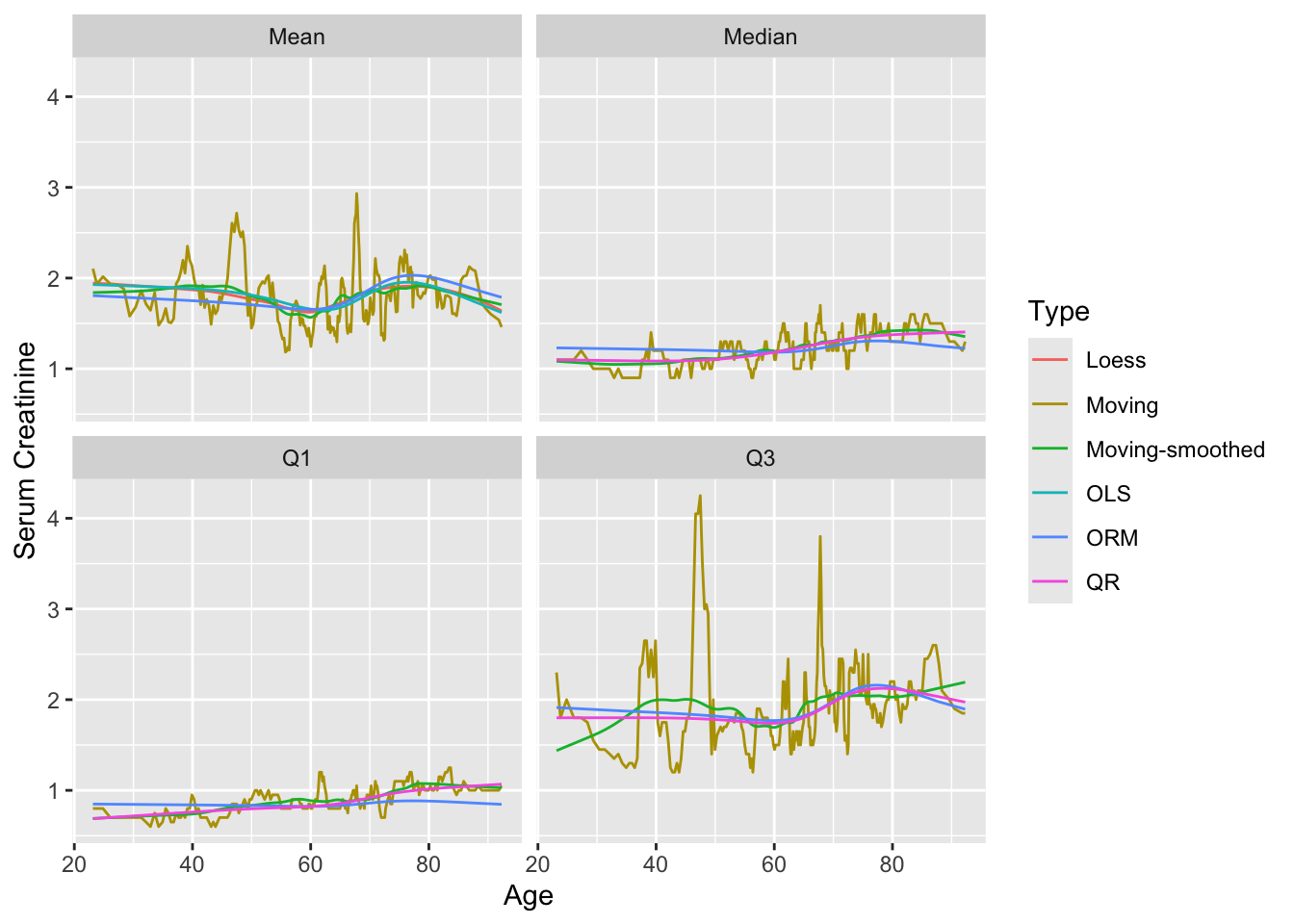

Figure 15.6: `movStats` moving estimates of mean and quantiles of `crea` as a function of `age` using small overlapping windows, with and without smoothing of the moving estimates

Recommended practice for relating a continuous variable to another continuous variable, especially for replacing parts of Table 1 or Table 2, is to use smoothed moving statistics or (1) a spline OLS model to estimate the mean and (2) a spline quantile regression model for estimating quantiles. Here is an example best practice that shows a preferred subset of the estimates from the last plot. melt=TRUE is omitted so we can draw a ribbon to depict the outer quartiles.

u <- movStats(crea ~ age, bass=9, data=support)
ggplot(u, aes(x=age, y=`Moving Median`)) + geom_line() +
  geom_ribbon(aes(ymin=`Moving Q1`, ymax=`Moving Q3`), alpha=0.2) +
  geom_line(aes(x=age, y=`Moving Mean`, col=I('blue'))) +
  xlab('Age') + ylab('Serum Creatinine') +
  labs(caption='Black line: median\nBlue line: mean\nBand: Q1 & Q3')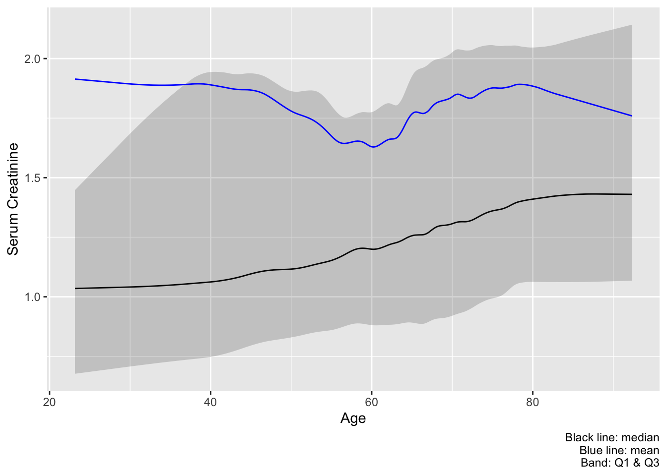

Figure 15.7: Moving mean and quantile estimates of effect of `age` with interquartile bands

Let’s describe how white blood count relates to the probability of hospital death, using a binary logistic regression model and moving proportions. The cube root transformation in regression fits is used because of the extreme skewness of WBC. Use 6 knots at default locations on \(\sqrt[3]{\mathrm{WBC}}\). The \(\sqrt[3]{\mathrm{WBC}}\) transformation affects moving statistics only in that mean x-values for plotting are cubes of mean \(\sqrt[3]{\mathrm{WBC}}\) instead of means on the original WBC scale.

u <- movStats(hospdead ~ wblc, k=6, eps=20, bass=3,
              trans  = function(x) x ^ (1/3),
              itrans = function(x) x ^ 3,
              loess=TRUE, lrm=TRUE, msmooth='both',
              melt=TRUE, pr='margin', data=support)

	Window Sample Sizes
N	Mean	Min	Max	xinc
976	40.8	30	41	4

ggplot(u, aes(x=wblc, y=hospdead, col=Type)) + geom_line() +
  guides(color=guide_legend(title='')) +
  theme(legend.position='bottom')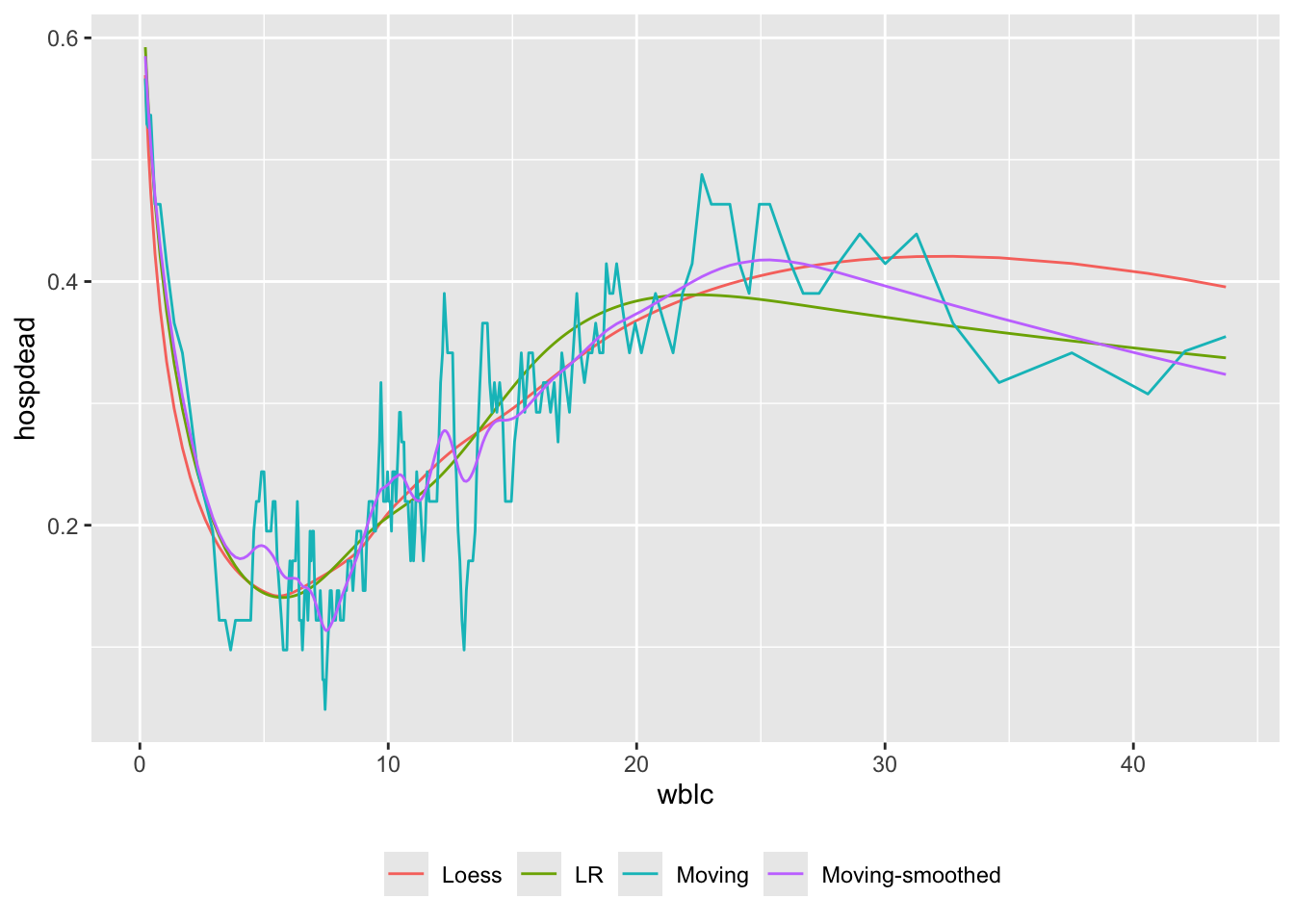

Figure 15.8: Moving estimates of the relationship between white blood count and hospital mortality, using a \(\sqrt[3]{}\) transformation to make the WBC distribution more symmetric

The flexibility of the moving statistic method is demonstrated by estimating how age relates to probabilities of death within 1y and within 2y using Kaplan-Meier estimates in overlapping moving windows. Assumptions other than smoothness (e.g., proportional hazards) are avoided in this approach. Here is an example that also uses an flexible parametric method, hazard regression, implemented in the R polspline package, that adaptively finds knots (points of slope change) in the covariate and in time, and products of piecewise linear terms so as to allow for non-proportional hazards. We use far less penalization than is the default for the hare function for demonstration purposes. For this dataset the default settings of penalty and maxdim result in straight lines.

require(survival)  # needed for Surv; could also do survival::Surv
u <- movStats(Surv(d.time / 365.25, death) ~ age, times=1:2,
              eps=30, bass=9,
              hare=TRUE, penalty=0.5, maxdim=30,
              melt=TRUE, data=support)
ggplot(u, aes(x=age, y=incidence, col=Statistic)) + geom_line() +
  facet_wrap(~ Type) +
  ylab(label(u$incidence)) +
  guides(color=guide_legend(title='')) +
  theme(legend.position='bottom')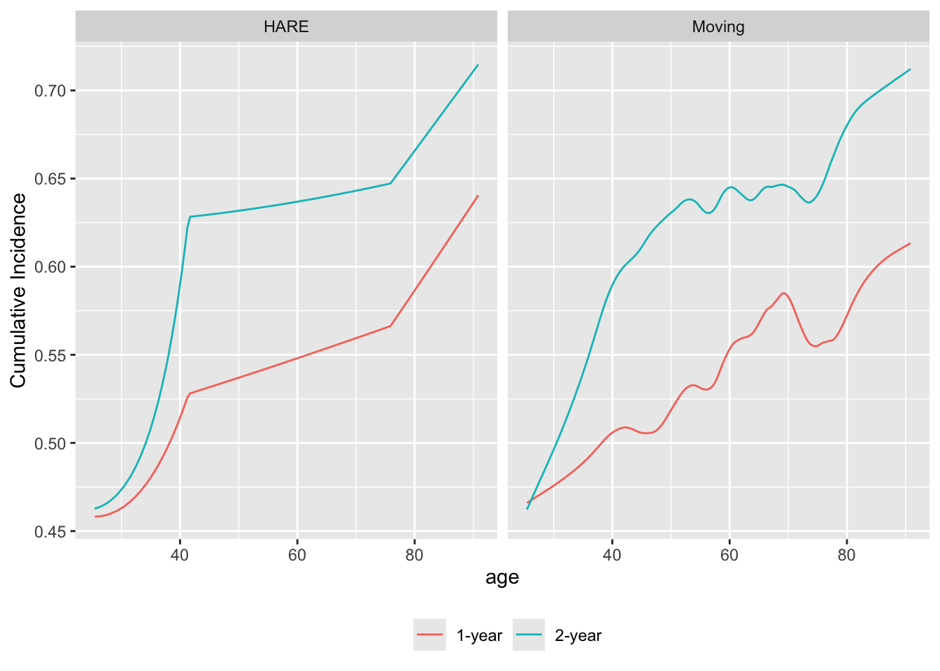

Figure 15.9: Moving one minus Kaplan-Meier and HARE estimates estimating the relationship between `age` and the probability of dying by 1y and by 2y

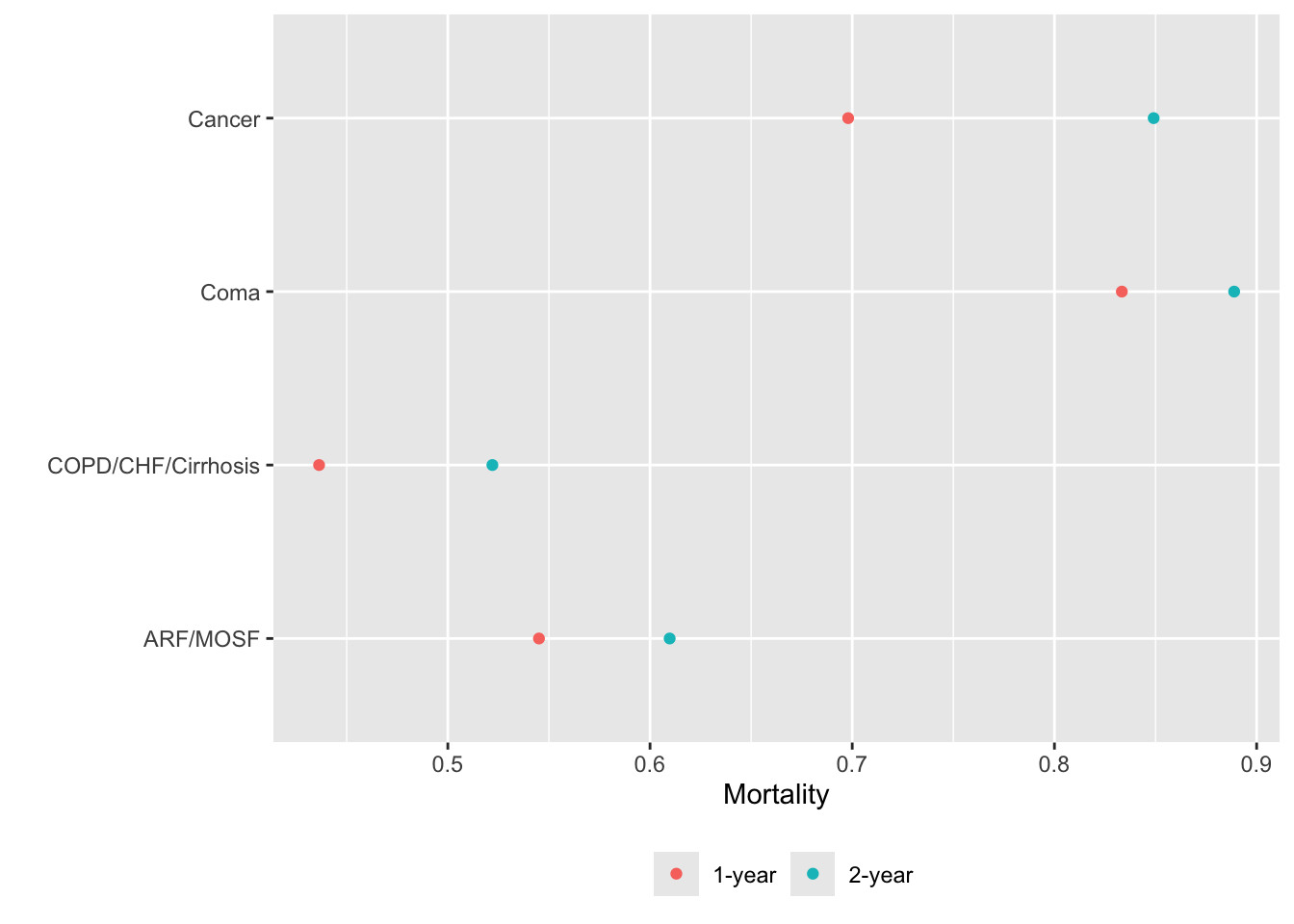
movStats can also compute stratified non-smoothed estimates when x is discrete. After computing 1- and 2y Kaplan-Meier incidence probability estimates, order disease groups by ascending order of 1-year mortality before plotting.

u <- movStats(Surv(d.time / 365.25, death) ~ dzgroup, times=1:2,
              discrete=TRUE,
              melt=TRUE, data=support)
m1 <- u[Statistic == '1-year', .(dzgroup, incidence)]
i  <- m1[, order(incidence)]
u[, dzgroup := factor(dzgroup, levels=m1[i, dzgroup])]
ggplot(u, aes(x=incidence, y=dzgroup, col=Statistic)) + geom_point() +
  xlab(label(u$incidence)) + ylab('') +
  guides(color=guide_legend(title='')) +
  theme(legend.position='bottom')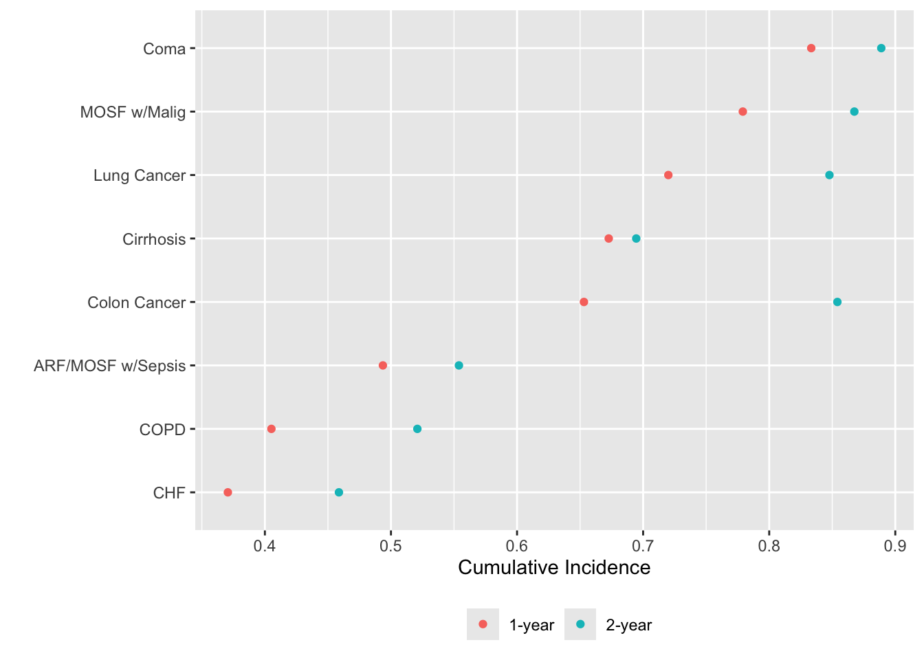

Figure 15.10: Ordinary incidence estimates stratified by disease group, with groups ordered by 1-year mortality estimates

15.4 One Continuous and One Categorical Predictor

It is possible to descriptively estimate trends against more than one independent variables when the effective sample size is sufficient. Trends can be estimated nonparametrically through stratification (when the third variable is categorical) or with flexible regression models allowing the two predictors to interact. In the graphical displays it is useful to keep sample size limitations in certain regions of the space defined by the two predictors in mind, by superimposing spike histograms on trend curves.

Repeat the last example but stratified by disease class. The window is widened a bit because of the reduced sample size upon stratification. Default smoothing is used for hazard regression.

# The Coma stratum has only n=60 so is not compatible with eps=75
# Use varyeps options
u <- movStats(Surv(d.time / 365.25, death) ~ age + dzclass, times=1:2,
              eps=30,
              msmooth='both', bass=8, hare=TRUE,
              melt=TRUE, data=support, pr='margin')

		Window Sample Sizes
	N	Mean	Min	Max	xinc
ARF/MOSF	477	59.9	40	61	2
COPD/CHF/Cirrhosis	314	59.4	40	61	1
Coma	60	50.0	40	60	1
Cancer	149	57.5	40	61	1

ggplot(u, aes(x=age, y=incidence, col=dzclass)) + geom_line() +
  facet_grid(Type ~ Statistic) +
  ylab(label(u$incidence)) +
  guides(color=guide_legend(title='')) +
  theme(legend.position='bottom')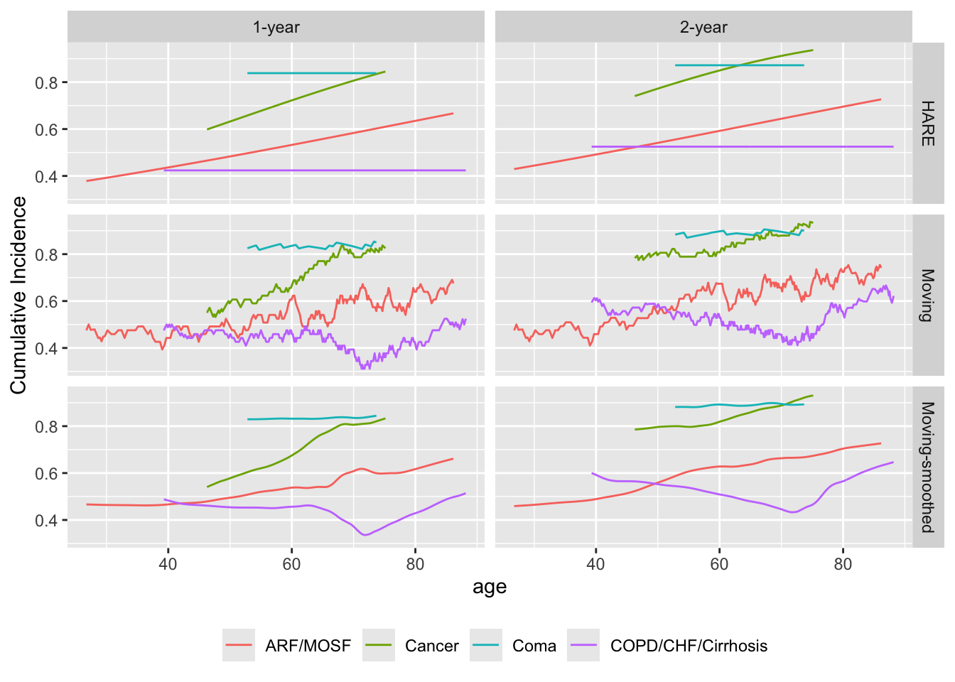

Figure 15.11: Moving Kaplan-Meier (smoothed and unsmoothed) and HARE estimates of the age effect on time to death, stratified by disease class

Consider another example with a continuous dependent variable. Use the NHANES dataset that was created for analyzing glycohemoglobin (HbA\(_{\mathrm{1c}}\)) for diabetes screening. Stratify by race/ethnicity

getHdata(nhgh)
u <- movStats(gh ~ age + re,
              melt=TRUE, data=nhgh, pr='margin')

		Window Sample Sizes
	N	Mean	Min	Max	xinc
Mexican American	1366	31.0	25	31	6
Other Hispanic	706	30.9	25	31	3
Non-Hispanic White	3117	31.0	25	31	15
Non-Hispanic Black	1217	31.0	25	31	6
Other Race Including Multi-Racial	389	30.9	25	31	1

ggplot(u, aes(x=age, y=gh, col=re)) + geom_line() +
  facet_wrap( ~ Statistic) +
  ylab(label(nhgh$gh)) +
  guides(color=guide_legend(title='', nrow=2)) +
  theme(legend.position='bottom')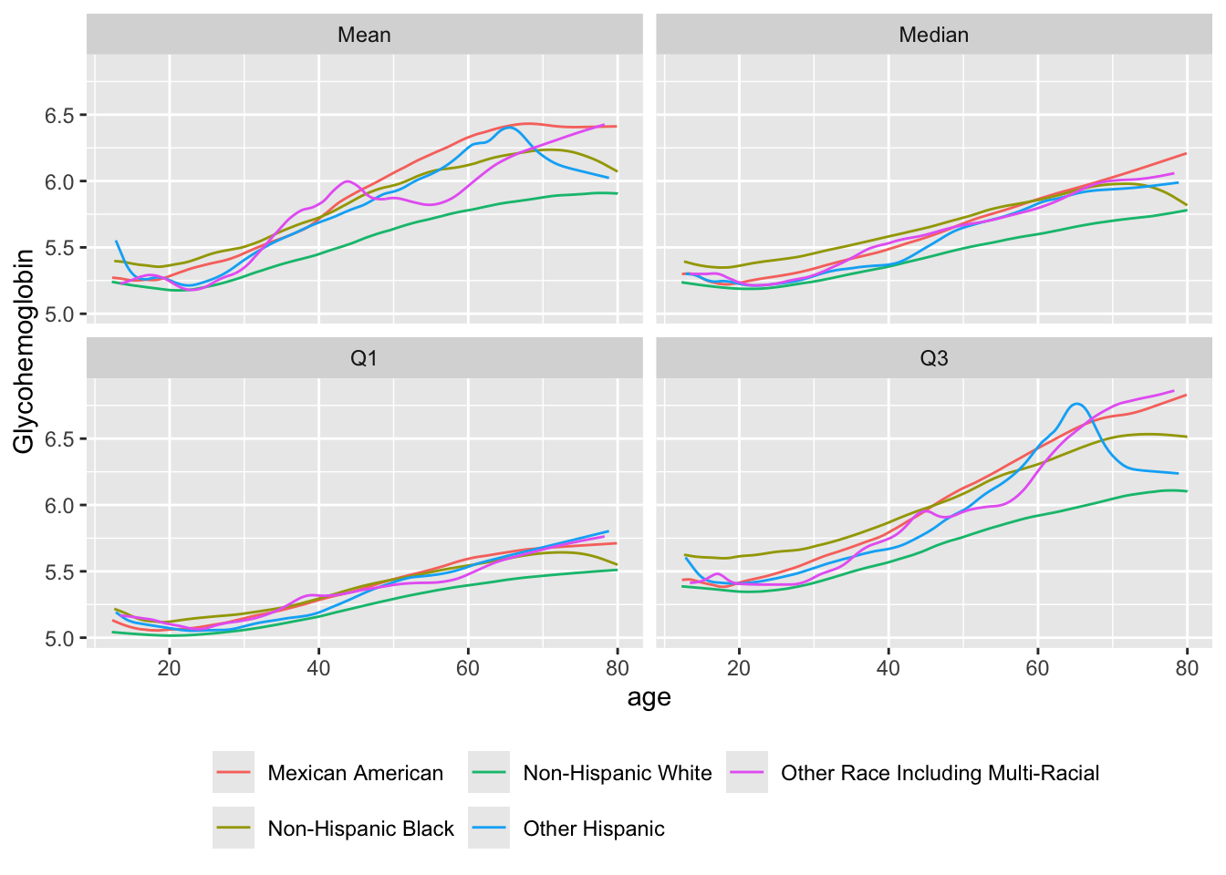

Figure 15.12: Moving estimates of effect of age on glycohemoglobin stratified by race/ethnicity

Mimic these results using flexible regression with interaction. Start by estimating the mean. Add spike histograms to estimated trend curves. Spike heights are proportional to the sample size in age/race-ethnicity groups after binning age into 100 bins. Direct plotly plotting is used. The user can click on elements of the legend (including the histograms) to turn their display off and on.

require(rms)
options(prType='html')  # needed to use special formatting (can use prType='latex')
dd <- datadist(nhgh); options(datadist='dd')
f <- ols(gh ~ rcs(age, 5) * re, data=nhgh)
# fontsize will be available for print(anova()) in rms 6.3-1
makecolmarg(anova(f), dec.ms=2, dec.ss=2, fontsize=0.6)

	d.f.	Partial SS	MS	F	P
Analysis of Variance for `gh`
age (Factor+Higher Order Factors)	20	878.06	43.90	55.20	<0.0001
All Interactions	16	42.55	2.66	3.34	<0.0001
Nonlinear (Factor+Higher Order Factors)	15	61.26	4.08	5.13	<0.0001
re (Factor+Higher Order Factors)	20	169.42	8.47	10.65	<0.0001
All Interactions	16	42.55	2.66	3.34	<0.0001
age × re (Factor+Higher Order Factors)	16	42.55	2.66	3.34	<0.0001
Nonlinear	12	14.62	1.22	1.53	0.1051
Nonlinear Interaction : f(A,B) vs. AB	12	14.62	1.22	1.53	0.1051
TOTAL NONLINEAR	15	61.26	4.08	5.13	<0.0001
TOTAL NONLINEAR + INTERACTION	19	101.38	5.34	6.71	<0.0001
REGRESSION	24	937.86	39.08	49.13	<0.0001
ERROR	6770	5384.94	0.80

# Normal printing: anova(f) or anova(f, dec.ms=2, dec.ss=2)
hso <- list(frac=function(f) 0.1 * f / max(f),
            side=1, nint=100)
# Plot with plotly directly
plotp(Predict(f, age, re), rdata=nhgh, histSpike.opts=hso)

Figure 15.13: Predicted mean glycohemoglobin as a function of age and race/ethnicity, with age modeled as a restricted cubic spline with 5 default knots, and allowing the shape of the age effect to be arbitrarily different for the race/ethnicity groups

Now use quantile regression to estimate quartiles of glycohemoglobin as a function of age and race/ethnicity.

f1 <- Rq(gh ~ rcs(age, 5) * re, tau=0.25, data=nhgh)
f2 <- Rq(gh ~ rcs(age, 5) * re, tau=0.5,  data=nhgh)
f3 <- Rq(gh ~ rcs(age, 5) * re, tau=0.75, data=nhgh)
p  <- rbind(Q1     = Predict(f1, age, re, conf.int=FALSE),
            Median = Predict(f2, age, re, conf.int=FALSE),
            Q3     = Predict(f3, age, re, conf.int=FALSE))
ggplot(p, histSpike.opts=hso)

Figure 15.14: Smooth age effects on three quartiles of HbA\(_{1c}\)

15.5 Another Replacement for Table 1

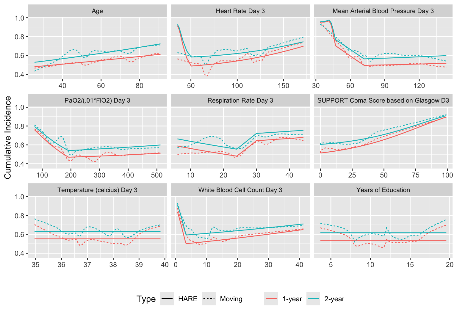
We can create a matrix of plots that respect continuous baseline variables while staying close to the data through the use of overlapping moving windows. In the following example we compute moving 1y and 2y mortality for selected continuous baseline variables in support and stack them together. Flexible HARE hazard regression estimates are also included.

qreport includes a function varType to determine the continuous/discrete nature of each variable, and other functions that make it easy to extract the list of either continuous variables (conVars) or discrete variables (disVars). varType also has a third classification: non-numeric variables that have too many (by default > 20) distinct values to be considered discrete.

# Exclude outcome variables from consideration
outcomes <- .q(slos, charges, totcst, totmcst, avtisst,
               d.time, death, hospdead, sfdm2)
types <- varType(support, exclude=outcomes)
print(types, quote=FALSE)

$continuous
 [1] age     edu     scoma   meanbp  wblc    hrt     resp    temp    pafi   
[10] alb     bili    crea    sod     ph      glucose bun     urine   adlsc  

$discrete
[1] sex     dzgroup dzclass num.co  income  race    adlp    adls

Let’s use only the first 9 continuous variables. In addition to showing all the estimated relationships with the outcome, put covariate distributions in collapsed note. Note the bimodality of some of the measurements, and true zero blood pressures for patients having cardiac arrest.

V <- types$continuous[1:9]
U <- list()
for(v in V) {
  x <- support[[v]]
  u <- movStats(Surv(d.time / 365.25, death) ~ x, times=1:2,
              eps=30, hare=TRUE, penalty=0.25, maxdim=10,
              msmooth='smoothed', bass=8,
              melt=TRUE, data=support)
  U[[label(x, default=v)]] <- u  # stuffs u in an element of list U
                                 # & names the element w/ var label/name
}
w <- rbindlist(U, idcol='vname')   # stack all the data tables
ggplot(w, aes(x, y=incidence, col=Statistic, linetype=Type)) + geom_line() +
  facet_wrap(~ vname, scales='free_x') +
  ylab(label(u$incidence)) + xlab('') +
  guides(color=guide_legend(title='')) +
  theme(legend.position='bottom',
        strip.text = element_text(size=8))
makecnote(`Covariate Distributions` ~ plot(describe(support[, ..V])))

Covariate Distributions

Figure 15.15: Moving Kaplan-Meier and HARE estimates of a series of continuous covariate effects stacked into one `ggplot2` graphic

If we were not showing main graphs in wide format (using a Quarto callout) we could have put the marginal distributions in the right margin using the following, which shrinks the plotly output.

require(plotly)   # for %>%
pl <- plot(describe(support[, ..V])) %>%
        layout(autosize=FALSE, width=350, height=325)
makecolmarg(~ pl)

Likewise we can produce a graph summarizing how categorical baseline variables relate to the study outcome variable.

V <- types$discrete   # or disVars(support, exclude=...)
U <- list()
for(v in V) {
  x <- support[[v]]
  u <- movStats(Surv(d.time / 365.25, death) ~ x, times=1:2,
                discrete=TRUE, melt=TRUE, data=support)
  U[[label(x, default=v)]] <- u
}
w <- rbindlist(U, idcol='vname')   # stack the tables
ggplot(w, aes(x=incidence, y=x, col=Statistic)) + geom_point() +
  facet_wrap(~ vname, scales='free_y') +
  xlab(label(u$incidence)) + ylab('') +
  guides(color=guide_legend(title='')) +
  theme(legend.position='bottom')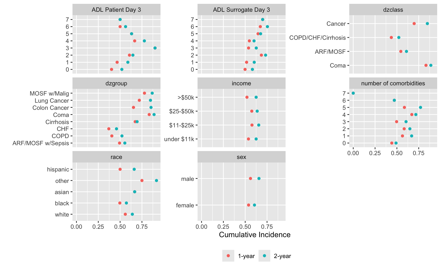

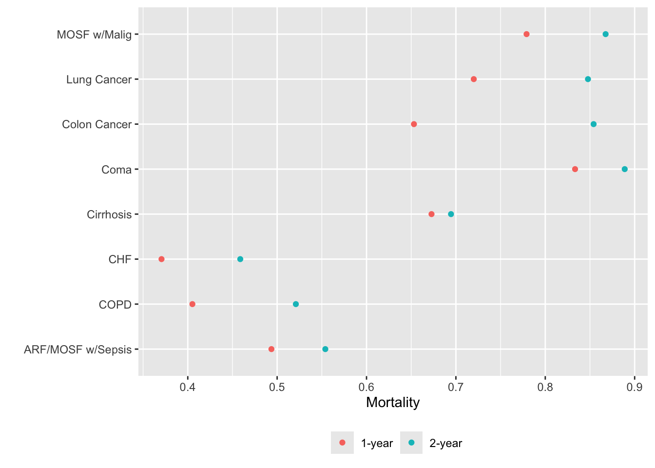
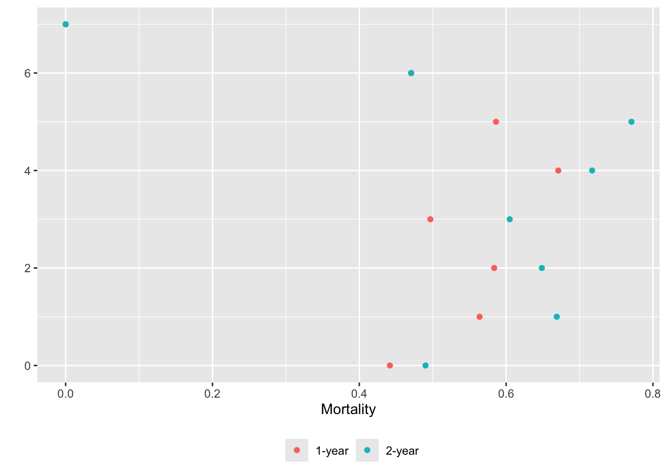
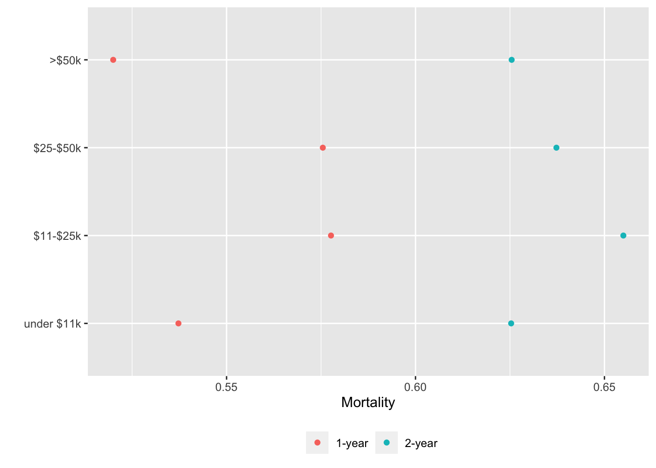
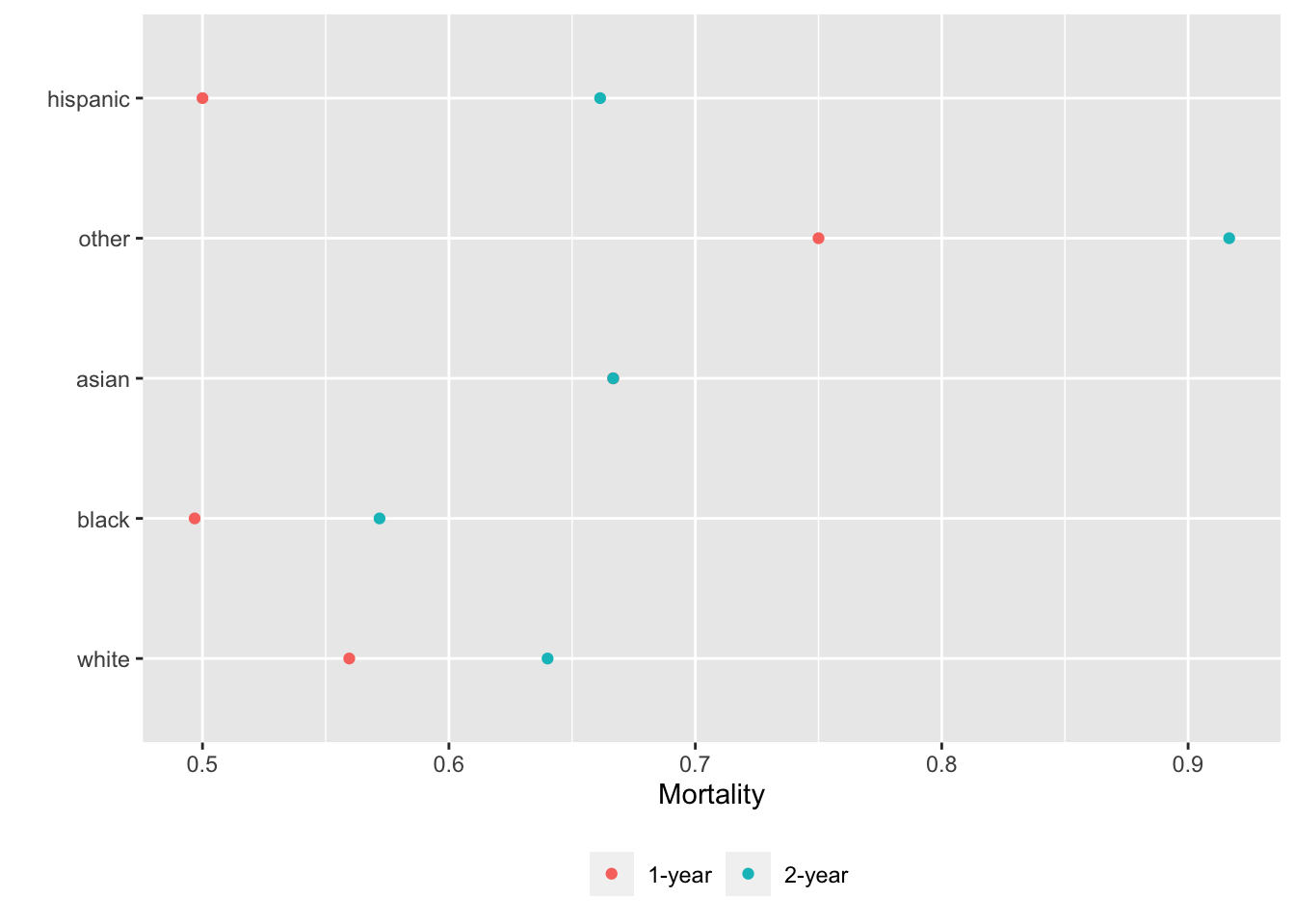
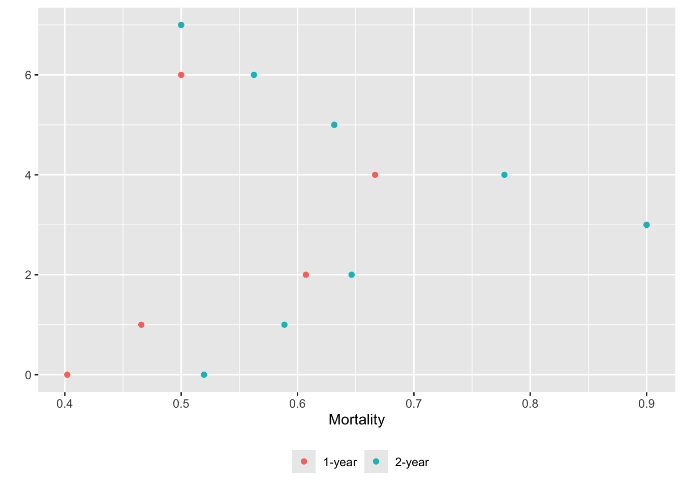
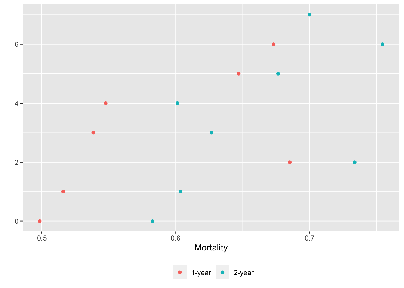
Figure 15.16: Kaplan-Meier estimates of 1y and 2y incidence stratified separately by a series of discrete predictorsw

Alternatively we can put each variable in a separate tab:

gg <- function(data)
  ggplot(data, aes(x=incidence, y=x, col=Statistic)) + geom_point() +
    xlab('Mortality') + ylab('') +
    guides(color=guide_legend(title='')) +
    theme(legend.position='bottom')
g <- lapply(U, gg)       # one ggplot per element (a data table) in U
maketabs(g, cap=1,
  basecap='Kaplan-Meier estimates of 1y and 2y incidence with each predictor in its own tab')

Figure 15.17: Kaplan-Meier estimates of 1y and 2y incidence with each predictor in its own tab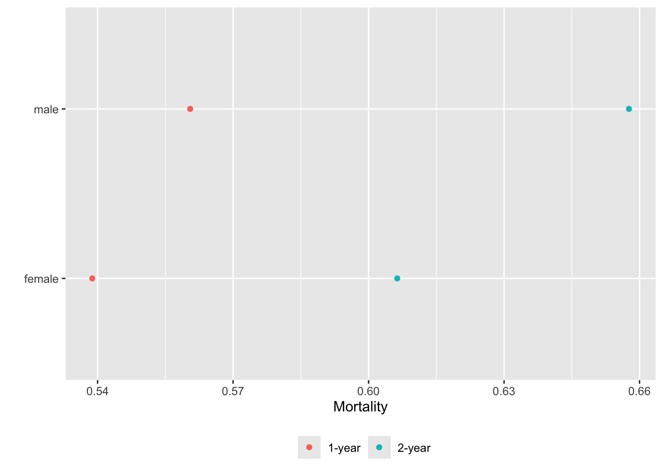

15.6 Confidence Bands for Differences

Studies almost never randomly sample from a population, hence inference to the population for a single treatment’s outcome should seldom be attempted. The uncertainty intervals and bands that should be presented are ones having inferential meaning and are based on treatment differences. One can easily construct a graph that shows differences and confidence intervals for them, but it is useful to be able to show the individual group estimates along with CIs for the differences. Fortunately, Maarten Boers had the idea of a null bar or null zone. When a confidence interval for a difference is symmetric, the confidence interval includes 0.0 if and only if the midpoint of the two outcome estimates \(\pm \frac{1}{4} \times w\) touches the individual group estimates, where \(w\) is the width of the confidence interval. Null zone/half-width CIs can be put to especially good use in avoiding clutter when displaying Kaplan-Meier plots, and can be graphed using the rms package survplot (static plot) and survplotp (plotly interactive graphic) functions. The latter has the additional advantage of providing continuous data on number of subjects still at risk by hovering over the survival curve for one group. Here is an example using support. Estimate survival differences between patients who were or were not able to be interviewed for determining their baseline activities of daily living.

The primary reason for not being interviewed was the patient needing to be on a ventilator.

Cumulative incidence are recommended over cumulative survival probabilities, principally because many journals will force you to scale the \(y\)-axis for survival probability as \([0,1]\) even in a very low-risk sample, whereas journals do not have silly scaling conventions for cumulative incidence.

require(rms)
s <- support[, .(d.time      = d.time / 365.25,
                 death,
                 interviewed = ifelse(is.na(adlp), 'not interviewed',
                                                   'interviewed'))]
units(s$d.time) <- 'year' 
# Compute nonparametric Kaplan-Meier estimates (uses survival::survfit)
f <- npsurv(Surv(d.time, death) ~ interviewed, data=s)
survplotp(f, fun=function(y) 1. - y)

Figure 15.18: Interactive survival curves with half-width confidence bands

Hovering over the curves reveals the continuous number at risk. Non-recommended individual survival curves can be turned on by clicking in the legend, and the null zone bands can be turned off. Note strong evidence for a difference in mortality early but not as much late.

To produce an additional .pdf graphic in a separate file, with the number of risk shown below the graph, run the following. Add include=FALSE in the chunk header if you want to show no trace of this chunk in the report.

pdf('survplot.pdf')
survplot(f, fun=function(y) 1. - y, conf='diffbands',
         ylab='Cumulative Mortality', levels.only=TRUE,
         n.risk=TRUE, time.inc=1, label.curves=list(keys='lines'))
dev.off()

The adverse event chart in ?fig-aeplot is another example using half-width confidence intervals.

15.7 Third-Order Descriptive Analysis

We have seen univariate and associative analysis examples up until now. Consider an example of a third-order analysis in which we examine whether and how the association between two variables \(X\) and \(Y\) changes over levels of a third variable \(Z\). The dataset was donated by a pharmaceutical company and comes from combining three double-masked placebo-controlled Phase III randomized studies. A variety of drug safety parameters were assessed at multiple times (weeks 0, 2, 4, 8, 12, 16, 20), including adverse events, vital signs, hematology, clinical chemistry, and ECG data. Subjects were randomized 2:1 drug:placebo (\(n=1374\) and \(684\)). More in-depth analysis may be found here.

This could be called a third-order nonparametric descriptive analysis. A formal third-order analysis would be more parametric in nature, perhaps utilizing third-order interactions \(X \times Y \times Z\) if we were relating baseline variables \(X,Y,Z\) to an ultimate response variable. But our example entails changes in relationships between two (at a time) response variables as a function of time.

Our goal is to describe whether the degree of coupling of clinical chemistry and hematology parameters changes over time. A Spearman \(\rho\) rank correlation matrix is estimated on all pairs of clinical chemistry and hematology variables, separately at each time \(t\). Then the rank correlations are rank correlated with \(t\) to estimate changes in associations over time. Such a third-order analysis might find that early after beginning treatment, the lab measurements are varying more independently, but as the trial progresses these parameters may begin to move together. We consider here only subjects on the active drug.

The safety dataset is on hbiostat.org/data and is fetched using Hmisc::getHdata.

getHdata(safety)
d <- All            # safety was created using save() and had
setDT(d, key='week')            # an original name of All
d <- d[trx == 'Drug']
# Get a vector of names of lab variables we want to analyze
# Start with a larger list, the remove some variables
vars <- setdiff(names(d)[16:48],
               .q(amylase,aty.lymph,glucose.fasting,neutrophil.bands,
                  lymphocytes.abs,monocytes.abs,
                  neutrophils.seg,eosinophils.abs,basophils.abs))
print(vars, quote=FALSE)

 [1] neutrophils alat        albumin     alk.phos    asat        basophils  
 [7] bilirubin   bun         chloride    creatinine  eosinophils ggt        
[13] glucose     hematocrit  hemoglobin  potassium   lymphocytes monocytes  
[19] sodium      platelets   protein     rbc         uric.acid   wbc

For each week, compute the minimum and maximum number of non-NA values over all lab parameters, and identify which variables had those frequencies.

g <- function(x) {
  m <- sapply(x, function(y) sum(! is.na(y)))
  mn <- m[which.min(m)]
  mx <- m[which.max(m)]
  # g returns a list of lists; data.table will make columns Lowest,Highet
  # and will print 2 rows for each week (one with variable names, one w/N)
  list(Lowest=list(names(mn), mn), Highest=list(names(mx), N=mx))
}
d[, g(.SD), by=week, .SDcols=vars]

    week      Lowest     Highest
 1:    0   basophils    chloride
 2:    0         425        1362
 3:    1 neutrophils neutrophils
 4:    1           0           0
 5:    2   basophils  hematocrit
 6:    2         377        1240
 7:    4   basophils    chloride
 8:    4         357        1204
 9:    8   basophils    chloride
10:    8         335        1129
11:   12   basophils  hematocrit
12:   12         315        1071
13:   16   basophils        alat
14:   16          12          27
15:   20   basophils        alat
16:   20           4          14

Lab data collection essentially stopped after week 12, and lab values were not collected at week 1. So limit the weeks being analyzed.

wks <- c(0, 2, 4, 8, 12)
# For each time compute the correlation matrix and stuff it into a 3-dimensional array
p   <- length(vars)
k   <- length(wks)
r   <- array(NA, c(p, p, k), list(vars, vars, as.character(wks)))
dim(r)

[1] 24 24  5

for(w in wks) {
  # Compute correlation matrix for week w using pairwise deletion
  m=d[week==w, cor(.SD, use='pairwise.complete.obs', method='spearman'),
      .SDcols=vars]
  r[, , as.character(w)] <- m
  # Omitting a dimension means "use all elements of that dimension"
}
# For each pair of variables compute Spearman correlation with week
R <- r[, , 1]   # use one time point in array as storage prototype
for(i in 1 : (p - 1))
  for(j in (i + 1) : p)
    # r[i, j, ] is a k-vector of rhos over time for vars[i] and vars[j]
    # omitting third subscript of r means "use all times"
    R[i, j] <- cor(r[i, j, ], wks, method='spearman')
# Set mirror image to avoid duplicate computations
R[upper.tri(R)] <- R[lower.tri(R)]
# Use the Hmisc plotCorrM function to visualize matrix
# Use only the first graphic produced
plotCorrM(R, xangle=90)[[1]]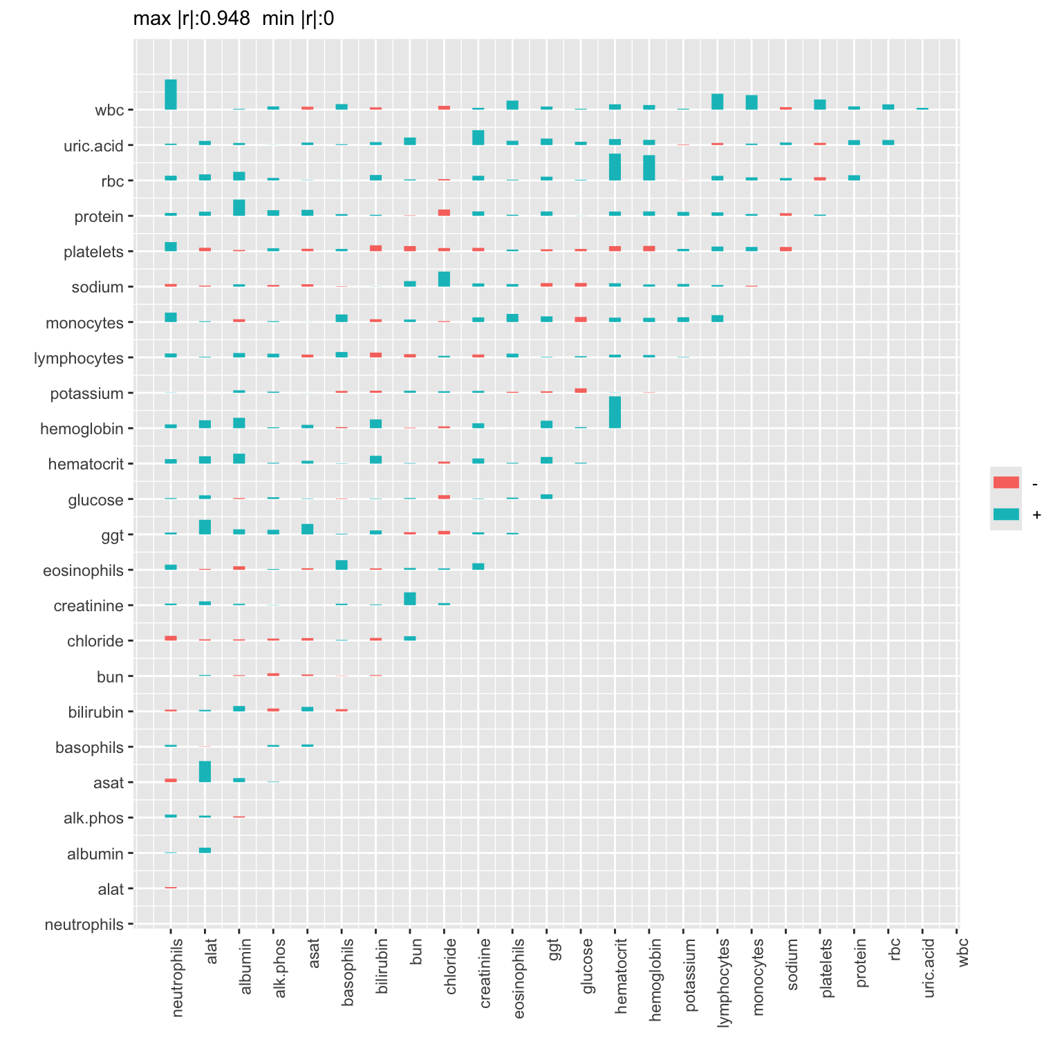

Figure 15.19: Spearman correlations between pairwise clinical chemistry/hematology variable correlations and time

The correlations that are large in absolute value tended to be positive (blue). Positive correlations imply that the indicated pair of variables became more positively correlated over time. This is especially the case for the association between white blood count and neutrophil count, liver enzymes alat and asat, and for correlations involving red blood cell count, hemoglobin, and hematocrit.

Beware that some pairs had low sample sizes.

15.8 Formatting

I take advantage of special formatting for model fit objects from the rms package by using html or latex methods and putting results='asis' in the chunk header to preserve the formatting.

require(rms)
options(prType='html')  # needed to use special formatting (can use prType='latex')
dd <- datadist(support); options(datadist='dd') # rms needs for summaries, plotting
cr <- function(x) x ^ (1/3)
f <- lrm(hospdead ~ rcs(meanbp, 5) + rcs(age, 5) + rcs(cr(crea), 4), data=support)
f

Logistic Regression Model

lrm(formula = hospdead ~ rcs(meanbp, 5) + rcs(age, 5) + rcs(cr(crea), 
    4), data = support)

Frequencies of Missing Values Due to Each Variable

hospdead   meanbp      age     crea 
       0        0        0        3

	Model Likelihood Ratio Test	Discrimination Indexes	Rank Discrim. Indexes
Obs 997	LR χ² 184.06	R² 0.249	C 0.758
0 744	d.f. 11	R²_11,997 0.159	D_xy 0.515
1 253	Pr(>χ²) <0.0001	R²_11,566.4 0.263	γ 0.516
max \|∂log L/∂β\| 5×10^-12		Brier 0.153	τ_a 0.195

	β	S.E.	Wald Z	Pr(>\|Z\|)
Intercept	11.2198	2.2071	5.08	<0.0001
meanbp	-0.1020	0.0212	-4.81	<0.0001
meanbp'	0.1929	0.1766	1.09	0.2749
meanbp''	-0.1286	0.6715	-0.19	0.8481
meanbp'''	-0.2329	0.6487	-0.36	0.7196
age	-0.0152	0.0209	-0.73	0.4678
age'	0.0003	0.0802	0.00	0.9968
age''	0.1889	0.5300	0.36	0.7216
age'''	-0.5770	1.2262	-0.47	0.6380
crea	-6.3192	1.8831	-3.36	0.0008
crea'	83.8882	17.6618	4.75	<0.0001
crea''	-196.2020	40.5695	-4.84	<0.0001

makecnote(anova(f))   # in collapsible note

anova(f)

	χ²	d.f.	P
Wald Statistics for `hospdead`
meanbp	78.98	4	<0.0001
Nonlinear	63.70	3	<0.0001
age	2.86	4	0.5817
Nonlinear	2.78	3	0.4275
crea	46.03	3	<0.0001
Nonlinear	24.52	2	<0.0001
TOTAL NONLINEAR	90.53	8	<0.0001
TOTAL	131.57	11	<0.0001

Write a function to compute several rms package model summaries and put them in tabs. raw in a formula makes the generated R chunk include output in raw format.

rmsdisplay <- function(f) {
  .f. <<- f  # save in global environment so generated chunks have access to it
  maketabs(
    ` `              ~ ` `,
    Model            ~ .f.,
    Specs            ~ specs(.f., long=TRUE) + raw,
    Equation         ~ latex(.f.),
    ANOVA            ~ anova(.f.) + plot(anova(.f.)),
    ORs              ~ plot(summary(.f.), log=TRUE, declim=2) +
                           caption('Graphical representations of a fitted binary logistic model'),
   `Partial Effects` ~ ggplot(Predict(.f.)),
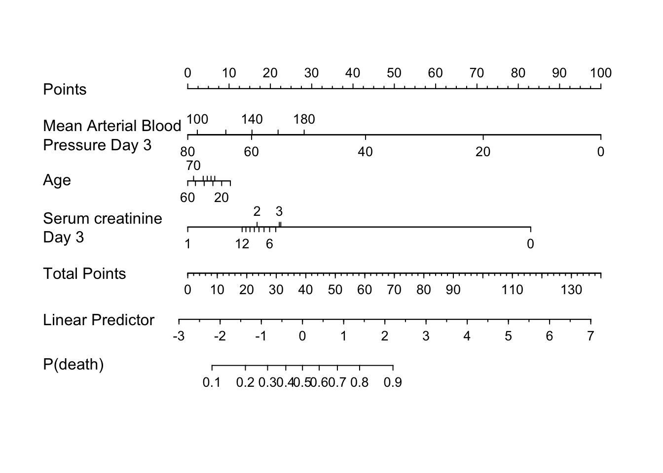
    Nomogram         ~ plot(nomogram(.f., fun=plogis, funlabel='P(death)')))
}

rmsdisplay(f)

Logistic Regression Model

lrm(formula = hospdead ~ rcs(meanbp, 5) + rcs(age, 5) + rcs(cr(crea), 
    4), data = support)

Frequencies of Missing Values Due to Each Variable

hospdead   meanbp      age     crea 
       0        0        0        3

	Model Likelihood Ratio Test	Discrimination Indexes	Rank Discrim. Indexes
Obs 997	LR χ² 184.06	R² 0.249	C 0.758
0 744	d.f. 11	R²_11,997 0.159	D_xy 0.515
1 253	Pr(>χ²) <0.0001	R²_11,566.4 0.263	γ 0.516
max \|∂log L/∂β\| 5×10^-12		Brier 0.153	τ_a 0.195

	β	S.E.	Wald Z	Pr(>\|Z\|)
Intercept	11.2198	2.2071	5.08	<0.0001
meanbp	-0.1020	0.0212	-4.81	<0.0001
meanbp'	0.1929	0.1766	1.09	0.2749
meanbp''	-0.1286	0.6715	-0.19	0.8481
meanbp'''	-0.2329	0.6487	-0.36	0.7196
age	-0.0152	0.0209	-0.73	0.4678
age'	0.0003	0.0802	0.00	0.9968
age''	0.1889	0.5300	0.36	0.7216
age'''	-0.5770	1.2262	-0.47	0.6380
crea	-6.3192	1.8831	-3.36	0.0008
crea'	83.8882	17.6618	4.75	<0.0001
crea''	-196.2020	40.5695	-4.84	<0.0001

lrm(formula = hospdead ~ rcs(meanbp, 5) + rcs(age, 5) + rcs(cr(crea), 
    4), data = support)

       Label                              Transformation Assumption
meanbp Mean Arterial Blood Pressure Day 3                rcspline  
age    Age                                               rcspline  
crea   Serum creatinine Day 3             cr(crea)       rcspline  
       Parameters                      d.f.
meanbp  47 65.725 78 106 128.05        4   
age     33.762 53.801 64.896 72.841 86 4   
crea    0.84342 1 1.1447 1.7758        3   

                meanbp       age       crea
Low:effect       64.75  51.81099  0.8999023
Adjust to        78.00  64.89648  1.1999512
High:effect     107.00  74.49821  1.8999023
Low:prediction   33.00  22.19788  0.4959985
High:prediction 147.00  91.93815  9.0039844
Low               0.00  18.04199  0.2999878
High            180.00 101.84796 11.7988281

\[\Pr(\mathrm{hospdead}=1) = \frac{1}{1+\exp(-X\beta)}, \mathrm{~~where} \\ \] \[\begin{array} \lefteqn{X\hat{\beta}=}\\ & & 11.21985 \\ & & -0.102047 \mathrm{meanbp}+2.935779\!\times\!10^{-5 }(\mathrm{meanbp}-47)_{+}^{3} \\ & & -1.958015\!\times\!10^{-5}(\mathrm{meanbp}-65.725)_{+}^{3}-3.54515\!\times\!10^{-5 }(\mathrm{meanbp}-78)_{+}^{3} \\ & & +2.790165\!\times\!10^{-5 }(\mathrm{meanbp}-106)_{+}^{3}-2.227793\!\times\!10^{-6}(\mathrm{meanbp}-128.05)_{+}^{3} \\ & & -0.01516696 \mathrm{age}+1.170014\!\times\!10^{-7 }(\mathrm{age}-33.76177)_{+}^{3} \\ & & +6.920991\!\times\!10^{-5 }(\mathrm{age}-53.80066)_{+}^{3}-0.0002114389(\mathrm{age}-64.89648)_{+}^{3} \\ & & +0.0001692735 (\mathrm{age}-72.84099)_{+}^{3}-2.716158\!\times\!10^{-5}(\mathrm{age}-86.00023)_{+}^{3} \\ & & -6.319181\mathrm{crea}+96.50438 (\mathrm{crea}-0.8434212)_{+}^{3}-225.7094(\mathrm{crea}-1)_{+}^{3} \\ & & +134.8897 (\mathrm{crea}-1.144714)_{+}^{3}-5.684592(\mathrm{crea}-1.775767)_{+}^{3} \\ \end{array}\]

\[(x)_{+}=x~\mathrm{if}~x > 0,~0~\mathrm{otherwise}\] \(\mathrm{crea}\) is pre–transformed as \(\mathrm{cr(crea)}\).

Wald Statistics for `hospdead`
	χ²	d.f.	P
meanbp	78.98	4	<0.0001
Nonlinear	63.70	3	<0.0001
age	2.86	4	0.5817
Nonlinear	2.78	3	0.4275
crea	46.03	3	<0.0001
Nonlinear	24.52	2	<0.0001
TOTAL NONLINEAR	90.53	8	<0.0001
TOTAL	131.57	11	<0.0001

Figure 15.20: Graphical representations of a fitted binary logistic model