Maximum Likelihood estimation is a technique for estimating parameters and drawing statistical inferences
\[L(B) = \prod_{i = 1}^n f_i(Y_i, B)\]
The first derivative of the log-likelihood function is the score function \(U(\theta)\)
The negative of the second derivative of the log-likelihood function is the Fisher information
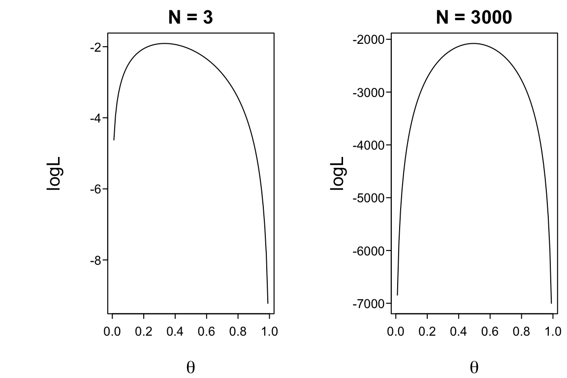
The information function is the expected value of the negative curvature in the log-likelihood: if the log-likelihood function has a distinct peak, we can easily discriminate between a good parameter estimate and a bad one.
Code
spar(mfrow=c(1,2), top=1)binom.loglik <-function(parms, y){ out <-dbinom(y, 1, parms, log=TRUE) sum(out)}p <-seq(0.01, 0.99, by =0.01)y1 <-rbinom(3, 1, 0.5)y2 <-rbinom(3000, 1, 0.5)ll1 <- ll2 <-numeric(length(p))for(i inseq_along(p)){ ll1[i] <-binom.loglik(p[i], y1) ll2[i] <-binom.loglik(p[i], y2)}plot(p, ll1, type ="l", ylab ="logL", xlab =expression(theta), main ="N = 3")plot(p, ll2, type ="l", ylab ="logL", xlab =expression(theta), main ="N = 3000")
Figure 9.1: Log-likelihood function for binomial distribution with 2 sample sizes
9.2 Review, continued
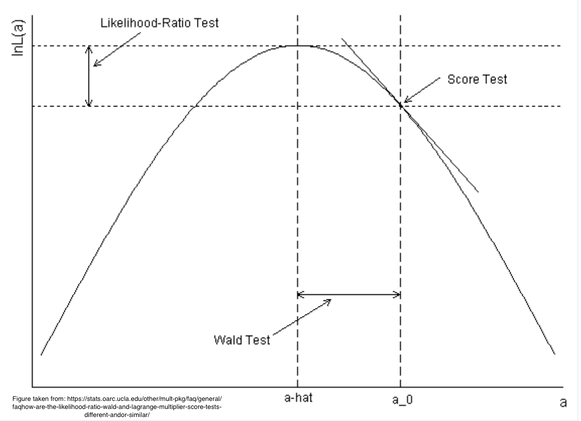
Likelihood Ratio Test (LR):
\[LR = -2\log(\text{L at } H_0/\text{L at MLE})\]
Wald Test (W):
\[W = \frac{(\hat{B} - B_0)^2}{Var(\hat{B})}\]
Score Test (S):
\[S = \frac{U(B_0)}{I(B_0)}\]
Figure 9.2: Tests arising from maximum liklihood estimation
9.3 Review, continued
The decision on which test to use is based on statistical and computational properties.
From the statistical point of view: LR is the best statistic followed by S and W. In logistic regression problems, W is sensitive to problems in the estimated variance-covariance matrix of the full model (see below)
From the computational point of view: Estimation of LR and W requires estimating all the unknown parameters. Additionally, estimation of LR requires two models.
9.4 The Hauck-Donner Effect
Especially for categorical regression models such as the binary and polytomous logistic models, problems arise when a part of the covariate space yields an outcome probability of zero or one so that there is perfect separation in a covariate distribution. Infinite regression coefficient estimates are fine, but Wald statistics become too small because as \(\hat{\beta} \rightarrow \infty\) the estimated standard error of \(\hat{\beta} \rightarrow \infty\) even faster. Here is a binary logistic model example where a binary predictor has a true coefficient of 25 which corresponds to an outcome probability within \(10^{-11}\) of 1.0.
The Wald \(\chi^2\) for x2 is 0.26 but the much better LR \(\chi^2\) is very large as one would expect from a variable having a large estimated coefficient. The standard error for the x2 log odds ratio blew up.
9.5 Confidence Intervals
What test should form the basis for the confidence interval?
The Wald test is the most frequently used.
The interval based on the Wald test is given by \(b_i \pm z_{1-\alpha/2}s\)
The Wald statistic might not always be good due to problems of the W in the estimation of the variance and covariance matrix
Wald-based statistics are convenient for deriving confidence intervals for linear or more complex combination of model’s parameters
LR and score-based confidence intervals also exist. However, they are computationally more intensive than the confidence interval based on the Wald statistic
Profile likelihood confidence intervals are probably best. See here for a nice example showing how to compute profile intervals on derived parameters.
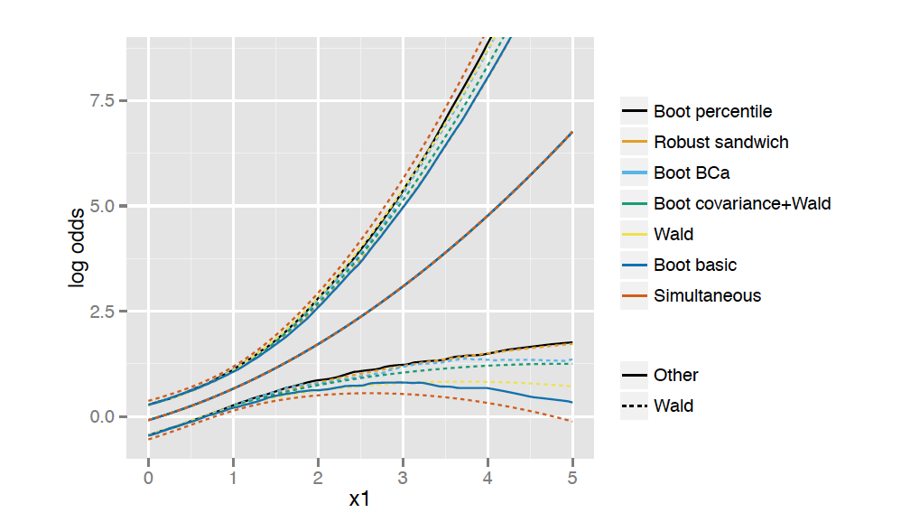
9.6 Boostrap Confidence Regions
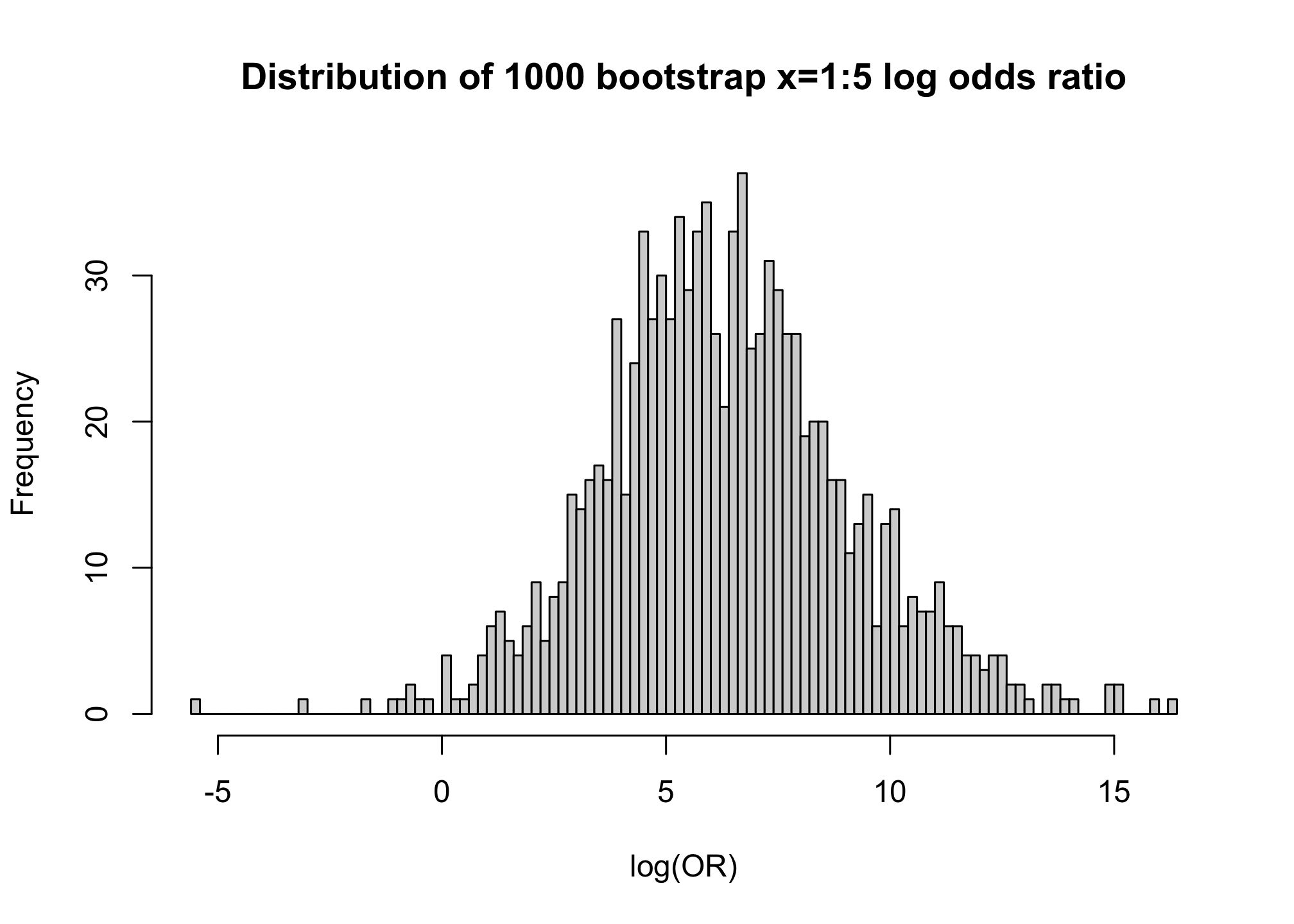
Confidence intervals for functions of the vector of parameters \(B\) can be computed using bootstrap percentile confidence limits.
from each sample with replacement of the original dataset compute the MLE of \(B\), \(b\).
compute the quantity of interest \(g(b)\)
sort \(g(b)\) and compute the desired percentiles
The method is suitable for obtaining pointwise confidence band for non linear functions
Other more complex bootstrap scheme exists
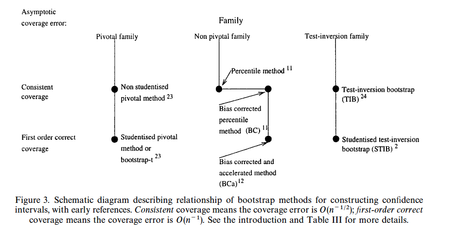
Carpenter & Bithell (2000) is an excellent article about bootstrap confidence intervals, describing when should we use them, which one should we pick, and how should we calculate the bootstrap confidence interval
The picture below is taken directly from the paper
Suppose we have data from one sample and we develop two models. The -2 log likelihood for models 1 and 2 are \(L_1\) and \(L_2\)
We observed \(L_1 < L_2\).
Which of the two models is the best?
–
Model 1 can provide a better fit for the data, but it might require a larger number of paramters
If model 1 is over fitting then it can results in worse results in a new dataset
AIC would choose the model by comparing \(L_1 + 2p_1\) with \(L_2 + 2p_2\) and selecting the model with the lowest value
Similar to AIC, BIC would select a model by accounting for the likelihood and the number of parameters
BIC would choose the model by comparing \(L_1 + p_1\log n\) with \(L_2 + p_2 \log n\) and selecting the model with the lowest value
Several authors have studied the AIC, BIC and other likelihood penalties. Some highlights:
AIC have “lower probability of correct model selection” in linear regression settings (Zheng & Loh, 1995)
“Our experience with large dataset in sociology is that the AIC selects models that are too big even when the sample size is large, including effects that are counterintuitive or not borne out by subsequent research”(Kass & Raftery, 1995)
There are cases where AIC yields consistent model selection but BIC does not (Kass & Raftery, 1995)
The corrected AIC improves AIC performance in small samples:
\[AIC_c = AIC + \frac{2p(p+1)}{n-p-1}\]
A very readable presentation about AIC and BIC by B. D. Ripley may be found here. Briefly, when the achieved log likelihood is evaluated in another sample of the same size, with parameter estimates set to the MLEs from the original sample, the expected value of the log-likelihood gets worse by the number of parameters estimated (if penalization is not used). Thus AIC represents an out-of-sample correction to the log likelihood, or an expected correction for overfitting.
Gelman, Hwang, and Vehtari have a very useful article here that places these issues in a Bayesian context.
9.8 Testing if model \(M_1\) is better than model \(M_2\)
To test if model \(M_1\) is better than model \(M_2\) we could:
combine \(M_1\) and \(M_2\) in a single model \(M_1\) + \(M_2\)
test whether \(M_1\) adds predictive information to \(M_2\)\((H_0: M_1+M_2>M_2)\)
test whether \(M_2\) adds predictive information to \(M_1\)\((H_0: M_1+M_2>M_1)\)
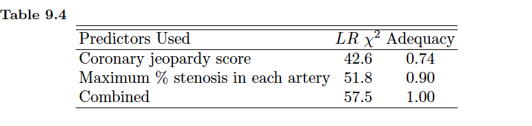
9.9 Unitless Index of Adequacy of a Subset of Predictors
\[A = \frac{LR^s}{LR}\]
\(LR^s\) is - 2 log-likelihood for testing the importance of the subset of predictors of interest (excluding the other predictors from the model).
\(LR\) is - 2 log-likelihood for testing the full model (i.e., the model with both sets of predictors)
\(A\) is the proportion of the log likelihood explained by the subset of predictors compared to the proportion of likelihood explained by the full set of predictors
When \(A = 0\), the subset does not have predictive information by itself
When \(A = 1\) the subset contains all the predictive information found in the whole set of predictors
9.10 Unitless Index of Predictive Ability
Best (lowest) possible \(-2LL\): \(L^* = -2LL\) for a hypothetical model that perfectly predicts the outcome
Achieved \(-2LL\): \(L = -2LL\) for the fitted model
Worst \(-2LL\): \(L^{0} = - 2LL\) for a model that has no predictive information
The fraction of \(-2LL\) explained that was capable of being explained is
Multiple authors have pointed out difficulties with the \(R^2\) in a logistic model. Different \(R^2\) measures have been provided. One of these measures is:
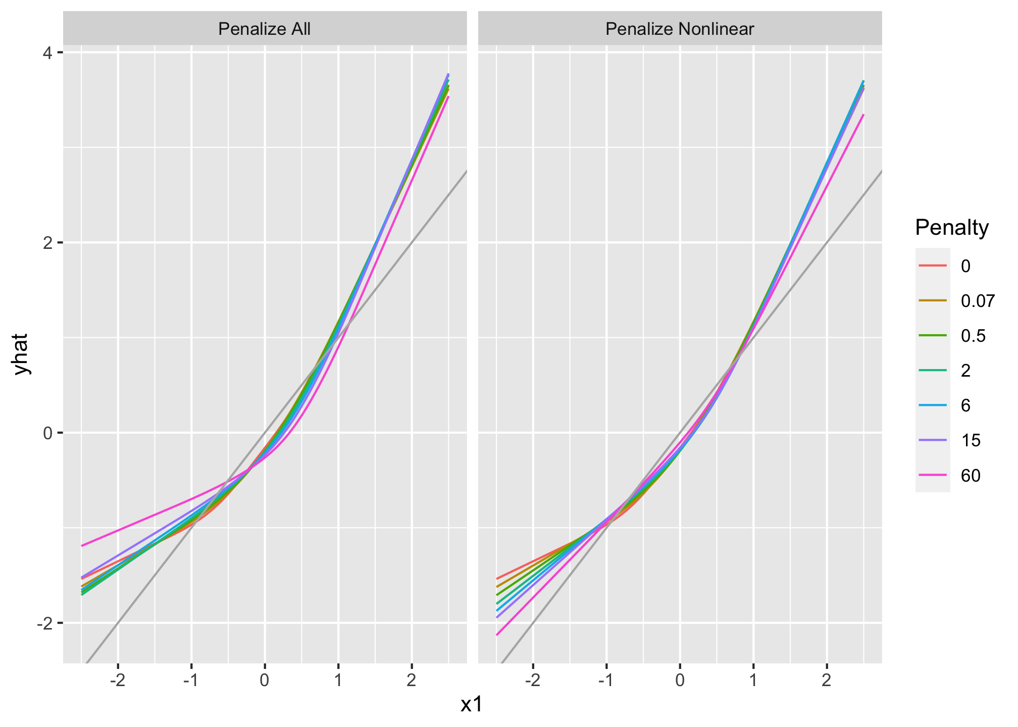
\[logL - \frac{1}{2}\lambda\sum_{i = 1}^p(s_i\beta_i)^2\] where \(s_i\) are scale factors chosen to make \(s_i\beta_i\) unitless.
Usual methods can be used to find \(\hat{\beta}^{P}\) that maximizes the log-likelihood. If we do not wish to shrink all the parameters we can set the scale constant to 0.
Choice of scaling \(s_i\). Most authors standardize the data first so they do not have the scale factors in their equation. A common choice is to use the standard deviation of each column of he design matrix. This choice is problematic for non linear term and for dummy variables.
For a categorical predictors with \(c\) levels the amount of shrinkage and the predicted values depend on which level was chosen as the reference. An alternative penalty function \(\sum_{i}(\beta_i-\bar{\beta})^2\) that shrinks the coefficient towards the mean has been proposed.
Effective number of parameters. Effective number of parameters changes for each \(\lambda\) due to shrinkage. The degrees of freedom can be calculated as:
Choosing \(\lambda\). To choose \(\lambda\) we can use the modified AIC
\[LR~ \chi^2 - 2\text{ effective d.f.}\]
where \(LR~ \chi^2\) is the likelihood ratio \(\chi^2\) for the penalized model, but ignoring the penalty function. The \(\lambda\) that maximizes the AIC will often be a good choice.
Describe in general terms why the information matrix is related to precision of MLEs.
Section 9.2
Explain in general terms how the Rao efficient score test works.
Section 9.3
For right-censored time-to-event data, what is the likelihood component for an uncensored and for a censored data value?
What makes the Wald test not very accurate in general?
Why are Wald confidence intervals symmetric?
Section 9.4
Why do we like the Newton-Raphson method for solving for MLEs?
Section 9.5
Why does the robust cluster sandwich covariance estimator not make sense at a fundamental level?
Will the cluster sandwich covariance estimator properly detect and ignore observations that are duplicated?
Section 9.7
Why are most bootstrap confidence intervals not extremely accurate (other than from the double bootstrap or the bootstrap t method)?
What is the real appeal of bootstrap confidence intervals?
Section 9.8
Why is AIC not an answer to the question of whether a biomarker is useful to know, after adjusting for other predictors?
What is the appeal of the adequacy index?
Section 9.10
What is are the main challenges with penalized MLE?
Can penalization hurt estimates?
What is the most principled method for doing statistical inference if one is penalizing parameter estimates?
Carpenter, J., & Bithell, J. (2000). Bootstrap confidence intervals: When, which, what? A practical guide for medical statisticians. Stat Med, 19, 1141–1164.
unconditional nonparametric bootstrap becomes more equivalent to conditional bootstrap based on regression residuals when full models are fitted
Harrell, F. E. (2015). Regression Modeling Strategies, with Applications to Linear Models, Logistic and Ordinal Regression, and Survival Analysis (Second edition). Springer. https://doi.org/10.1007/978-3-319-19425-7
Kass, R. E., & Raftery, A. E. (1995). Bayes factors. J Am Stat Assoc, 90, 773–795.
Zheng, X., & Loh, W.-L. (1995). Consistent variable selection in linear models. J Am Stat Assoc, 90, 151–156.
Source Code
```{r include=FALSE}require(rms)require(qreport)options(qproject='rms', prType='html')getRs('qbookfun.r')hookaddcap()knitr::set_alias(w = 'fig.width', h = 'fig.height', cap = 'fig.cap', scap ='fig.scap')```# Overview of Maximum Likelihood Estimation {#sec-mle}<center>Chiara Di Gravio<br>Department of Biostatistics<br>Vanderbilt University</center>## Review* References: @rms2, @kas95bay, @car00boo, @zhe95con* Maximum Likelihood estimation is a technique for estimating parameters and drawing statistical inferences $$L(B) = \prod_{i = 1}^n f_i(Y_i, B)$$* The first derivative of the log-likelihood function is the **score function $U(\theta)$** * The negative of the second derivative of the log-likelihood function is the **Fisher information**---* The information function is the expected value of the negative curvature in the log-likelihood: if the log-likelihood function has a distinct peak, we can easily discriminate between a good parameter estimate and a bad one.```{r, w=6, h=4}#| label: fig-mle-binomial#| fig-cap: "Log-likelihood function for binomial distribution with 2 sample sizes"spar(mfrow=c(1,2), top=1)binom.loglik <- function(parms, y){ out <- dbinom(y, 1, parms, log=TRUE) sum(out)}p <- seq(0.01, 0.99, by = 0.01)y1 <- rbinom(3, 1, 0.5)y2 <- rbinom(3000, 1, 0.5)ll1 <- ll2 <- numeric(length(p))for(i in seq_along(p)){ ll1[i] <- binom.loglik(p[i], y1) ll2[i] <- binom.loglik(p[i], y2)}plot(p, ll1, type = "l", ylab = "logL", xlab = expression(theta), main = "N = 3")plot(p, ll2, type = "l", ylab = "logL", xlab = expression(theta), main = "N = 3000")```---## Review, continuedLikelihood Ratio Test (LR): $$LR = -2\log(\text{L at } H_0/\text{L at MLE})$$Wald Test (W):$$W = \frac{(\hat{B} - B_0)^2}{Var(\hat{B})}$$Score Test (S):$$S = \frac{U(B_0)}{I(B_0)}$$```{r, out.width='100%', fig.align='center', echo=FALSE, fig.retina=3}#| label: fig-mle-liktest#| fig-cap: "Tests arising from maximum liklihood estimation"knitr::include_graphics('mle-liktest.png')```---## Review, continued* The decision on which test to use is based on statistical and computational properties.* From the **statistical point of view**: LR is the best statistic followed by S and W. In logistic regression problems, W is sensitive to problems in the estimated variance-covariance matrix of the full model (see below)* From the **computational point of view**: Estimation of LR and W requires estimating all the unknown parameters. Additionally, estimation of LR requires two models. ---## The Hauck-Donner Effect {#sec-mle-hd}Especially for categorical regression models such as the binary and polytomous logistic models, problems arise when a part of the covariate space yields an outcome probability of zero or one so that there is _perfect separation_ in a covariate distribution. Infinite regression coefficient estimates are fine, but Wald statistics become too small because as $\hat{\beta} \rightarrow \infty$ the estimated standard error of $\hat{\beta} \rightarrow \infty$ even faster. Here is a binary logistic model example where a binary predictor has a true coefficient of 25 which corresponds to an outcome probability within $10^{-11}$ of 1.0.```{r}set.seed(3)n <-200x1 <-sample(0:1, n, TRUE)x2 <-sample(0:1, n, TRUE)L <-0.4* x1 +25* x2y <-rbinom(n, 1, prob=plogis(L))f <-lrm(y ~ x1 + x2, x=TRUE, y=TRUE)fanova(f)anova(f, test='LR')```The Wald $\chi^2$ for `x2` is 0.26 but the much better LR $\chi^2$ is very large as one would expect from a variable having a large estimated coefficient. The standard error for the `x2` log odds ratio blew up.## Confidence Intervals {#sec-mle-ci}**What test should form the basis for the confidence interval?*** The Wald test is the most frequently used. + The interval based on the Wald test is given by $b_i \pm z_{1-\alpha/2}s$ + The Wald statistic might not always be good due to problems of the W in the estimation of the variance and covariance matrix + Wald-based statistics are convenient for deriving confidence intervals for linear or more complex combination of model's parameters* LR and score-based confidence intervals also exist. However, they are computationally more intensive than the confidence interval based on the Wald statistic* Profile likelihood confidence intervals are probably best. See [here](https://stats.stackexchange.com/a/588832/4253) for a nice example showing how to compute profile intervals on derived parameters.<!-- added 2022-09-16 -->---## Boostrap Confidence Regions {#sec-mle-boot}* Confidence intervals for functions of the vector of parameters $B$ can be computed using **bootstrap percentile** confidence limits. + from each sample with replacement of the original dataset compute the MLE of $B$, $b$. + compute the quantity of interest $g(b)$ + sort $g(b)$ and compute the desired percentiles* The method is suitable for obtaining pointwise confidence band for non linear functions* Other more complex bootstrap scheme exists---* @car00boo is an excellent article about bootstrap confidence intervals, describing when should we use them, which one should we pick, and how should we calculate the bootstrap confidence interval* The picture below is taken directly from the paper```{r, out.width='100%', fig.align='center', echo=FALSE, fig.retina=3}#| label: fig-mle-bootstrapEx#| fig-cap: "Bootstrap confidence interval choices, from @car00boo"knitr::include_graphics('mle-bootstrapEx.png')```---```{r}set.seed(15)n <-200x1 <-rnorm(n)logit <- x1 /2y <-ifelse(runif(n) <=plogis(logit), 1, 0)dd <-datadist(x1); options(datadist ="dd")f <-lrm(y ~pol(x1, 2), x =TRUE, y =TRUE)f```---```{r}X <-cbind(Intercept =1, predict(f, data.frame(x1 =c(1,5)), type ="x"))Xdif <- X[2,,drop=FALSE] - X[1,,drop=FALSE]Xdifb <-bootcov(f, B =1000)boot.log.odds.ratio <- b$boot.Coef %*%t(Xdif)sd(boot.log.odds.ratio)# summary() uses the bootstrap covariance matrixsummary(b, x1 =c(1,5))[1, "S.E."]```---```{r, w=7, fig.height=5, align = "center", fig.retina=3}contrast(b, list(x1 = 5), list(x1 = 1), fun = exp)hist(boot.log.odds.ratio, nclass = 100, xlab = "log(OR)", main = "Distribution of 1000 bootstrap x=1:5 log odds ratio")```---```{r}x1s <-seq(0, 5, length =100)pwald <-Predict(f, x1 = x1s) psand <-Predict(robcov(f), x1 = x1s) pbootcov <-Predict(b, x1 = x1s, usebootcoef =FALSE)pbootnp <-Predict(b, x1 = x1s) pbootbca <-Predict(b, x1 = x1s, boot.type ="bca") pbootbas <-Predict(b, x1 = x1s, boot.type ="basic")psimult <-Predict(b, x1 = x1s, conf.type ="simultaneous") ``````{r, out.width='100%', fig.align='center', echo=FALSE, fig.retina=3}#| label: fig-mle-bootci#| fig-cap: "Bootstrap confidence intervals"knitr::include_graphics('mle-bootCi.png')```---## AIC & BIC {#sec-mle-aic}* Suppose we have data from one sample and we develop two models. The -2 log likelihood for models 1 and 2 are $L_1$ and $L_2$* We observed $L_1 < L_2$. * Which of the two models is the best?--* Model 1 can provide a better fit for the data, but it might require a larger number of paramters* If model 1 is over fitting then it can results in worse results in a new dataset---* AIC would choose the model by comparing $L_1 + 2p_1$ with $L_2 + 2p_2$ and selecting the model with the lowest value* Similar to AIC, BIC would select a model by accounting for the likelihood and the number of parameters* BIC would choose the model by comparing $L_1 + p_1\log n$ with $L_2 + p_2 \log n$ and selecting the model with the lowest value* Several authors have studied the AIC, BIC and other likelihood penalties. Some highlights: + AIC have _"lower probability of correct model selection"_ in linear regression settings [@zhe95con] + *"Our experience with large dataset in sociology is that the AIC selects models that are too big even when the sample size is large, including effects that are counterintuitive or not borne out by subsequent research"* [@kas95bay] + There are cases where AIC yields consistent model selection but BIC does not [@kas95bay]* The corrected AIC improves AIC performance in small samples:$$AIC_c = AIC + \frac{2p(p+1)}{n-p-1}$$A very readable presentation about AIC and BIC by B. D. Ripley may be found [here](https://www.stats.ox.ac.uk/~ripley/Nelder80.pdf). Briefly, when the achieved log likelihood is evaluated in another sample of the same size, with parameter estimates set to the MLEs from the original sample, the expected value of the log-likelihood gets worse by the number of parameters estimated (if penalization is not used). Thus AIC represents an out-of-sample correction to the log likelihood, or an expected correction for overfitting.Gelman, Hwang, and Vehtari have a very useful article [here](http://www.stat.columbia.edu/~gelman/research/published/waic_understand3.pdf) that places these issues in a Bayesian context.----## Testing if model $M_1$ is better than model $M_2$* To test if model $M_1$ is better than model $M_2$ we could: + combine $M_1$ and $M_2$ in a single model $M_1$ + $M_2$ + test whether $M_1$ adds predictive information to $M_2$ $(H_0: M_1+M_2>M_2)$ * test whether $M_2$ adds predictive information to $M_1$ $(H_0: M_1+M_2>M_1)$```{r, out.width='100%', fig.align='center', echo=FALSE, fig.retina=3}knitr::include_graphics('mle-table.png')```----## Unitless Index of Adequacy of a Subset of Predictors$$A = \frac{LR^s}{LR}$$* $LR^s$ is - 2 log-likelihood for testing the importance of the subset of predictors of interest (excluding the other predictors from the model).* $LR$ is - 2 log-likelihood for testing the full model (i.e., the model with both sets of predictors)* $A$ is the proportion of the log likelihood explained by the subset of predictors compared to the proportion of likelihood explained by the full set of predictors---* When $A = 0$, the subset does not have predictive information by itself* When $A = 1$ the subset contains all the predictive information found in the whole set of predictors---## Unitless Index of Predictive Ability1. Best (lowest) possible $-2LL$: $L^* = -2LL$ for a hypothetical model that perfectly predicts the outcome2. Achieved $-2LL$: $L = -2LL$ for the fitted model3. Worst $-2LL$: $L^{0} = - 2LL$ for a model that has no predictive information* The fraction of $-2LL$ explained that was capable of being explained is$$\frac{L^{0} - L}{L^{0} - L^{*}} = \frac{LR}{L^{0}-L^{*}}$$* We can penalise this measure by accounting for the number of parameters $p$:$$R^{2} = \frac{LR - 2p}{L^{0}-L^{*}}$$---* A partial $R^2$ index can also be defined where we consider the amount of likelihood explained by a single factor instead of the full model$$R_{partial}^{2} = \frac{LR_{partial} - 2}{L^{0}-L^{*}}$$* Multiple authors have pointed out difficulties with the $R^2$ in a logistic model. Different $R^2$ measures have been provided. One of these measures is:$$R^{2}_{LR} = 1 - \exp(LR/n) = 1 - \lambda^{2/n}$$where $\lambda$ is the null model likelihood divided by the fitted model likelihood* Cragg, Uhler and Nagelkerke suggested dividing $R^{2}_{LR}$ by its maximum attainable value to derive a measure ranging from 0 to 1:$$R^{2}_{N} = \frac{1 - \exp(LR/n)}{1-\exp(L^0/n)}$$----## Penalized Maximum Likelihood {#sec-mle-pmle}* A general formula for penalized likelihood;$$logL - \frac{1}{2}\lambda\sum_{i = 1}^p(s_i\beta_i)^2$$ where $s_i$ are scale factors chosen to make $s_i\beta_i$ unitless.* Usual methods can be used to find $\hat{\beta}^{P}$ that maximizes the log-likelihood. If we do not wish to shrink all the parameters we can set the scale constant to 0.* **Choice of scaling $s_i$.** Most authors standardize the data first so they do not have the scale factors in their equation. A common choice is to use the standard deviation of each column of he design matrix. This choice is problematic for non linear term and for dummy variables.* For a categorical predictors with $c$ levels the amount of shrinkage and the predicted values depend on which level was chosen as the reference. An alternative penalty function $\sum_{i}(\beta_i-\bar{\beta})^2$ that shrinks the coefficient towards the mean has been proposed.---**Effective number of parameters.** Effective number of parameters changes for each $\lambda$ due to shrinkage. The degrees of freedom can be calculated as:$$\mathrm{trace}\left[I\left(\hat{\beta}^P\right)V\left(\hat{\beta}^P\right)\right]$$**Choosing $\lambda$.** To choose $\lambda$ we can use the modified AIC$$LR~ \chi^2 - 2\text{ effective d.f.}$$where $LR~ \chi^2$ is the likelihood ratio $\chi^2$ for the penalized model, but ignoring the penalty function. The $\lambda$ that maximizes the AIC will often be a good choice.---```{r}set.seed(191)x1 <-rnorm (100)y <- x1 +rnorm (100)pens <- df <- aic <-c(0, 0.07, 0.5, 2, 6, 15, 60)all <- nl <-list()df.tot <-NULLfor(penalize in1:2){for(i in1:length(pens)){ f <-ols(y ~rcs(x1, 5), penalty =list(simple =if(penalize==1)pens[i] else0 ,nonlinear = pens[i])) df[i] <- f$stat["d.f."] aic[i] <-AIC(f) nam <-paste(if(penalize ==1) "all"else"nl", "penalty:", pens[i], sep="") nam <-as.character(pens[i]) p <-Predict(f, x1 =seq(-2.5, 2.5, length =100), conf.int =FALSE)if(penalize ==1) all[[nam]] <- p else nl[[nam]] <- p } df.tot <-rbind(df.tot, rbind(df=df, aic=aic))}```---```{r, echo = FALSE, fig.align='center', fig.retina=3}knitr::kable(df.tot)all <- do.call(rbind, all); all$type <- "Penalize All"nl <- do.call(rbind, nl); nl$type <- "Penalize Nonlinear"both <- as.data.frame(rbind.data.frame(all, nl))both$Penalty <- both$.set.ggplot(both, aes(x=x1, y=yhat, color=Penalty)) + geom_line() + geom_abline(col=gray(0.7)) + facet_grid (~ type)```## Further Reading* [Quadratic approximation and normal asymptotics](https://strimmerlab.github.io/publications/lecture-notes/MATH20802/quadratic-approximation-and-normal-asymptotics.html) by Korbinian Strimmer## Study Questions**Section 9.1**1. What does the MLE optimize?1. Describe in general terms why the information matrix is related to precision of MLEs.**Section 9.2**1. Explain in general terms how the Rao efficient score test works.**Section 9.3**1. For right-censored time-to-event data, what is the likelihood component for an uncensored and for a censored data value?1. What makes the Wald test not very accurate in general?1. Why are Wald confidence intervals symmetric?**Section 9.4**1. Why do we like the Newton-Raphson method for solving for MLEs?**Section 9.5**1. Why does the robust cluster sandwich covariance estimator not make sense at a fundamental level?1. Will the cluster sandwich covariance estimator properly detect and ignore observations that are duplicated?**Section 9.7**1. Why are most bootstrap confidence intervals not extremely accurate (other than from the double bootstrap or the bootstrap t method)?1. What is the real appeal of bootstrap confidence intervals?**Section 9.8**1. Why is AIC not an answer to the question of whether a biomarker is useful to know, after adjusting for other predictors?1. What is the appeal of the adequacy index?**Section 9.10**1. What is are the main challenges with penalized MLE?1. Can penalization hurt estimates?1. What is the most principled method for doing statistical inference if one is penalizing parameter estimates?```{r echo=FALSE}saveCap('09')```