4  Multivariable Modeling Strategies

• “Spending d.f.”: examining or fitting parameters in models, or examining tables or graphs that utilize \(Y\) to tell you how to model variables
• If wish to preserve statistical properties, can’t retrieve d.f. once they are “spent” (see Grambsch & O’Brien)
• If a scatterplot suggests linearity and you fit a linear model, how many d.f. did you actually spend (i.e., the d.f. that when put into a formula results in accurate confidence limits or \(P\)-values)?
• Decide number of d.f. that can be spent
• Decide where to spend them
• Spend them
• General references: (Giudice et al., 2011; Frank E. Harrell et al., 1996; Nick & Hardin, 1999; Steyerberg et al., 2001)

AB

There are many choices to be made when deciding upon a global modeling strategy, including choice between

• parametric and nonparametric procedures
• parsimony and complexity
• parsimony and good discrimination ability
• interpretable models and black boxes.

C

4.1 Prespecification of Predictor Complexity Without Later Simplification

• Rarely expect linearity
• Can’t always use graphs or other devices to choose transformation
• If select from among many transformations, results biased
• Need to allow flexible nonlinearity to potentially strong predictors not known to predict linearly
• Once decide a predictor is “in” can choose no. of parameters to devote to it using a general association index with \(Y\)
• Need a measure of “potential predictive punch”
• Measure needs to mask analyst to true form of regression to preserve statistical properties

D

Motivating examples:

# Overfitting a flat relationship
require(rms)
set.seed(1)
x <- runif(1000)
y <- runif(1000, -0.5, 0.5)
dd <- datadist(x, y); options(datadist='dd')
par(mfrow=c(2,2), mar=c(2, 2, 3, 0.5))
pp <- function(actual) {
  yhat  <- predict(f, data.frame(x=xs))
  yreal <- actual(xs)
  plot(0, 0, xlim=c(0,1),
       ylim=range(c(quantile(y, c(0.1, 0.9)), yhat,
                    yreal)),
       type='n', axes=FALSE)
  axis(1, labels=FALSE); axis(2, labels=FALSE)
  lines(xs, yreal)
  lines(xs, yhat, col='blue')
}
f <- ols(y ~ rcs(x, 5))
xs <- seq(0, 1, length=150)
pp(function(x) 0*x)
title('Mild Error:\nOverfitting a Flat Relationship',
      cex=0.5)
y <- x + runif(1000, -0.5, 0.5)
f <- ols(y ~ rcs(x, 5))
pp(function(x) x)
title('Mild Error:\nOverfitting a Linear Relationship',
      cex=0.5)
y <- x^4 + runif(1000, -1, 1)
f <- ols(y ~ x)
pp(function(x) x^4)
title('Serious Error:\nUnderfitting a Steep Relationship',
      cex=0.5)
y <- - (x - 0.5) ^ 2 + runif(1000, -0.2, 0.2)
f <- ols(y ~ x)
pp(function(x) - (x - 0.5) ^ 2)
title('Tragic Error:\nMonotonic Fit to\nNon-Monotonic Relationship',
      cex=0.5)

Figure 4.1: Fitting errors to withstand or to avoid

Examples of Reducing the Number of Parameters

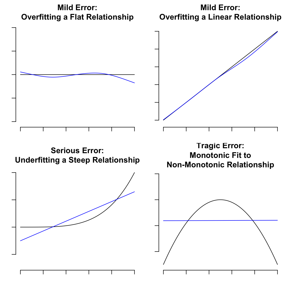
Categorical predictor with \(k\) levels	Collapse less frequent categories into “other”
Continuous predictor represented as \(k\)-knot restricted cubic spline	Reduce \(k\) to a number as low as 3, or 0 (linear)

E

4.1.1 Learning From a Saturated Model

When the effective sample size available is sufficiently large so that a saturated main effects model may be fitted, a good approach to gauging predictive potential is the following.

• Let all continuous predictors be represented as restricted cubic splines with \(k\) knots, where \(k\) is the maximum number of knots the analyst entertains for the current problem.
• Let all categorical predictors retain their original categories except for pooling of very low prevalence categories (e.g., ones containing \(<6\) observations).
• Fit this general main effects model.
• Compute the partial \(\chi^2\) statistic for testing the association of each predictor with the response, adjusted for all other predictors. In the case of ordinary regression convert partial \(F\) statistics to \(\chi^2\) statistics or partial \(R^2\) values.
• Make corrections for chance associations to “level the playing field” for predictors having greatly varying d.f., e.g., subtract the d.f. from the partial \(\chi^2\) (the expected value of \(\chi^{2}_{p}\) is \(p\) under \(H_{0}\)).
• Make certain that tests of nonlinearity are not revealed as this would bias the analyst.
• Sort the partial association statistics in descending order.

F

Commands in the rms package can be used to plot only what is needed. Here is an example for a logistic model.

f <- lrm(y ~ sex + race + rcs(age,5) + rcs(weight,5) +
         rcs(height,5) + rcs(blood.pressure,5))
plot(anova(f))

4.1.2 Using Marginal Generalized Rank Correlations

When collinearities or confounding are not problematic, a quicker approach based on pairwise measures of association can be useful. This approach will not have numerical problems (e.g., singular covariance matrix) and is based on:

• 2 d.f. generalization of Spearman \(\rho\)—\(R^2\) based on \(rank(X)\) and \(rank(X)^2\) vs. \(rank(Y)\)
• \(\rho^2\) can detect U-shaped relationships
• For categorical \(X\), \(\rho^2\) is \(R^2\) from dummy variables regressed against \(rank(Y)\); this is tightly related to the Wilcoxon-Mann-Whitney-Kruskal-Wallis rank test for group differences¹
• Sort variables by descending order of \(\rho^2\)
• Specify number of knots for continuous \(X\), combine infrequent categories of categorical \(X\) based on \(\rho^2\)

G

¹ This test statistic does not inform the analyst of which groups are different from one another.

Allocating d.f. based on partial tests of association or sorting \(\rho^2\) is a fair procedure because

• We already decided to keep variable in model no matter what \(\rho^2\) or \(\chi^2\) values are seen
• \(\rho^2\) and \(\chi^2\) do not reveal degree of nonlinearity; high value may be due solely to strong linear effect
• low \(\rho^2\) or \(\chi^2\) for a categorical variable might lead to collapsing the most disparate categories

H

Initial simulations show the procedure to be conservative. Note that one can move from simpler to more complex models but not the other way round

4.2 Checking Assumptions of Multiple Predictors Simultaneously

• Sometimes failure to adjust for other variables gives wrong transformation of an \(X\), or wrong significance of interactions
• Sometimes unwieldy to deal simultaneously with all predictors at each stage \(\rightarrow\) assess regression assumptions separately for each predictor

I

4.3 Variable Selection

• Series of potential predictors with no prior knowledge
• \(\uparrow\) exploration \(\rightarrow\) \(\uparrow\) shrinkage (overfitting)
• Summary of problem: \(E(\hat{\beta} | \hat{\beta}\) “significant” \() \neq \beta\) (Chatfield, 1995)
• Biased \(R^2\), \(\hat{\beta}\), standard errors, \(P\)-values too small
• \(F\) and \(\chi^2\) statistics do not have the claimed distribution² (Grambsch & O’Brien, 1991)
• Will result in residual confounding if use variable selection to find confounders (Greenland, 2000)
• Derksen & Keselman (1992) found that in stepwise analyses the final model represented noise 0.20-0.74 of time, final model usually contained \(< \frac{1}{2}\) actual number of authentic predictors. Also:

J

² Lockhart et al. (2013) provide an example with \(n=100\) and 10 orthogonal predictors where all true \(\beta\)s are zero. The test statistic for the first variable to enter has type I assertion probability of 0.39 when the nominal \(\alpha\) is set to 0.05.

K

1. The degree of correlation between the predictor variables affected the frequency with which authentic predictor variables found their way into the final model.
2. The number of candidate predictor variables affected the number of noise variables that gained entry to the model.
3. The size of the sample was of little practical importance in determining the number of authentic variables contained in the final model.
4. The population multiple coefficient of determination could be faithfully estimated by adopting a statistic that is adjusted by the total number of candidate predictor variables rather than the number of variables in the final model.

• Global test with \(p\) d.f. insignificant \(\rightarrow\) stop

Simulation experiment, true \(\sigma^{2} = 6.25\), 8 candidate variables, 4 of them related to \(Y\) in the population. Select best model using all possible subsets regression to maximize \(R^{2}_{adj}\) (all possible subsets is not usually recommended but gives variable selection more of a chance to work in this context).

L

Note: The audio was made using stepAIC with collinearities in predictors. The code below allows for several options. Here we use all possible subsets of predictors and force predictors to be uncorrelated, which is the easiest case for variable selection.

require(MASS)    # provides stepAIC function
require(leaps)   # provides regsubsets function
sim <- function(n, sigma=2.5, method=c('stepaic', 'leaps'),
                pr=FALSE, prcor=FALSE, dataonly=FALSE) {
  method <- match.arg(method)
  if(uncorrelated) {
    x1 <- rnorm(n)
    x2 <- rnorm(n)
    x3 <- rnorm(n)
    x4 <- rnorm(n)
    x5 <- rnorm(n)
    x6 <- rnorm(n)
    x7 <- rnorm(n)
    x8 <- rnorm(n)
    }
  else {
      x1 <- rnorm(n)
      x2 <- x1 + 2.0 * rnorm(n)       # was + 0.5 * rnorm(n)
      x3 <- rnorm(n)
      x4 <- x3 + 1.5 * rnorm(n)
      x5 <- x1 + rnorm(n)/1.3
      x6 <- x2 + 2.25 * rnorm(n)      # was rnorm(n)/1.3
      x7 <- x3 + x4 + 2.5 * rnorm(n)  # was + rnorm(n)
      x8 <- x7 + 4.0 * rnorm(n)       # was + 0.5 * rnorm(n)
  }
  z <- cbind(x1,x2,x3,x4,x5,x6,x7,x8)
  if(prcor) return(round(cor(z), 2))
  lp <- x1 + x2 + .5*x3 + .4*x7
  y <- lp + sigma*rnorm(n)
  if(dataonly) return(list(x=z, y=y))
  if(method == 'leaps') {
    s     <- summary(regsubsets(z, y))
    best  <- which.max(s$adjr2)
    xvars <- s$which[best, -1]   # remove intercept
    ssr   <- s$rss[best]
    p     <- sum(xvars)
    xs    <- if(p == 0) 'none' else paste((1 : 8)[xvars], collapse='')
    if(pr) print(xs)
    ssesw <- (n - 1) * var(y) - ssr
    s2s   <- ssesw / (n - p - 1)
    yhat  <- if(p == 0) mean(y) else fitted(lm(y ~ z[, xvars]))
  }
  f <- lm(y ~ x1 + x2 + x3 + x4 + x5 + x6 + x7 + x8)
  if(method == 'stepaic') {
    g <- stepAIC(f, trace=0)
    p <- g$rank - 1
    xs <- if(p == 0) 'none' else
      gsub('[ <br>+x]','', as.character(formula(g))[3])
    if(pr) print(formula(g), showEnv=FALSE)
    ssesw <- sum(resid(g)^2)
    s2s   <- ssesw/g$df.residual
    yhat  <- fitted(g)
  }
  # Set SSEsw / (n - gdf - 1) = true sigma^2
  gdf <- n - 1 - ssesw / (sigma^2)
  # Compute root mean squared error against true linear predictor
  rmse.full <- sqrt(mean((fitted(f) - lp) ^ 2))
  rmse.step <- sqrt(mean((yhat - lp) ^ 2))
  list(stats=c(n=n, vratio=s2s/(sigma^2),
         gdf=gdf, apparentdf=p, rmse.full=rmse.full, rmse.step=rmse.step),
       xselected=xs)
}

rsim <- function(B, n, method=c('stepaic', 'leaps')) {
  method <- match.arg(method)
  xs <- character(B)
  r <- matrix(NA, nrow=B, ncol=6)
  for(i in 1:B) {
    w     <- sim(n, method=method)
    r[i,] <- w$stats
    xs[i] <- w$xselected
  }
  colnames(r) <- names(w$stats)
  s <- apply(r, 2, median)
  p <- r[, 'apparentdf']
  s['apparentdf'] <- mean(p)
  print(round(s, 2))
  print(table(p))
  cat('Prob[correct model]=', round(sum(xs == '1237')/B, 2), '\n')
}

Show the correlation matrix being assumed for the \(X\)s:

uncorrelated <- TRUE
sim(50000, prcor=TRUE)

      x1   x2    x3   x4   x5   x6   x7    x8
x1  1.00 0.00 -0.01 0.00 0.01 0.01 0.00  0.01
x2  0.00 1.00  0.00 0.00 0.01 0.00 0.00  0.00
x3 -0.01 0.00  1.00 0.00 0.00 0.00 0.00 -0.01
x4  0.00 0.00  0.00 1.00 0.01 0.00 0.00  0.01
x5  0.01 0.01  0.00 0.01 1.00 0.01 0.00  0.00
x6  0.01 0.00  0.00 0.00 0.01 1.00 0.00  0.00
x7  0.00 0.00  0.00 0.00 0.00 0.00 1.00  0.01
x8  0.01 0.00 -0.01 0.01 0.00 0.00 0.01  1.00

Simulate to find the distribution of the number of variables selected, the proportion of simulations in which the true model (\(X_{1}, X_{2}, X_{3}, X_{7}\)) was found, the median value of \(\hat{\sigma}^{2}/\sigma^{2}\), the median effective d.f., and the mean number of apparent d.f., for varying sample sizes.

M

set.seed(11)
m <- 'leaps'             # all possible regressions stopping on R2adj
rsim(100, 20, method=m)  # actual model found twice out of 100

         n     vratio        gdf apparentdf  rmse.full  rmse.step 
     20.00       0.94       5.32       4.10       1.62       1.58 
p
 1  2  3  4  5  6  7  8 
 3 14 18 22 27 11  4  1 
Prob[correct model]= 0.02 

rsim(100, 40, method=m)

         n     vratio        gdf apparentdf  rmse.full  rmse.step 
     40.00       0.61      17.89       4.38       1.21       1.24 
p
 2  3  4  5  6  7 
 9 18 24 29 15  5 
Prob[correct model]= 0.04 

rsim(100, 150, method=m)

         n     vratio        gdf apparentdf  rmse.full  rmse.step 
    150.00       0.44      85.99       5.01       0.59       0.57 
p
 2  3  4  5  6  7  8 
 1  5 27 35 24  7  1 
Prob[correct model]= 0.2 

rsim(100, 300, method=m)

         n     vratio        gdf apparentdf  rmse.full  rmse.step 
    300.00       0.42     177.01       5.16       0.43       0.40 
p
 4  5  6  7  8 
27 42 20 10  1 
Prob[correct model]= 0.26 

rsim(100, 2000)

         n     vratio        gdf apparentdf  rmse.full  rmse.step 
   2000.00       1.00       6.43       4.58       0.17       0.15 
p
 4  5  6  7 
53 37  9  1 
Prob[correct model]= 0.53 

As \(n\uparrow\) the mean number of variables selected increased. The proportion of simulations in which the correct model was found increased from 0 to 0.53. \(\sigma^{2}\) is underestimated when \(n=300\) by a factor of 0.42, resulting in the d.f. needed to de-bias \(\hat{\sigma^{2}}\) being greater than \(n\) when the apparent d.f. was only 5.16 on the average. Variable selection slightly increased closeness to the true \(X\beta\).

If the simulations are re-run allowing for collinearities (uncorrelated=FALSE) one can expect variable selection to be even more problematic.

Variable selection methods (F. E. Harrell, 1986):

• Forward selection, backward elimination
• Stopping rule: “residual \(\chi^{2}\)” with d.f. = no. candidates remaining at current step
• Test for significance or use Akaike’s information criterion (AIC (Atkinson, 1980)), here \(\chi^{2}-2 \times d.f.\)
• Better to use subject matter knowledge!
• No currently available stopping rule was developed for stepwise, only for comparing a limited number of pre-specified models(Leo Breiman, 1992, sec. 1.3)
• Roecker (1991) studied forward selection (FS), all possible subsets selection (APS), full fits
• APS more likely to select smaller, less accurate models than FS
• Neither as accurate as full model fit unless more than half of candidate variables redundant or unnecessary
• Step-down is usually better than forward (Mantel, 1970) and can be used efficiently with maximum likelihood estimation (Lawless & Singhal, 1978)
• Fruitless to try different stepwise methods to look for agreement (Wiegand, 2010)
• Bootstrap can help decide between full and reduced model
• Full model fits gives meaningful confidence intervals with standard formulas, C.I. after stepwise does not (Altman & Andersen, 1989; Leo Breiman, 1992; Hurvich & Tsai, 1990)
• Data reduction (grouping variables) can help
• Using the bootstrap to select important variables for inclusion in the final model (Sauerbrei & Schumacher, 1992) is problematic (Austin, 2008)
• It is not logical that a population regression coefficient would be exactly zero just because its estimate was “insignificant”

NOP

See also these articles:

• Step away from stepwise by Gary Smith
• Five myths about variable selection by Georg Heinze and Daniela Dunkler
• Variable selection - A review and recommendations for the practicing statistician by Georg Heinze, Christine Wallisch, Daniela Dunkler
• Stopping stepwise by Peter Flom

Q

4.3.1 Maxwell’s Demon as an Analogy to Variable Selection

Some of the information in the data is spent on variable selection instead of using all information for estimation.

Model specification is preferred to model selection.

Information content of the data usually insufficient for reliable variable selection.

James Clerk Maxwell

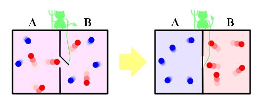
Maxwell imagines one container divided into two parts, A and B. Both parts are filled with the same gas at equal temperatures and placed next to each other. Observing the molecules on both sides, an imaginary demon guards a trapdoor between the two parts. When a faster-than-average molecule from A flies towards the trapdoor, the demon opens it, and the molecule will fly from A to B. Likewise, when a slower-than-average molecule from B flies towards the trapdoor, the demon will let it pass from B to A. The average speed of the molecules in B will have increased while in A they will have slowed down on average. Since average molecular speed corresponds to temperature, the temperature decreases in A and increases in B, contrary to the second law of thermodynamics.

Szilárd pointed out that a real-life Maxwell’s demon would need to have some means of measuring molecular speed, and that the act of acquiring information would require an expenditure of energy. Since the demon and the gas are interacting, we must consider the total entropy of the gas and the demon combined. The expenditure of energy by the demon will cause an increase in the entropy of the demon, which will be larger than the lowering of the entropy of the gas.

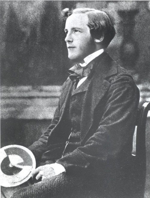
Source: commons.wikimedia.org/wiki/File:YoungJamesClerkMaxwell.jpg
en.wikipedia.org/wiki/Maxwell’s_demon

Peter Ellis’ blog article contains excellent examples of issues discussed here but applied to time series modeling.

4.4 Overfitting and Limits on Number of Predictors

• Concerned with avoiding overfitting
• Assume typical problem in medicine, epidemiology, and the social sciences in which the signal:noise ratio is small (higher ratios allow for more aggressive modeling)
• \(p\) should be \(< \frac{m}{15}\) (F. E. Harrell et al., 1984, 1985; Peduzzi et al., 1995, 1996; Smith et al., 1992; van der Ploeg et al., 2014; Vittinghoff & McCulloch, 2006)
• \(p\) is number of parameters in full model or number of candidate parameters in a stepwise analysis
• Derived from simulations to find minimum sample size so that apparent discrimination = validated discrimination
• Applies to typical signal:noise ratios found outside of tightly controlled experiments
• If true \(R^{2}\) is high, many parameters can be estimated from smaller samples
• Ignores sample size needed just to estimate the intercept or, in semiparametric models, the underlying distribution function³
• Riley, Snell, Ensor, Burke, Jr, et al. (2019) and Riley, Snell, Ensor, Burke, Harrell, et al. (2019) have refined sample size estimation for continuous, binary, and time-to-event models to account for all of these issues
• To just estimate \(\sigma\) in a linear model with a multiplicative margin of error of 1.2 with 0.95 confidence requires \(n=70\)

R

³ The sample size needed for these is model-dependent

S

Limiting Sample Sizes for Various Response Variable Types

Type of Response Variable	Limiting Sample Size \(m\)
Continuous	\(n\) (total sample size)
Binary	\(3np(1-p), p=\frac{n_{2}}{n}\) 4
Ordinal (\(k\) categories)	\(n - \frac{1}{n^{2}} \sum_{i=1}^{k} n_{i}^{3}\) 5
Failure (survival) time	number of failures 6

⁴ If one considers the power of a two-sample binomial test compared with a Wilcoxon test if the response could be made continuous and the proportional odds assumption holds, the effective sample size for a binary response is \(3 n_{1}n_{2}/n \approx 3 \min(n_{1}, n_{2})\) if \(\frac{n_{1}}{n}\) is near 0 or 1 (Whitehead, 1993, Eq. 10, 15). Here \(n_{1}\) and \(n_{2}\) are the marginal frequencies of the two response levels (Peduzzi et al., 1996). The effective sample size is a maximum (\(0.75n\)) when \(n_{1}=n_{2}\), i.e. \(p=\frac{1}{2}\) .

⁵ Based on the power of a proportional odds model two-sample test when the marginal cell sizes for the response are \(n_{1}, \ldots, n_{k}\), compared with all cell sizes equal to unity (response is continuous) (Whitehead, 1993, Eq. 3). If all cell sizes are equal, the relative efficiency of having \(k\) response categories compared to a continuous response is \(1 - \frac{1}{k^{2}}\) (Whitehead, 1993, Eq. 14), e.g., a 5-level response is almost as efficient as a continuous one if proportional odds holds across category cutoffs.

⁶ This is approximate, as the effective sample size may sometimes be boosted somewhat by censored observations, especially for non-proportional hazards methods such as Wilcoxon-type tests (Benedetti et al., 1982).

• Narrowly distributed predictor \(\rightarrow\) even higher \(n\)
• \(p\) includes all variables screened for association with response, including interactions
• Univariable screening (graphs, crosstabs, etc.) in no way reduces multiple comparison problems of model building (Sun et al., 1996)

T

More About the Binary \(Y\) Case

To derive the effective sample size for binary \(Y\) we compare two samples of equal size \(\frac{n}{2}\) by testing whether the log odds ratio is zero. When the two samples come from populations with equal \(\Pr(Y=1) = p\), the variance of the log odds ratio is approximately \(2 \times \frac{1}{\frac{n}{2}p(1-p)} = \frac{4}{np(1-p)}\). When \(Y\) is continuous with no ties and a Wilcoxon or proportional odds model test is used, the reciprocal of the variance of the proportional odds model’s log odds ratio is \(\frac{n^{3}}{12 (n+1)^{2}} \times (1 - \frac{1}{n^{2}}) \approx \frac{n}{12}\) so the variance is approximately \(\frac{12}{n}\). The ratio of this to the binary \(Y\) variance is \(3p(1-p)\).

4.5 Shrinkage

• Slope of calibration plot; regression to the mean
• Statistical estimation procedure — “pre-shrunk” models
• Aren’t regression coefficients OK because they’re unbiased?
• Problem is in how we use coefficient estimates
• Consider 20 samples of size \(n=50\) from \(U(0,1)\)
• Compute group means and plot in ascending order
• Equivalent to fitting an intercept and 19 dummies using least squares
• Result generalizes to general problems in plotting \(Y\) vs.
  \(X\hat{\beta}\)

U

set.seed(123)
n <- 50
y <- runif(20*n)
group <- rep(1:20,each=n)
ybar <- tapply(y, group, mean)
ybar <- sort(ybar)
plot(1:20, ybar, type='n', axes=FALSE, ylim=c(.3,.7),
     xlab='Group', ylab='Group Mean')
lines(1:20, ybar)
points(1:20, ybar, pch=20, cex=.5)
axis(2)
axis(1, at=1:20, labels=FALSE)
for(j in 1:20) axis(1, at=j, labels=names(ybar)[j])

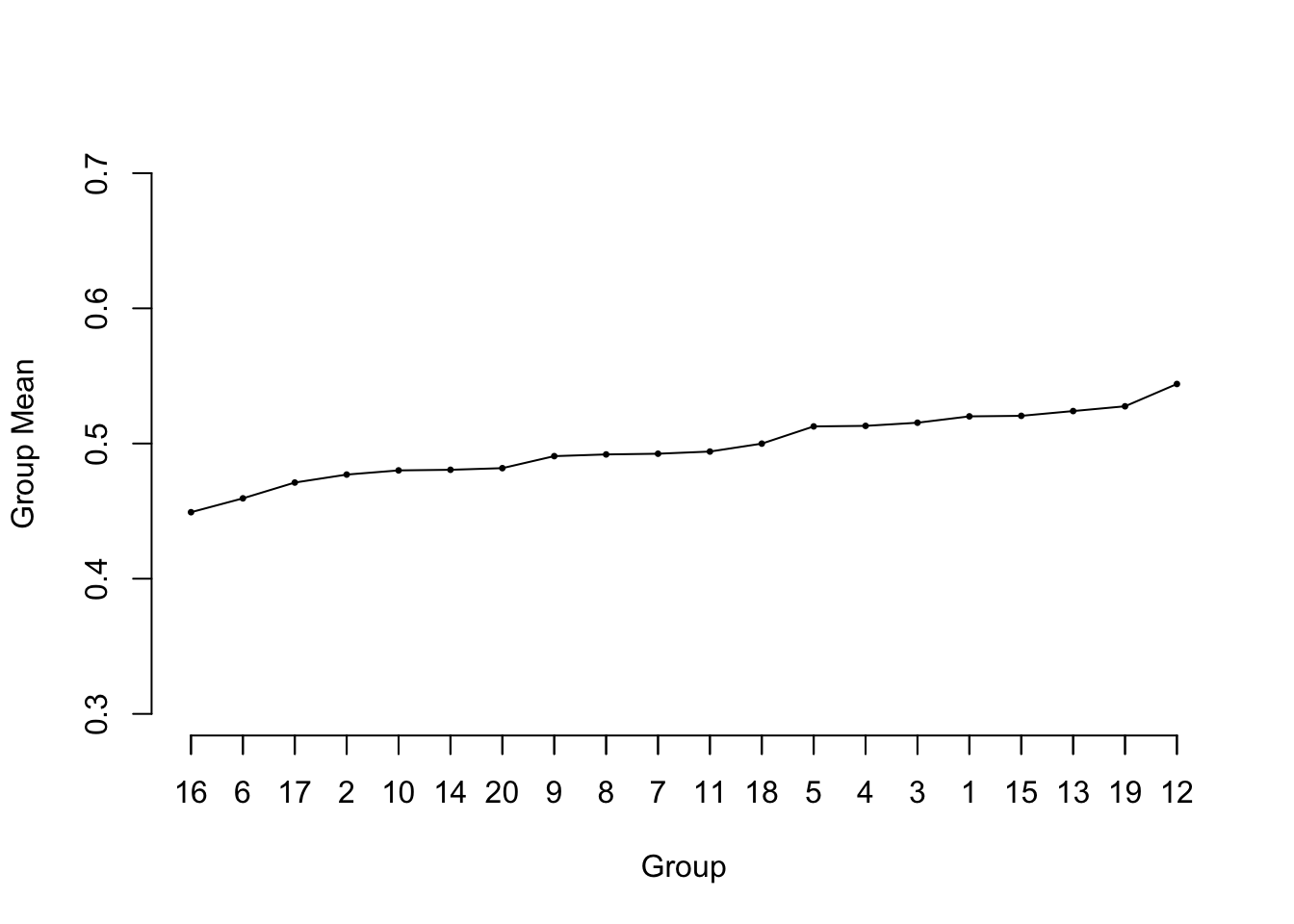
Figure 4.2: Sorted means from 20 samples of size 50 from a uniform \([0,1]\) distribution. The reference line at 0.5 depicts the true population value of all of the means.

• Prevent shrinkage by using pre-shrinkage

• Spiegelhalter (1986): var. selection arbitrary, better prediction usually results from fitting all candidate variables and using shrinkage

• Shrinkage closer to that expected from full model fit than based on number of significant variables (Copas, 1983)

• Ridge regression (le Cessie & van Houwelingen, 1992; van Houwelingen & le Cessie, 1990)

• Penalized MLE (Gray, 1992; Frank E. Harrell et al., 1998; Verweij & van Houwelingen, 1994)

• Heuristic shrinkage parameter of van Houwelingen and le Cessie (van Houwelingen & le Cessie, 1990, Eq. 77) \[\hat{\gamma} = \frac{{\rm model}\ \chi^{2} - p}{{\rm model}\ \chi^{2}}, \tag{4.1}\]

• OLS⁷: \(\hat{\gamma} = \frac{n-p-1}{n-1} R^{2}_{\rm adj} / R^{2}\)
  \(R^{2}_{\rm adj} = 1 - (1 - R^{2})\frac{n-1}{n-p-1}\)

• \(p\) close to no. candidate variables

• Copas (1983) (Eq. 8.5) adds 2 to numerator

VW

⁷ An excellent discussion about such indexes may be found here.

4.6 Collinearity

• When at least 1 predictor can be predicted well from others
• Can be a blessing (data reduction, transformations)
• \(\uparrow\) s.e. of \(\hat{\beta}\), \(\downarrow\) power
• This is appropriate \(\rightarrow\) asking too much of the data (Chatterjee & Hadi, 2012, Chapter 9)
• Variables compete in variable selection, chosen one arbitrary
• Does not affect joint influence of a set of highly correlated variables (use multiple d.f. tests)
• Does not at all affect predictions on model construction sample
• Does not affect predictions on new data (Myers, 1990, pp. 379–381) if
  • Extreme extrapolation not attempted
  • New data have same type of collinearities as original data
• Example: LDL and total cholesterol – problem only if more inconsistent in new data
• Example: age and age\(^{2}\) – no problem
• One way to quantify for each predictor: variance inflation factors (VIF)
• General approach (maximum likelihood) — transform information matrix to correlation form, VIF=diagonal of inverse (Davis et al., 1986; Wax, 1992)
• See David A. Belsley (1991), pp. 28-30 for problems with VIF
• Easy approach: SAS VARCLUS procedure (Sarle, 1990), R varclus function, other clustering techniques: group highly correlated variables
• Can score each group (e.g., first principal component, \(PC_1\) (D’Agostino et al., 1995)); summary scores not collinear

XYZ

4.7 Data Reduction

• Unless \(n>>p\), model unlikely to validate
• Data reduction: \(\downarrow p\)
• Use the literature to eliminate unimportant variables.
• Eliminate variables whose distributions are too narrow.
• Eliminate candidate predictors that are missing in a large number of subjects, especially if those same predictors are likely to be missing for future applications of the model.
• Use a statistical data reduction method such as incomplete principal components regression, nonlinear generalizations of principal components such as principal surfaces, sliced inverse regression, variable clustering, or ordinary cluster analysis on a measure of similarity between variables.
• Data reduction is completely masked to \(Y\), which is precisely why it does not distort estimates, standard errors, \(P\)-values, or confidence limits
• Data reduction = unsupervised learning
• Example: dataset with 40 events and 60 candidate predictors
  • Use variable clustering to group variables by correlation structure
  • Use clinical knowledge to refine the clusters
  • Keep age and severity of disease as separate predictors because of their strength
  • For others create clusters: socioeconomic, risk factors/history, and physiologic function
  • Summarize each cluster with its first principal component \(PC_{1}\), i.e., the linear combination of characteristics that maximizes variance of the score across subjects subject to an overall constraint on the coefficients
  • Fit outcome model with 5 predictors
• See this for useful resources related to principal component analysis of mixed continuous and categorical variables
• See this for an excellent discussion of whether data reduction (unsupervised learning) steps need to be included in resampling for model validation

A

4.7.1 Redundancy Analysis

• Remove variables that have poor distributions
  • E.g., categorical variables with fewer than 2 categories having at least 20 observations
• Use flexible additive parametric additive models to determine how well each variable can be predicted from the remaining variables
• Variables dropped in stepwise fashion, removing the most predictable variable at each step
• Remaining variables used to predict
• Process continues until no variable still in the list of predictors can be predicted with an \(R^2\) or adjusted \(R^2\) greater than a specified threshold or until dropping the variable with the highest \(R^2\) (adjusted or ordinary) would cause a variable that was dropped earlier to no longer be predicted at the threshold from the now smaller list of predictors
• R function redun in Hmisc package
• Related to principal variables (McCabe, 1984) but faster

B

4.7.2 Variable Clustering

• Goal: Separate variables into groups
  • variables within group correlated with each other
  • variables not correlated with non-group members
• Score each dimension, stop trying to separate effects of factors measuring same phenomenon
• Variable clustering (D’Agostino et al., 1995; Sarle, 1990) (oblique-rotation PC analysis) \(\rightarrow\) separate variables so that first PC is representative of group
• Can also do hierarchical cluster analysis on similarity matrix based on squared Spearman or Pearson correlations, or more generally, Hoeffding’s \(D\) (Hoeffding, 1948).
• See Guo et al. (2011) for a method related to variable clustering and sparse principal components.
• Chavent et al. (2012) implement many more variable clustering methods

C

Example: Figure 15.6

4.7.3 Transformation and Scaling Variables Without Using \(Y\)

• Reduce \(p\) by estimating transformations using associations with other predictors

• Purely categorical predictors – correspondence analysis (Ciampi et al., 1986; Crichton & Hinde, 1989; Greenacre, 1988; Leclerc et al., 1988; Michailidis & de Leeuw, 1998)

• Mixture of qualitative and continuous variables: qualitative principal components

• Maximum total variance (MTV) of Young, Takane, de Leeuw (Michailidis & de Leeuw, 1998; Young et al., 1978)

  1. Compute \(PC_1\) of variables using correlation matrix
  2. Use regression (with splines, dummies, etc.) to predict \(PC_1\) from each \(X\) — expand each \(X_j\) and regress it separately on \(PC_1\) to get working transformations
  3. Recompute \(PC_1\) on transformed \(X\)s
  4. Repeat 3-4 times until variation explained by \(PC_1\) plateaus and transformations stabilize

• Maximum generalized variance (MGV) method of Sarle (Kuhfeld, 2009, pp. 1267–1268)

  1. Predict each variable from (current transformations of) all other variables
  2. For each variable, expand it into linear and nonlinear terms or dummies, compute first canonical variate
  3. For example, if there are only two variables \(X_{1}\) and \(X_{2}\) represented as quadratic polynomials, solve for \(a,b,c,d\) such that \(aX_{1}+bX_{1}^{2}\) has maximum correlation with \(cX_{2}+dX_{2}^{2}\).
  4. Goal is to transform each var. so that it is most similar to predictions from other transformed variables
  5. Does not rely on PCs or variable clustering

• MTV (PC-based instead of canonical var.) and MGV implemented in SAS PROC PRINQUAL (Kuhfeld, 2009)

  1. Allows flexible transformations including monotonic splines
  2. Does not allow restricted cubic splines, so may be unstable unless monotonicity assumed
  3. Allows simultaneous imputation but often yields wild estimates

D

4.7.4 Simultaneous Transformation and Imputation

R transcan Function for Data Reduction & Imputation

• Initialize missings to medians (or most frequent category)

• Initialize transformations to original variables

• Take each variable in turn as \(Y\)

• Exclude obs. missing on \(Y\)

• Expand \(Y\) (spline or dummy variables)

• Score (transform \(Y\)) using first canonical variate

• Missing \(Y\) \(\rightarrow\) predict canonical variate from \(X\)s

• The imputed values can optionally be shrunk to avoid overfitting for small \(n\) or large \(p\)

• Constrain imputed values to be in range of non-imputed ones

• Imputations on original scale

  • Continuous \(\rightarrow\) back-solve with linear interpolation
  • Categorical \(\rightarrow\) classification tree (most freq. cat.) or match to category whose canonical score is closest to one predicted

• Multiple imputation — bootstrap or approx. Bayesian bootstrap.

  • Sample residuals multiple times (default \(M=5\))
  • Are on “optimally” transformed scale
  • Back-transform
  • fit.mult.impute works with aregImpute and transcan output to easily get imputation-corrected variances and avg. \(\hat{\beta}\)

• Option to insert constants as imputed values (ignored during transformation estimation); helpful when a lab value may be missing because the patient returned to normal

• Imputations and transformed values may be easily obtained for new data

• An R function Function will create a series of R functions that transform each predictor

• Example: \(n=415\) acutely ill patients

  • Relate heart rate to mean arterial blood pressure
  • Two blood pressures missing
  • Heart rate not monotonically related to blood pressure
  • See Figure 4.3 and Figure 4.4

E

require(Hmisc)
getHdata(support)   # Get data frame from web site
heart.rate     <- support$hrt
blood.pressure <- support$meanbp
blood.pressure[400:401]

Mean Arterial Blood Pressure Day 3 
[1] 151 136

blood.pressure[400:401] <- NA  # Create two missings
d <- data.frame(heart.rate, blood.pressure)
w <- transcan(~ heart.rate + blood.pressure, transformed=TRUE,
              imputed=TRUE, show.na=TRUE, data=d, trantab=TRUE, pl=FALSE)

Convergence criterion:2.901 0.035 0.007 
Convergence in 4 iterations
R-squared achieved in predicting each variable:

    heart.rate blood.pressure 
         0.259          0.259 

Adjusted R-squared:

    heart.rate blood.pressure 
         0.254          0.253 

ggplot(w)
w$imputed$blood.pressure

     400      401 
132.4057 109.7741 

t <- w$transformed
spe <- round(c(spearman(heart.rate, blood.pressure),
               spearman(t[,'heart.rate'],
                        t[,'blood.pressure'])), 2)

Figure 4.3: Transformations fitted using transcan. Tick marks indicate the two imputed values for blood pressure.

spar(mfrow=c(1,2))
plot(heart.rate, blood.pressure)
plot(t[,'heart.rate'], t[,'blood.pressure'],
     xlab='Transformed hr', ylab='Transformed bp')

Figure 4.4: Relationship between heart rate and blood pressure: untransformed data (left) and transformed data (right). Data courtesy of the SUPPORT study (Knaus et al., 1995).

ACE (Alternating Conditional Expectation) of L. Breiman & Friedman (1985)

1. Uses nonparametric “super smoother” (Friedman, 1984)
2. Allows monotonicity constraints, categorical vars.
3. Does not handle missing data

F

• These methods find marginal transformations

• Check adequacy of transformations using \(Y\)

  • Graphical
  • Nonparametric smoothers (\(X\) vs. \(Y\))
  • Expand original variable using spline, test additional predictive information over original transformation

G

4.7.5 Simple Scoring of Variable Clusters

• Try to score groups of transformed variables with \(PC_1\)
• Reduces d.f. by pre-transforming var. and by combining multiple var.
• Later may want to break group apart, but delete all variables in groups whose summary scores do not add significant information
• Sometimes simplify cluster score by finding a subset of its constituent variables which predict it with high \(R^2\).

H

Series of dichotomous variables:

• Construct \(X_1\) = 0-1 according to whether any variables positive
• Construct \(X_2\) = number of positives
• Test whether original variables add to \(X_1\) or \(X_2\)

I

4.7.6 Simplifying Cluster Scores

4.7.7 How Much Data Reduction Is Necessary?

Using Expected Shrinkage to Guide Data Reduction

• Fit full model with all candidates, \(p\) d.f., LR likelihood ratio \(\chi^2\)
• Compute \(\hat{\gamma}\)
• If \(<0.9\), consider shrunken estimator from whole model, or data reduction (again not using \(Y\))
• \(q\) regression d.f. for reduced model
• Assume best case: discarded dimensions had no association with \(Y\)
• Expected loss in LR is \(p-q\)
• New shrinkage \([{\rm LR} - (p-q) - q]/[{\rm LR} - (p-q)]\)
• Solve for \(q\) \(\rightarrow\) \(q \leq ({\rm LR}-p)/9\)
• Under these assumptions, no hope unless original LR \(> p+9\)
• No \(\chi^2\) lost by dimension reduction \(\rightarrow\) \(q \leq {\rm LR}/10\)

J

Example:

• Binary logistic model, 45 events on 150 subjects
• 10:1 rule \(\rightarrow\) analyze 4.5 d.f. total
• Analyst wishes to include age, sex, 10 others
• Not known if age linear or if age and sex additive
• 4 knots \(\rightarrow\) \(3+1+1\) d.f. for age and sex if restrict interaction to be linear
• Full model with 15 d.f. has LR=50
• Expected shrinkage factor \((50-15)/50 = 0.7\)
• LR\(>15+9=24\) \(\rightarrow\) reduction may help
• Reduction to \(q = (50-15)/9 \approx 4\) d.f. necessary
• Have to assume age linear, reduce other 10 to 1 d.f.
• Separate hypothesis tests intended \(\rightarrow\) use full model, adjust for multiple comparisons

K

Summary of Some Data Reduction Methods

Goals	Reasons	Methods
Group predictors so that each group represents a single dimension that can be summarized with a single score	• \(\downarrow\) d.f. arising from multiple predictors • Make \(PC_1\) more reasonable summary	Variable clustering • Subject matter knowledge • Group predictors to maximize proportion of variance explained by \(PC_1\) of each group • Hierarchical clustering using a matrix of similarity measures between predictors
Transform predictors	• \(\downarrow\) d.f. due to nonlinear and dummy variable components • Allows predictors to be optimally combined • Make \(PC_1\) more reasonable summary • Use in customized model for imputing missing values on each predictor	• Maximum total variance on a group of related predictors • Canonical variates on the total set of predictors

4.8 Other Approaches to Predictive Modeling

4.9 Overly Influential Observations

• Every observation should influence fit
• Major results should not rest on 1 or 2 obs.
• Overly infl. obs. \(\rightarrow\) \(\uparrow\) variance of predictions
• Also affects variable selection

L

Reasons for influence:

• Too few observations for complexity of model (see Section 4.7, Section 4.3)
• Data transcription or entry errors
• Extreme values of a predictor

M

1. Sometimes subject so atypical should remove from dataset
2. Sometimes truncate measurements where data density ends
3. Example: \(n=4000\), 2000 deaths, white blood count range 500-100,000, .05,.95 quantiles=2755, 26700
4. Linear spline function fit
5. Sensitive to WBC\(>60000\ (n=16)\)
6. Predictions stable if truncate WBC to 40000 (\(n=46\) above 40000)

• Disagreements between predictors and response. Ignore unless extreme values or another explanation
• Example: \(n=8000\), one extreme predictor value not on straight line relationship with other \((X,Y)\) \(\rightarrow\) \(\chi^{2}=36\) for \(H_{0}:\) linearity

Statistical Measures:

• Leverage: capacity to be influential (not necessarily infl.)
  Diagonals of “hat matrix” \(H = X(X'X)^{-1}X'\) — measures how an obs. predicts its own response (D. A. Belsley et al., 1980)
• \(h_{ii}>2(p+1)/n\) may signal a high leverage point (D. A. Belsley et al., 1980)
• DFBETAS: change in \(\hat{\beta}\) upon deletion of each obs, scaled by s.e.
• DFFIT: change in \(X\hat{\beta}\) upon deletion of each obs
• DFFITS: DFFIT standardized by s.e. of \(\hat{\beta}\)
• Some classify obs as overly influential when \(|{\rm DFFITS}|>2\sqrt{(p+1)/(n-p-1)}\) (D. A. Belsley et al., 1980)
• Others examine entire distribution for “outliers”
• No substitute for careful examination of data (Chatfield, 1991; Spence & Garrison, 1993)
• Maximum likelihood estimation requires 1-step approximations

N

4.10 Comparing Two Models

• Level playing field (independent datasets, same no. candidate d.f., careful bootstrapping)
• Criteria:
  1. calibration
  2. discrimination
  3. face validity
  4. measurement errors in required predictors
  5. use of continuous predictors (which are usually better defined than categorical ones)
  6. omission of “insignificant” variables that nonetheless make sense as risk factors
  7. simplicity (though this is less important with the availability of computers)
  8. lack of fit for specific types of subjects
• Goal is to rank-order: ignore calibration
• Otherwise, dismiss a model having poor calibration
• Good calibration \(\rightarrow\) compare discrimination (e.g., \(R^{2}\) (Nagelkerke, 1991), model \(\chi^2\), Somers’ \(D_{xy}\), Spearman’s \(\rho\), area under ROC curve)
• Worthwhile to compare models on a measure not used to optimize either model, e.g., mean absolute error, median absolute error if using OLS
• Rank measures may not give enough credit to extreme predictions \(\rightarrow\) model \(\chi^{2}, R^{2}\), examine extremes of distribution of \(\hat{Y}\)
• Examine differences in predicted values from the two models
• See (Peek et al., 2007; Pencina et al., 2008, 2011, 2012) for discussions and examples of low power for testing differences in ROC areas, and for other approaches.

OPQ

4.11 Improving the Practice of Multivariable Prediction

See also Section 5.6

Greenland (2000) discusses many important points:

• Stepwise variable selection on confounders leaves important confounders uncontrolled
• Shrinkage is far superior to variable selection
• Variable selection does more damage to confidence interval widths than to point estimates
• Claims about unbiasedness of ordinary MLEs are misleading because they assume the model is correct and is the only model entertained
• “models need to be complex to capture uncertainty about the relations … an honest uncertainty assessment requires parameters for all effects that we know may be present. This advice is implicit in an anti-parsimony principle often attributed to L. J. Savage ‘All models should be as big as an elephant’ (see Draper, 1995)”

R

Greenland’s example of inadequate adjustment for confounders as a result of using a bad modeling strategy:

• Case-control study of diet, food constituents, breast cancer
• 140 cases, 222 controls
• 35 food constituent intakes and 5 confounders
• Food intakes are correlated
• Traditional stepwise analysis not adjusting simultaneously for all foods consumed \(\rightarrow\) 11 foods had \(P < 0.05\)
• Full model with all 35 foods competing \(\rightarrow\) 2 had \(P < 0.05\)
• Rigorous simultaneous analysis (hierarchical random slopes model) penalizing estimates for the number of associations examined \(\rightarrow\) no foods associated with breast cancer

S

Global Strategies

• Use a method known not to work well (e.g., stepwise variable selection without penalization; recursive partitioning), document how poorly the model performs (e.g. using the bootstrap), and use the model anyway
• Develop a black box model that performs poorly and is difficult to interpret (e.g., does not incorporate penalization)
• Develop a black box model that performs well and is difficult to interpret
• Develop interpretable approximations to the black box
• Develop an interpretable model (e.g. give priority to additive effects) that performs well and is likely to perform equally well on future data from the same stream

T

Preferred Strategy in a Nutshell

• Decide how many d.f. can be spent
• Decide where to spend them
• Spend them
• Don’t reconsider, especially if inference needed

U

4.12 Summary: Possible Modeling Strategies

4.12.1 Developing Predictive Models

1. Assemble accurate, pertinent data and lots of it, with wide distributions for \(X\).
2. Formulate good hypotheses — specify relevant candidate predictors and possible interactions. Don’t use \(Y\) to decide which \(X\)’s to include.
3. Characterize subjects with missing \(Y\). Delete such subjects in rare circumstances (Crawford et al., 1995). For certain models it is effective to multiply impute \(Y\).
4. Characterize and impute missing \(X\). In most cases use multiple imputation based on \(X\) and \(Y\)
5. For each predictor specify complexity or degree of nonlinearity that should be allowed (more for important predictors or for large \(n\)) (Section 4.1)
6. Do data reduction if needed (pre-transformations, combinations), or use penalized estimation (Frank E. Harrell et al., 1998)
7. Use the entire sample in model development
8. Can do highly structured testing to simplify “initial” model
   • Test entire group of predictors with a single \(P\)-value
   • Make each continuous predictor have same number of knots, and select the number that optimizes AIC
   • Test the combined effects of all nonlinear terms with a single \(P\)-value
9. Make tests of linearity of effects in the model only to demonstrate to others that such effects are often statistically significant. Don’t remove individual insignificant effects from the model.
10. Check additivity assumptions by testing pre-specified interaction terms. Use a global test and either keep all or delete all interactions.
11. Check to see if there are overly-influential observations.
12. Check distributional assumptions and choose a different model if needed.
13. Do limited backwards step-down variable selection if parsimony is more important that accuracy (Spiegelhalter, 1986). But confidence limits, etc., must account for variable selection (e.g., bootstrap).
14. This is the “final” model.
15. Interpret the model graphically and by computing predicted values and appropriate test statistics. Compute pooled tests of association for collinear predictors.
16. Validate this model for calibration and discrimination ability, preferably using bootstrapping.
17. Shrink parameter estimates if there is overfitting but no further data reduction is desired (unless shrinkage built-in to estimation)
18. When missing values were imputed, adjust final variance-covariance matrix for imputation. Do this as early as possible because it will affect other findings.
19. When all steps of the modeling strategy can be automated, consider using Faraway (1992) to penalize for the randomness inherent in the multiple steps.
20. Develop simplifications to the final model as needed.

V

4.12.2 Developing Models for Effect Estimation

1. Less need for parsimony; even less need to remove insignificant variables from model (otherwise CLs too narrow)
2. Careful consideration of interactions; inclusion forces estimates to be conditional and raises variances
3. If variable of interest is mostly the one that is missing, multiple imputation less valuable
4. Complexity of main variable specified by prior beliefs, compromise between variance and bias
5. Don’t penalize terms for variable of interest
6. Model validation less necessary
7. Like the hypothesis testing scenario covered next, when one is attempting to apply a causal interpretation to the effect being estimated, consideration of pathways and confounding are all-important. Collider bias and backdoor pathways can ruin interpretation, and so can the omission of confounder variables that would have provided alternate explanations for observed effects of interest. In pure prediction mode we don’t care very much how we got here, but in isolating the effect of a specific variable in the model, e.g., in estimating the effect of treatment in an observational treatment comparison study, measuring and adjusting for nearly all confounding in play are very important. Sometimes adjusting for confounding requires overfitting the model from a prediction standpoint, but that is OK. Overfitting can result in widering confidence intervals for the effect of interest, and that is a proper price to pay.

W

4.12.3 Developing Models for Hypothesis Testing

1. Virtually same as previous strategy
2. Interactions require tests of effect by varying values of another variable, or “main effect + interaction” joint tests (e.g., is treatment effective for either sex, allowing effects to be different)
3. Validation may help quantify over-adjustment

X

4.13 Study Questions

Section 4.1

1. An investigator is interested in finding risk factors for stroke. She has collected data on 3000 subjects of whom 70 were known to suffer a stroke within 5 years from study entry. She has decided that race (5 possible levels), age, height, and mean arterial blood pressure should definitely be in the model. She does not try to find previous studies that show how these potential risk factors relate to the risk of stroke. What is one way to decide how many degrees of freedom to spend on each predictor? How can one achieve these d.f. (whatever they are) for race and for a continuous variable?
2. What is the driving force behind the approach used here to prespecify the complexity with which each predictor is specified in the regression model?
3. Why is the process fair?
4. When feasible to do, why is learning from a saturated model preferred?

Section 4.3

1. What did we already study that variable selection is an extension of?
2. What does variable selection ruin more than it ruins regression coefficient estimates?
3. Besides those problems what’s the worst thing you can say about statistical test-based variable selection?
4. In which situation would variable selection have a chance to be helpful?
5. What is the statistical point that the Maxwell demon analogy is trying to bring out?
6. What is the single root cause of problems that is in common to each of the following strategies?
   • The investigator retains race as 5 categories and fits it with 4 dummy variables. She examines coefficients from these dummy variables to decide which races have similar coefficients and should be pooled.
   • All continuous variables are allowed to be nonlinear using splines, and variables having insignificant nonlinear terms are re-fitted as linear.
   • All potential risk factors are used as candidate predictor variables with forward stepwise variable selection with a significance level for entering the model of \(\alpha=0.1\).
   • A clinical trial of 5 treatments find that 3 of the treatments result in nearly the same blood pressure reduction. These 3 treatments are pooled and their overall mean is compared with each of the remaining 2 treatments.
7. Name at least one specific harm done by the strategies outlined in the last question, in general terms (not specific to each strategy).

Section 4.4

1. Describe a major way that “breaking ties” in Y, i.e., having it more continuous, results in more power and precision in modeling.
2. What is the effective sample size in a study with 10 cancer outcomes and 100,000 normal outcomes?

Section 4.5

1. What are main causes of passive shrinkage/regression to the mean?
2. Why does the heuristic shrinkage estimate work?
3. What causes the graph of \(\hat{Y}\) (on \(x\)-axis) vs. \(Y\) (on \(y\)-axis; you could call this \(Y_{new}\)) to be flatter than a \(45^\circ\) line when the graph is made for new data not used to fit the model?

Section 4.6

1. What causes the standard error of a regression coefficient to get large when adjusting for a competing predictor?
2. When just wanting to measure strength of association or test a group of predictors, what is a simple fix for co-linearity?

Section 4.7

1. What is the purpose of data reduction, and why does it not create phantom degrees of freedom that need to be accounted for later in the modeling process?
2. Name several data reduction methods for reducing the number of regression coefficients to estimate.
3. Principal components can have unstable loadings (e.g., if you bootstrap). Why are they still a valuable component in a data reduction strategy?
4. What is the overall guidance for knowing how much unsupervised learning (data reduction) to do?

Section 4.9

1. Why are high leverage (far out) observations influential on regression coefficients even when Y is binary?

Section 4.10

1. What would make one model having much better predictive discrimination than another irrelevant?

Section 4.12

1. Are the steps to the default strategy complete and is the sequencing “correct”?

Altman, D. G., & Andersen, P. K. (1989). Bootstrap investigation of the stability of a Cox regression model. Stat Med, 8, 771–783.

Atkinson, A. C. (1980). A note on the generalized information criterion for choice of a model. Biometrika, 67, 413–418.

Austin, P. C. (2008). Bootstrap model selection had similar performance for selecting authentic and noise variables compared to backward variable elimination: A simulation study. J Clin Epi, 61, 1009–1017.

"in general, a bootstrap model selection method had comparable performance to conventional backward variable elimination for identifying the true regression model. In most settings, both methods performed poorly at correctly identifying the correct regression model."

Belsley, David A. (1991). Conditioning Diagnostics: Collinearity and Weak Data in Regression. Wiley.

Belsley, D. A., Kuh, E., & Welsch, R. E. (1980). Regression Diagnostics: Identifying Influential Data and Sources of Collinearity. Wiley.

Benedetti, J. K., Liu, P.-Y., Sather, H. N., Seinfeld, J., & Epton, M. A. (1982). Effective sample size for tests of censored survival data. Biometrika, 69, 343–349.

Breiman, Leo. (1992). The little bootstrap and other methods for dimensionality selection in regression: X-fixed prediction error. J Am Stat Assoc, 87, 738–754.

Breiman, L., & Friedman, J. H. (1985). Estimating optimal transformations for multiple regression and correlation (with discussion). J Am Stat Assoc, 80, 580–619.

Chatfield, C. (1991). Avoiding statistical pitfalls (with discussion). Stat Sci, 6, 240–268.

Chatfield, C. (1995). Model uncertainty, data mining and statistical inference (with discussion). J Roy Stat Soc A, 158, 419–466.

bias by selecting model because it fits the data well; bias in standard errors;P. 420: ... need for a better balance in the literature and in statistical teaching between  techniques and problem solving  strategies. P. 421: It is “well known” to be “logically unsound and practically misleading” (Zhang, 1992) to make inferences as if a model is known to be true when it has, in fact, been selected from the  same data to be used for estimation purposes. However, although statisticians may admit this privately (Breiman (1992) calls it a “quiet scandal”), they (we) continue to ignore the difficulties because it is not clear what else could or should be done. P. 421: Estimation errors for regression coefficients are usually smaller than errors from failing to take into account model specification. P. 422: Statisticians must stop pretending that model uncertainty does not exist and begin to find ways of coping with it. P. 426: It is indeed strange that we often admit model uncertainty by searching for a best model but then ignore this uncertainty by making inferences and predictions as if certain that the best fitting model is actually true. P. 427: The analyst needs to assess the model selection  process and not just the best fitting model. P. 432: The use of subset selection methods is well known to introduce alarming biases. P. 433: ... the AIC can be highly biased in data-driven model selection situations. P. 434: Prediction intervals will generally be too narrow. In the discussion, Jamal R. M. Ameen states that a model should be (a) satisfactory in performance relative to the stated objective, (b) logically sound, (c) representative, (d) questionable and subject to on-line interrogation, (e) able to accommodate external or expert information and (f) able to convey information.

Chatterjee, S., & Hadi, A. S. (2012). Regression Analysis by Example (Fifth). Wiley.

Chavent, M., Kuentz-Simonet, V., Liquet, B., & Saracco, J. (2012). ClustOfVar: An R package for the clustering of variables. J Stat Software, 50(13), 1–16.

Ciampi, A., Thiffault, J., Nakache, J. P., & Asselain, B. (1986). Stratification by stepwise regression, correspondence analysis and recursive partition. Comp Stat Data Analysis, 1986, 185–204.

Copas, J. B. (1983). Regression, prediction and shrinkage (with discussion). J Roy Stat Soc B, 45, 311–354.

Crawford, S. L., Tennstedt, S. L., & McKinlay, J. B. (1995). A comparison of analytic methods for non-random missingness of outcome data. J Clin Epi, 48, 209–219.

Crichton, N. J., & Hinde, J. P. (1989). Correspondence analysis as a screening method for indicants for clinical diagnosis. Stat Med, 8, 1351–1362.

D’Agostino, R. B., Belanger, A. J., Markson, E. W., Kelly-Hayes, M., & Wolf, P. A. (1995). Development of health risk appraisal functions in the presence of multiple indicators: The Framingham Study nursing home institutionalization model. Stat Med, 14, 1757–1770.

Davis, C. E., Hyde, J. E., Bangdiwala, S. I., & Nelson, J. J. (1986). An example of dependencies among variables in a conditional logistic regression. In S. H. Moolgavkar & R. L. Prentice (Eds.), Modern Statistical Methods in Chronic Disease Epidemiology (pp. 140–147). Wiley.

Derksen, S., & Keselman, H. J. (1992). Backward, forward and stepwise automated subset selection algorithms: Frequency of obtaining authentic and noise variables. British J Math Stat Psych, 45, 265–282.

Faraway, J. J. (1992). The cost of data analysis. J Comp Graph Stat, 1, 213–229.

Friedman, J. H. (1984). A variable span smoother (Technical Report No. 5). Laboratory for Computational Statistics, Department of Statistics, Stanford University.

Giudice, J. H., Fieberg, J. R., & Lenarz, M. S. (2011). Spending degrees of freedom in a poor economy: A case study of building a sightability model for moose in northeastern minnesota. J Wildlife Manage. https://doi.org/10.1002/jwmg.213

Grambsch, P. M., & O’Brien, P. C. (1991). The effects of transformations and preliminary tests for non-linearity in regression. Stat Med, 10, 697–709.

Gray, R. J. (1992). Flexible methods for analyzing survival data using splines, with applications to breast cancer prognosis. J Am Stat Assoc, 87, 942–951.

Greenacre, M. J. (1988). Correspondence analysis of multivariate categorical data by weighted least-squares. Biometrika, 75, 457–467.

Greenland, S. (2000). When should epidemiologic regressions use random coefficients? Biometrics, 56, 915–921. https://doi.org/10.1111/j.0006-341X.2000.00915.x

use of statistics in epidemiology is largely primitive;stepwise variable selection on confounders leaves important confounders uncontrolled;composition matrix;example with far too many significant predictors with many regression coefficients absurdly inflated when overfit;lack of evidence for dietary effects mediated through constituents;shrinkage instead of variable selection;larger effect on confidence interval width than on point estimates with variable selection;uncertainty about variance of random effects is just uncertainty about prior opinion;estimation of variance is pointless;instead the analysis should be repeated using different values;"if one feels compelled to estimate $\tau{̂2}$, I would recommend giving it a proper prior concentrated amount contextually reasonable values";claim about ordinary MLE being unbiased is misleading because it assumes the model is correct and is the only model entertained;shrinkage towards compositional model;"models need to be complex to capture uncertainty about the relations...an honest uncertainty assessment requires parameters for all effects that we know may be present. This advice is implicit in an antiparsimony principle often attributed to L. J. Savage ’All models should be as big as an elephant (see Draper, 1995)’". See also gus06per.

Guo, J., James, G., Levina, E., Michailidis, G., & Zhu, J. (2011). Principal component analysis with sparse fused loadings. J Comp Graph Stat, 19(4), 930–946.

incorporates blocking structure in the variables;selects different variables for different components;encourages loadings of highly correlated variables to have same magnitude, which aids in interpretation

Harrell, F. E. (1986). The LOGIST Procedure. In SUGI Supplemental Library Users Guide (Version 5, pp. 269–293). SAS Institute, Inc.

Harrell, F. E., Lee, K. L., Califf, R. M., Pryor, D. B., & Rosati, R. A. (1984). Regression modeling strategies for improved prognostic prediction. Stat Med, 3, 143–152.

Harrell, Frank E., Lee, K. L., & Mark, D. B. (1996). Multivariable prognostic models: Issues in developing models, evaluating assumptions and adequacy, and measuring and reducing errors. Stat Med, 15, 361–387.

Harrell, F. E., Lee, K. L., Matchar, D. B., & Reichert, T. A. (1985). Regression models for prognostic prediction: Advantages, problems, and suggested solutions. Ca Trt Rep, 69, 1071–1077.

Harrell, Frank E., Margolis, P. A., Gove, S., Mason, K. E., Mulholland, E. K., Lehmann, D., Muhe, L., Gatchalian, S., & Eichenwald, H. F. (1998). Development of a clinical prediction model for an ordinal outcome: The World Health Organization ARI Multicentre Study of clinical signs and etiologic agents of pneumonia, sepsis, and meningitis in young infants. Stat Med, 17, 909–944. http://onlinelibrary.wiley.com/doi/10.1002/(SICI)1097-0258(19980430)17:8%3C909::AID-SIM753%3E3.0.CO;2-O/abstract

Hoeffding, W. (1948). A non-parametric test of independence. Ann Math Stat, 19, 546–557.

Hurvich, C. M., & Tsai, C. L. (1990). The impact of model selection on inference in linear regression. Am Statistician, 44, 214–217.

Knaus, W. A., Harrell, F. E., Lynn, J., Goldman, L., Phillips, R. S., Connors, A. F., Dawson, N. V., Fulkerson, W. J., Califf, R. M., Desbiens, N., Layde, P., Oye, R. K., Bellamy, P. E., Hakim, R. B., & Wagner, D. P. (1995). The SUPPORT prognostic model: Objective estimates of survival for seriously ill hospitalized adults. Ann Int Med, 122, 191–203. https://doi.org/10.7326/0003-4819-122-3-199502010-00007

Kuhfeld, W. F. (2009). The PRINQUAL Procedure. In SAS/STAT 9.2 User’s Guide (Second). SAS Publishing. http://support.sas.com/documentation/onlinedoc/stat

Lawless, J. F., & Singhal, K. (1978). Efficient screening of nonnormal regression models. Biometrics, 34, 318–327.

le Cessie, S., & van Houwelingen, J. C. (1992). Ridge estimators in logistic regression. Appl Stat, 41, 191–201.

Leclerc, A., Luce, D., Lert, F., Chastang, J. F., & Logeay, P. (1988). Correspondence analysis and logistic modelling: Complementary use in the analysis of a health survey among nurses. Stat Med, 7, 983–995.

Lockhart, R., Taylor, J., Tibshirani, R. J., & Tibshirani, R. (2013). A significance test for the lasso. arXiv. http://arxiv.org/abs/1301.7161

Mantel, N. (1970). Why stepdown procedures in variable selection. Technometrics, 12, 621–625.

McCabe, G. P. (1984). Principal variables. Technometrics, 26, 137–144.

Michailidis, G., & de Leeuw, J. (1998). The Gifi system of descriptive multivariate analysis. Stat Sci, 13, 307–336.

Myers, R. H. (1990). Classical and Modern Regression with Applications. PWS-Kent.

Nagelkerke, N. J. D. (1991). A note on a general definition of the coefficient of determination. Biometrika, 78, 691–692.

Nick, T. G., & Hardin, J. M. (1999). Regression modeling strategies: An illustrative case study from medical rehabilitation outcomes research. Am J Occ Ther, 53, 459–470.

Peduzzi, P., Concato, J., Feinstein, A. R., & Holford, T. R. (1995). Importance of events per independent variable in proportional hazards regression analysis. II. Accuracy and precision of regression estimates. J Clin Epi, 48, 1503–1510.

Peduzzi, P., Concato, J., Kemper, E., Holford, T. R., & Feinstein, A. R. (1996). A simulation study of the number of events per variable in logistic regression analysis. J Clin Epi, 49, 1373–1379.

Peek, N., Arts, D. G. T., Bosman, R. J., van der Voort, P. H. J., & de Keizer, N. F. (2007). External validation of prognostic models for critically ill patients required substantial sample sizes. J Clin Epi, 60, 491–501.

large sample sizes need to obtain reliable external validations;inadequate power of DeLong, DeLong, and Clarke-Pearson test for differences in correlated ROC areas (p. 498);problem with tests of calibration accuracy having too much power for large sample sizes

Pencina, M. J., D’Agostino, R. B., & Demler, O. V. (2012). Novel metrics for evaluating improvement in discrimination: Net reclassification and integrated discrimination improvement for normal variables and nested models. Stat Med, 31(2), 101–113. https://doi.org/10.1002/sim.4348

Pencina, M. J., D’Agostino, R. B., & Steyerberg, E. W. (2011). Extensions of net reclassification improvement calculations to measure usefulness of new biomarkers. Stat Med, 30, 11–21. https://doi.org/10.1002/sim.4085

lack of need for NRI to be category-based;arbitrariness of categories;"category-less or continuous NRI is the most objective and versatile measure of improvement in risk prediction;authors misunderstood the inadequacy of three categories if categories are used;comparison of NRI to change in C index;example of continuous plot of risk for old model vs. risk for new model

Pencina, M. J., D’Agostino Sr, R. B., D’Agostino Jr, R. B., & Vasan, R. S. (2008). Evaluating the added predictive ability of a new marker: From area under the ROC curve to reclassification and beyond. Stat Med, 27, 157–172.

small differences in ROC area can still be very meaningful;example of insignificant test for difference in ROC areas with very significant results from new method;Yates’ discrimination slope;reclassification table;limiting version of this based on whether and amount by which probabilities rise for events and lower for non-events when compare new model to old;comparing two models;see letter to the editor by Van Calster and Van Huffel, Stat in Med 29:318-319, 2010 and by Cook and Paynter, Stat in Med 31:93-97, 2012

Riley, R. D., Snell, K. I., Ensor, J., Burke, D. L., Harrell, F. E., Moons, K. G., & Collins, G. S. (2019). Minimum sample size for developing a multivariable prediction model: PART II - binary and time-to-event outcomes. Stat Med, 38(7), 1276–1296. https://doi.org/10.1002/sim.7992

Riley, R. D., Snell, K. I., Ensor, J., Burke, D. L., Jr, F. E. H., Moons, K. G., & Collins, G. S. (2019). Minimum sample size for developing a multivariable prediction model: PART II - binary and time-to-event outcomes. Statistics in Medicine, 38(7), 1276–1296. https://doi.org/10.1002/sim.7992

Roecker, E. B. (1991). Prediction error and its estimation for subset-selected models. Technometrics, 33, 459–468.

Sarle, W. (1990). The VARCLUS Procedure. In SAS/STAT User’s Guide (fourth, Vol. 2, pp. 1641–1659). SAS Institute, Inc. http://support.sas.com/documentation/onlinedoc/stat

Sauerbrei, W., & Schumacher, M. (1992). A bootstrap resampling procedure for model building: Application to the Cox regression model. Stat Med, 11, 2093–2109.

Smith, L. R., Harrell, F. E., & Muhlbaier, L. H. (1992). Problems and potentials in modeling survival. In M. L. Grady & H. A. Schwartz (Eds.), Medical Effectiveness Research Data Methods (Summary Report), AHCPR Pub. No. 92-0056 (pp. 151–159). US Dept. of Health and Human Services, Agency for Health Care Policy and Research. https://hbiostat.org/bib/papers/smi92pro.pdf

Spence, I., & Garrison, R. F. (1993). A remarkable scatterplot. Am Statistician, 47, 12–19.

Spiegelhalter, D. J. (1986). Probabilistic prediction in patient management and clinical trials. Stat Med, 5, 421–433. https://doi.org/10.1002/sim.4780050506

z-test for calibration inaccuracy (implemented in Stata, and R Hmisc package’s val.prob function)

Steyerberg, E. W., Eijkemans, M. J. C., Harrell, F. E., & Habbema, J. D. F. (2001). Prognostic modeling with logistic regression analysis: In search of a sensible strategy in small data sets. Med Decis Mak, 21, 45–56.

Sun, G.-W., Shook, T. L., & Kay, G. L. (1996). Inappropriate use of bivariable analysis to screen risk factors for use in multivariable analysis. J Clin Epi, 49, 907–916.

van der Ploeg, T., Austin, P. C., & Steyerberg, E. W. (2014). Modern modelling techniques are data hungry: A simulation study for predicting dichotomous endpoints. BMC Medical Research Methodology, 14(1), 137+. https://doi.org/10.1186/1471-2288-14-137

Would be better to use proper accuracy scores in the assessment. Too much emphasis on optimism as opposed to final discrimination measure. But much good practical information. Recursive partitioning fared poorly.

van Houwelingen, J. C., & le Cessie, S. (1990). Predictive value of statistical models. Stat Med, 9, 1303–1325.

Verweij, P. J., & van Houwelingen, H. C. (1994). Penalized likelihood in Cox regression. Stat Med, 13, 2427–2436.

Vittinghoff, E., & McCulloch, C. E. (2006). Relaxing the rule of ten events per variable in logistic and Cox regression. Am J Epi, 165, 710–718.

the authors may have not been quite stringent enough in their assessment of adequacy of predictions;letter to the editor submitted

Wax, Y. (1992). Collinearity diagnosis for a relative risk regression analysis: An application to assessment of diet-cancer relationship in epidemiological studies. Stat Med, 11, 1273–1287.

Whitehead, J. (1993). Sample size calculations for ordered categorical data. Stat Med, 12, 2257–2271.

Wiegand, R. E. (2010). Performance of using multiple stepwise algorithms for variable selection. Stat Med, 29, 1647–1659.

fruitless to try different stepwise methods and look for agreement;the methods will agree on the wrong model

Young, F. W., Takane, Y., & de Leeuw, J. (1978). The principal components of mixed measurement level multivariate data: An alternating least squares method with optimal scaling features. Psychometrika, 43, 279–281.