Code
require(rms)
S <- Surv(c(1, 3, 3, 6, 8, 9, 10), c(1,1,1,0,0,1,0))
fe <- psm(S ~ 1, dist='exponential')
f2 <- psm(S ~ 1, dist='weibull')Why use a parametric model?
Note: Fitting more than two smooth survival curves and choosing the one that best reproduces the KM estimator will result in a true precision no better than KM due to model uncertainty.
\[ \log L = \sum_{i:Y_{i} {\rm\ uncensored}}^{n} \log \lambda - \sum_{i=1}^{n} \lambda Y_{i} \]
\[\begin{array}{ccc} \hat{\lambda} &=& n_{u}/w \\ {\rm var}(\hat{\lambda}) &=& n_{u}/w^{2} \\ {\rm var}(\log \hat{\lambda}) &=& 1/n_{u} \\ \hat{\mu} &=& w/n_{u} \\ \hat{S}(t) &=& \exp(-\hat{\lambda}t) \end{array}\]Consider these failure time data:
\[\begin{array}{c} 1 \ \ 3\ \ 3\ \ 6^{+}\ \ 8^{+}\ \ 9\ \ 10^{+} . \nonumber \end{array}\]require(rms)
S <- Surv(c(1, 3, 3, 6, 8, 9, 10), c(1,1,1,0,0,1,0))
fe <- psm(S ~ 1, dist='exponential')
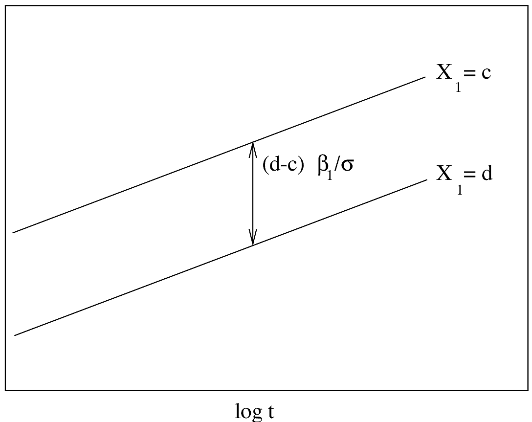
f2 <- psm(S ~ 1, dist='weibull')\[ \log[-\log S(t)] = \log \Lambda(t) = \log \alpha +\gamma (\log t) \]
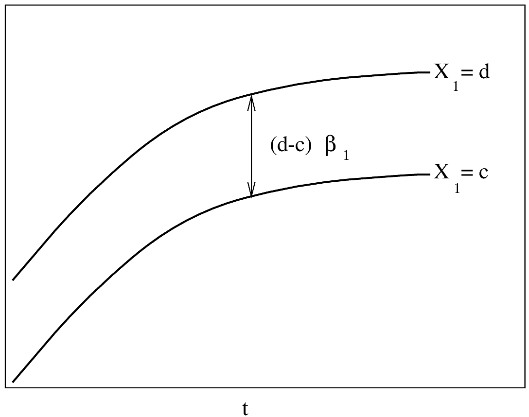
\[ \lambda(t|X) = \lambda(t) \exp(X\beta) \]
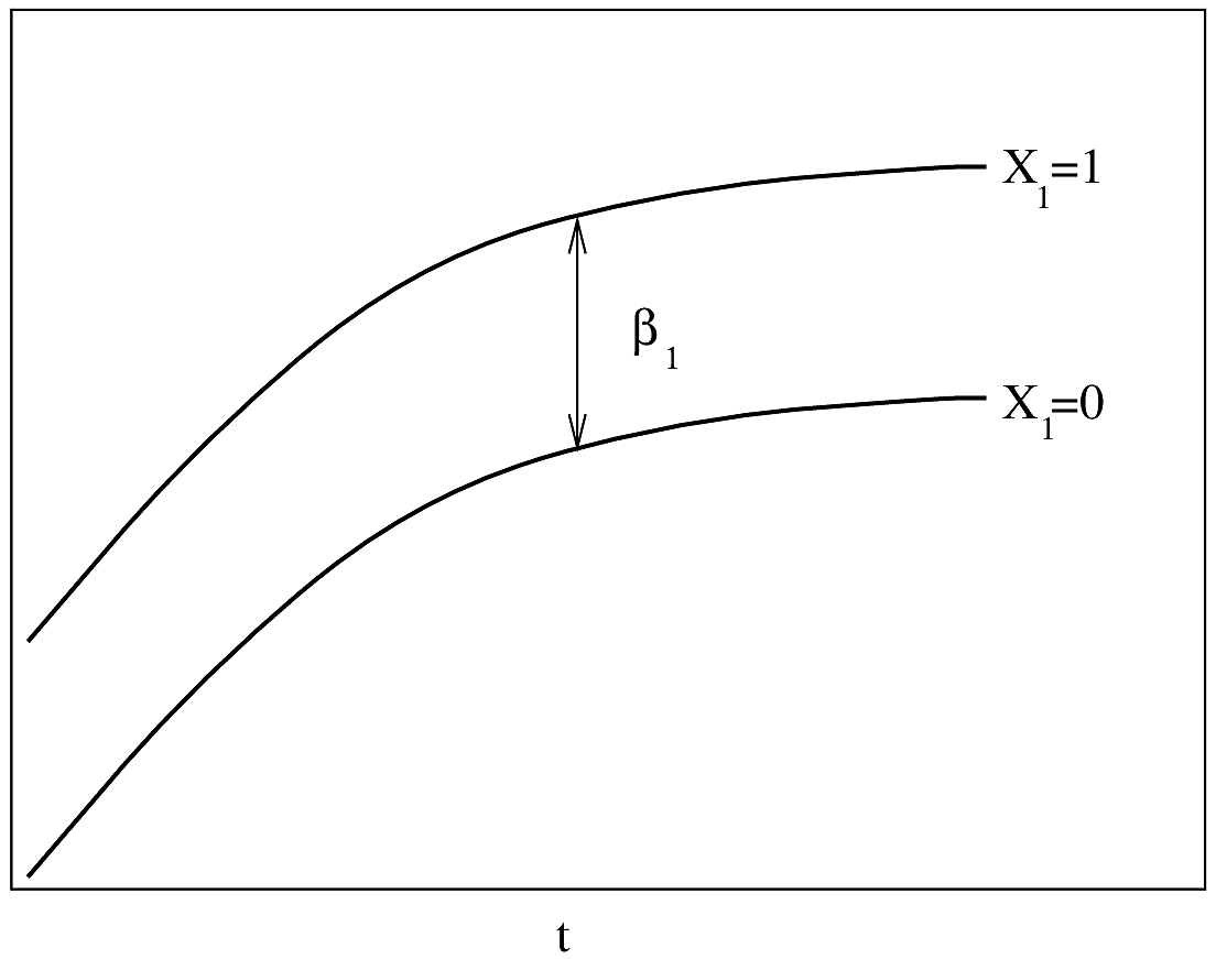
\[\begin{array}{ccc} \Lambda(t|X) &=& \Lambda(t) \exp(X\beta) \nonumber \\ S(t|X) &=& \exp[-\Lambda(t)\exp(X\beta)] = \exp[-\Lambda(t)]^{\exp(X\beta)} \end{array}\]\[ S(t|X) = S(t)^{\exp(X\beta)} , \]
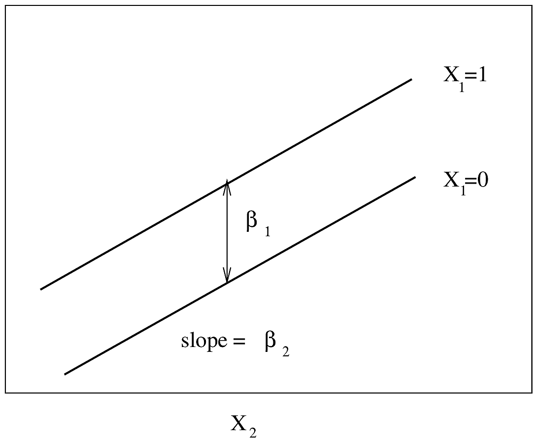
Assumptions:
Here \(\exp(\beta_{1})\) is the \(X_{1}=1:X_{1}=0\) hazard ratio.
\[ \lambda(t|X_{1}) = \lambda(t)\exp(\beta_{1}X) \]
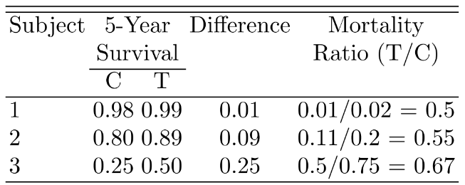
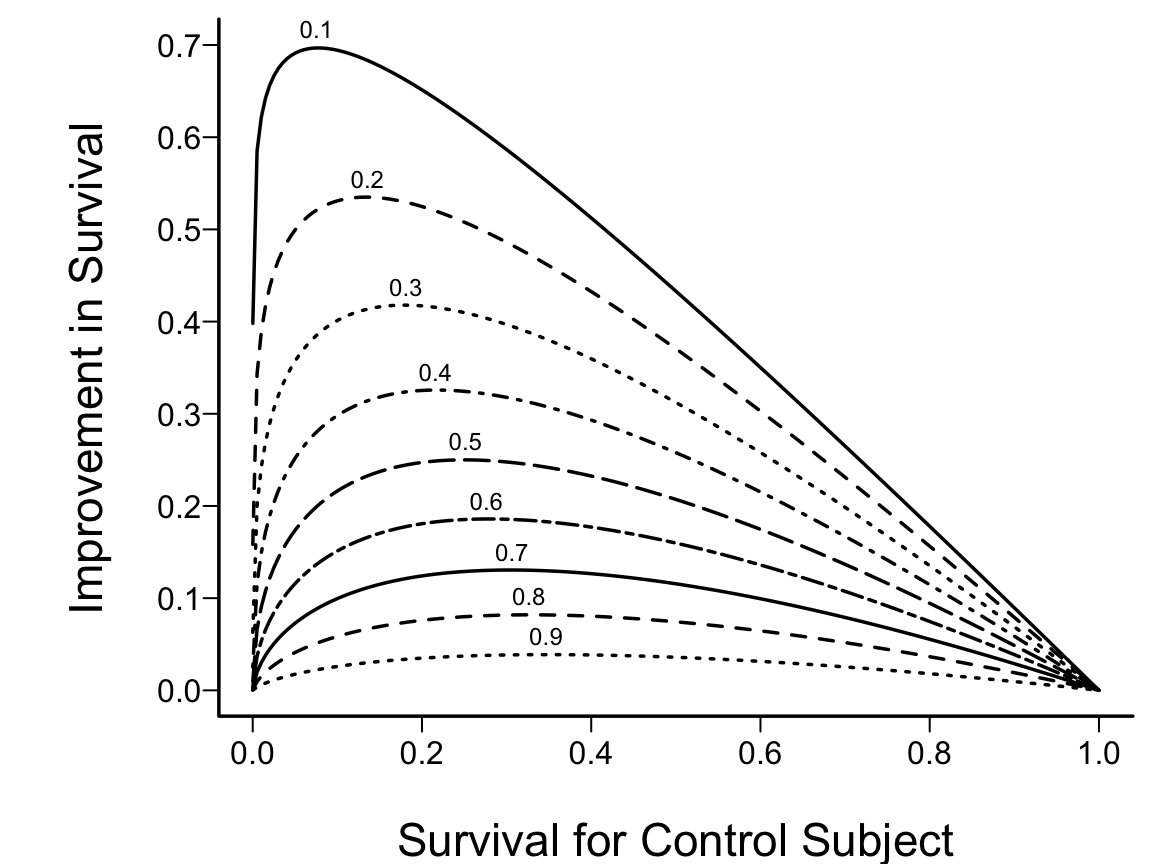
\(S_{T}=S_{C}^{0.5}\)
spar(bty='l')
plot(0, 0, type="n", xlab="Survival for Control Subject",
     ylab="Improvement in Survival",
     xlim=c(0,1), ylim=c(0,.7))
i <- 0
hr <- seq(.1, .9, by=.1)
for(h in hr) {
  i <- i + 1
  p <- seq(.0001, .9999, length=200)
  p2 <- p^h
  d <- p2 - p
  lines(p, d, lty=i)
  maxd <- max(d)
  smax <- p[d==maxd]
  text(smax,maxd+.02, format(h), cex=.6)
}
\[ T_{0.5}|X=\{\log 2 / [\alpha \exp(X\beta)]\}^{1/\gamma} . \]
For numerical reasons, re-write:
\[\begin{array}{ccc} S(t|X) &=& \exp(-\Lambda(t|X)) , {\rm\ \ \ where} \nonumber \\ \Lambda(t|X) &=& \exp(\gamma \log t + X\beta) \end{array} \tag{18.1}\]
See also spline hazard models Kooperberg et al. (1995) and the generalized gamma distribution (Cox et al., 2007).
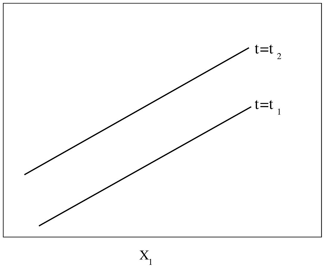
If \(\lambda(t)\) is Weibull, the two curves will be linear if \(\log t\) is plotted instead of \(t\) on the \(x\)-axis.
\[S(t|X) = \psi(\frac{\log(t)-X\beta}{\sigma}) \tag{18.2}\]
\[\begin{array}{ccc} \frac{\log(T)-X\beta}{\sigma} &\sim& \psi \\ \log(T) = X\beta + \sigma\epsilon \\ \epsilon \sim \psi \end{array}\]\[ \psi^{-1}(S(t|X)) = \frac{\log(t)-X\beta}{\sigma} \tag{18.3}\]
Letting \(\epsilon \sim \psi\)
\[ \log(T) = X\beta + \sigma\epsilon \]
Check that residuals \(\log(T)-X\hat{\beta} \sim \psi\) (within scale factor). The assumptions of the AFT model are thus
1-unit change in \(X_{j} = \beta_{j}\) change in \(\log T\), or increase \(T\) by factor of \(\exp(\beta_{j})\).
Median survival time:
\[ T_{0.5}|X = \exp(X\beta + \sigma \psi^{-1}(0.5)) \]
\[ S(t|X) = 1 - \Phi(\frac{\log(t)-X\beta}{\sigma}), \]
\[ S(t|X) = [1 + \exp(\frac{\log(t) - X\beta}{\sigma})]^{-1}. \]
Works better if \(\sigma\) parameterized as \(\exp(\delta)\).
\[\begin{array}{ccc} \hat{S}(t|X) &=& \psi(\frac{\log(t)-X\hat{\beta}}{\hat{\sigma}}) \nonumber \\ \hat{T}_{0.5}|X &=& \exp[X\hat{\beta} + \hat{\sigma} \psi^{-1}(0.5)]. \end{array}\]Normal and logistic: \(\hat{T}_{0.5}|X = \exp(X\hat{\beta})\)
\[ \psi(\frac{\log(t)-X\hat{\beta}}{\hat{\sigma}}\pm z_{1-\alpha/2}\times s) \]
For an AFT model, standardized residuals are simply
\[ r = (\log(T)-X\hat{\beta})/\sigma \tag{18.4}\]
When \(T\) is right-censored, \(r\) is right-censored.

| Group 1 | 143 | 164 | 188 | 188 | 190 | 192 | 206 | 209 | 213 | 216 |
| 220 | 227 | 230 | 234 | 246 | 265 | 304 | 216\(^{+}\) | 244\(^{+}\) | ||
| Group 2 | 142 | 156 | 163 | 198 | 205 | 232 | 232 | 233 | 233 | 233 |
| 233 | 239 | 240 | 261 | 280 | 280 | 296 | 296 | 323 | 204\(^{+}\) | |
| 344\(^{+}\) |
spar(mfrow=c(2,2), top=1, bot=2, mgp=c(2.75, .365, 0))
getHdata(kprats)
kprats$group <- factor(kprats$group, 0:1, c('Group 1', 'Group 2'))
dd <- datadist(kprats); options(datadist="dd")
S <- with(kprats, Surv(t, death))
f <- npsurv(S ~ group, type="fleming", data=kprats)
survplot(f, n.risk=TRUE, conf='none',
         label.curves=list(keys='lines'), levels.only=TRUE)
title(sub="Nonparametric estimates", adj=0, cex=.7)
# Check fits of Weibull, log-logistic, log-normal
xl <- c(4.8, 5.9)
survplot(f, loglog=TRUE, logt=TRUE, conf="none", xlim=xl,
         label.curves=list(keys='lines'), levels.only=TRUE)
title(sub="Weibull (extreme value)", adj=0, cex=.7)
survplot(f, fun=function(y)log(y/(1-y)), ylab="logit S(t)",
         logt=TRUE, conf="none", xlim=xl,
         label.curves=list(keys='lines'), levels.only=TRUE)
title(sub="Log-logistic", adj=0, cex=.7)
survplot(f, fun=qnorm, ylab="Inverse Normal S(t)",
         logt=TRUE, conf="none",
         xlim=xl,cex.label=.7,
         label.curves=list(keys='lines'), levels.only=TRUE)
title(sub="Log-normal", adj=0, cex=.7)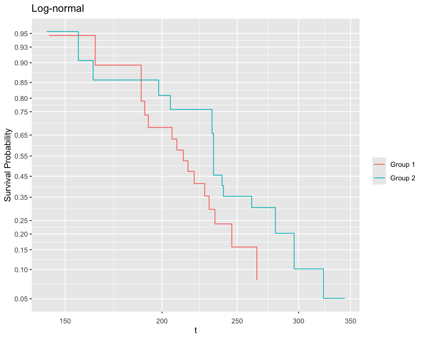
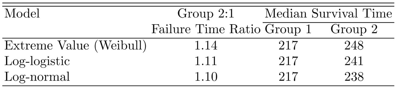
Fit Weibull (in aft form), log-logistic, and log-normal models.
fw <- psm(S ~ group, data=kprats, dist='weibull')
fl <- psm(S ~ group, data=kprats, dist='loglogistic',
          y=TRUE)
fn <- psm(S ~ group, data=kprats, dist='lognormal')
bld <- function(x) knitr::asis_output(paste0('**', x, '** :\n\n'))
bld('Weibull default form')
Weibull default form :
latex(fw)\[[c]=1~\mathrm{if~subject~is~in~group}~c,~0~\mathrm{otherwise}\]
bld('Weibull PH form')Weibull PH form :
latex(pphsm(fw))\[[c]=1~\mathrm{if~subject~is~in~group}~c,~0~\mathrm{otherwise}\]
bld('Log-logistic')Log-logistic :
latex(fl)\[[c]=1~\mathrm{if~subject~is~in~group}~c,~0~\mathrm{otherwise}\]
bld('Log-normal')Log-normal :
latex(fn)\[[c]=1~\mathrm{if~subject~is~in~group}~c,~0~\mathrm{otherwise}\]
survplot(f, conf.int=FALSE,
         levels.only=TRUE, label.curves=list(keys='lines'))
survplot(fl, add=TRUE, label.curves=FALSE, conf.int=FALSE)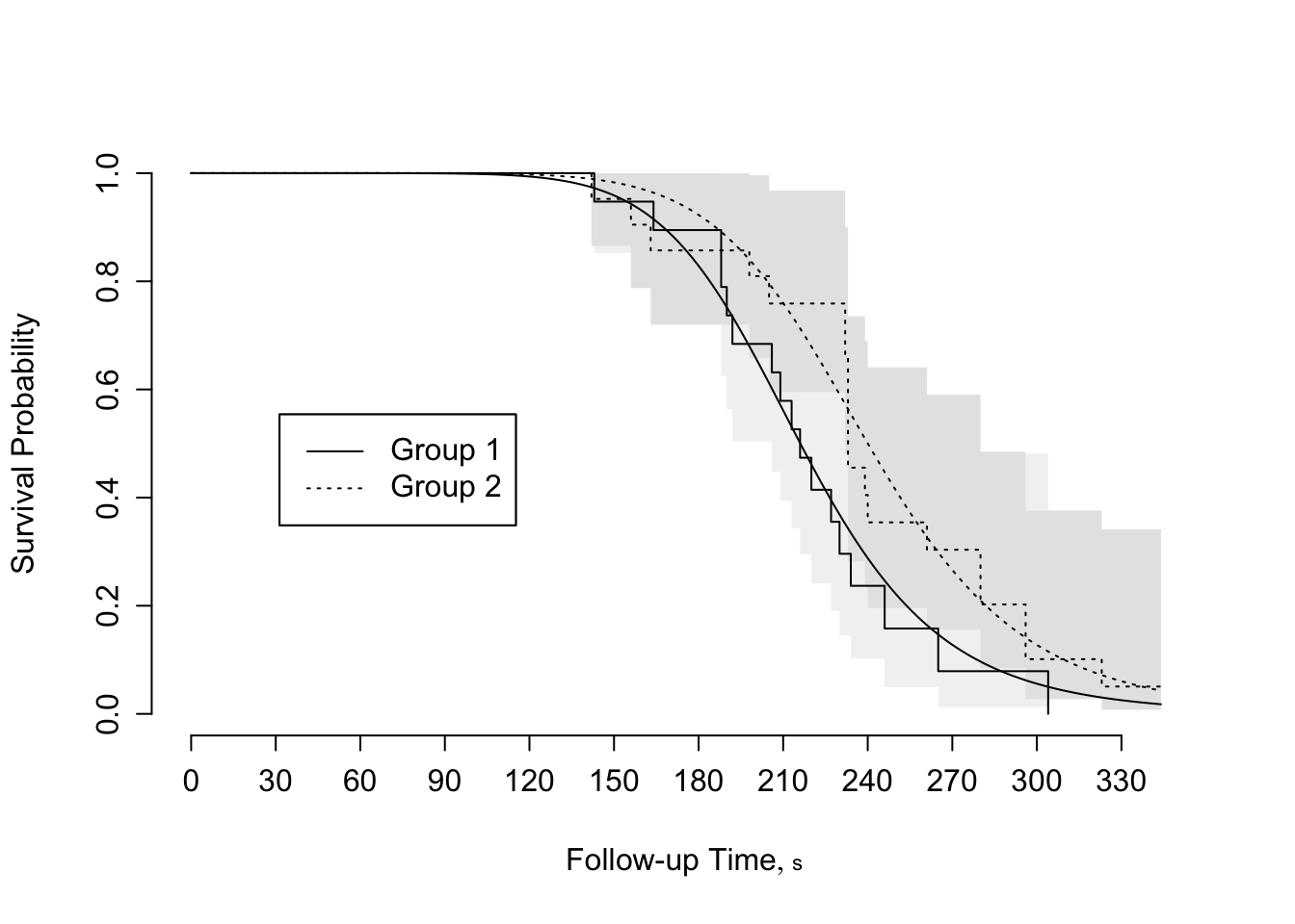
r <- resid(fl, 'cens')
survplot(npsurv(r ~ group, data=kprats),
         conf='none', xlab='Residual',
         label.curves=list(keys='lines'), levels.only=TRUE)
survplot(npsurv(r ~ 1), conf='none', add=TRUE, col='red')
lines(r, lwd=1, col='blue') 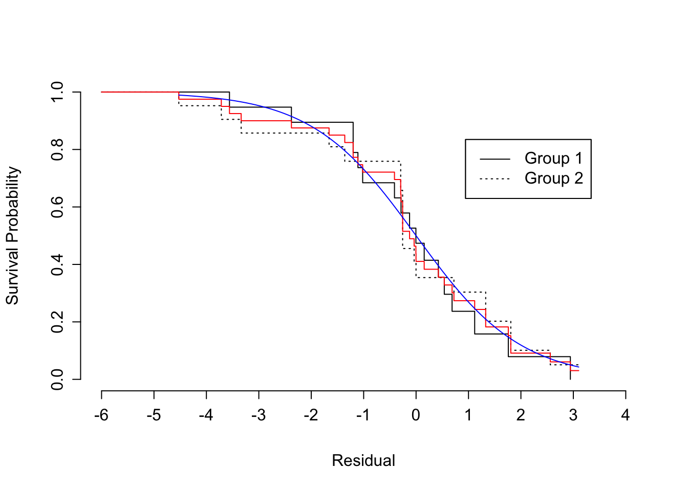
Derive R code for median, mean, hazard, survival functions
med   <- Quantile(fl)
med
function (q = 0.5, lp = NULL, parms = -2.15437773933124)
{
names(parms) <- NULL
f <- function(lp, q, parms) lp + exp(parms) * logb(q/(1 -
q))
names(q) <- format(q)
drop(exp(outer(lp, q, FUN = f, parms = parms)))
}
<environment: namespace:rms>meant <- Mean(fl)
meantfunction (lp = NULL, parms = -2.15437773933124)
{
names(parms) <- NULL
if (exp(parms) > 1)
rep(Inf, length(lp))
else exp(lp) * pi * exp(parms)/sin(pi * exp(parms))
}
<environment: namespace:rms>haz <- Hazard(fl)
hazfunction (times = NA, lp = NULL, parms = -2.15437773933124)
{
t.trans <- logb(times)
t.deriv <- 1/times
scale <- exp(parms)
names(t.trans) <- format(times)
t.deriv/scale/(1 + exp(-(t.trans - lp)/scale))
}
<environment: namespace:rms>surv <- Survival(fl)
survfunction (times = NULL, lp = NULL, parms = -2.15437773933124)
{
1/(1 + exp((logb(times) - lp)/exp(parms)))
}
<environment: namespace:rms>Show fitted hazard function from log-logistic, and add median survival time to graph
spar(ps=9,top=1,bot=1,left=1,mgp=c(2.75,.365,0))
# Plot estimated hazard functions and add median
# survival times to graph
survplot(fl, group, what="hazard")
# Compute median survival time
m <- med(lp=predict(fl,
           data.frame(group=levels(kprats$group))))
m
1 2
216.0857 240.0328 med(lp=range(fl$linear.predictors))[1] 216.0857 240.0328m <- format(m, digits=3)
text(68, .02, paste("Group 1 median: ", m[1],"\n",
"Group 2 median: ", m[2], sep=""))
# Compute survival probability at 210 days
xbeta <- predict(fl,
data.frame(group=c("Group 1","Group 2")))
surv(210, xbeta) 1 2
0.5612718 0.7599776 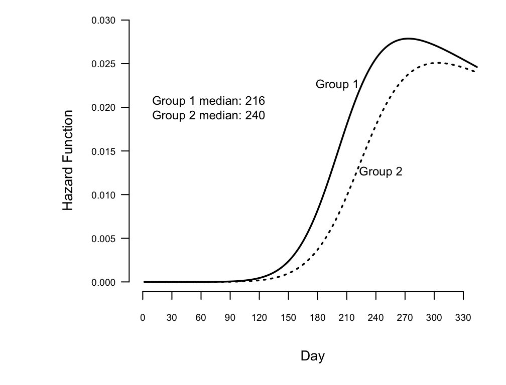
loess smooth of \(F(T | X) - 0.5 F(C | X)\) against \(X
\hat{\beta}\) or \(\frac{2 F(T | X)}{F(C | X)}\) vs. \(X \hat{\beta}\) if \(C\) is knownSee the val.surv function in the rms package.
R Functionssurvival package: survreg for Weibull, log-normal, log-logistic, etc.rms package: psm front-end for survregrstpm2 package: cran.r-project.org/web/packages/rstpm2 which has more general AFT modelsR packages: