• Do you wonder why we have so many special cases in statistics that require seemingly different methods?
  • time to first event
  • recurrent events
  • recurrent events with an absorbing state
  • cure models (two absorbing states)
  • competing risks

• More special cases
  • Wilcoxon, Kruskal-Wallis, logrank tests
  • zero inflation adaptations of Poisson and negative binomial models
  • longitudinal data analysis

• \(\Pr(Y \geq y | X) = \mathrm{expit}(\alpha_{y} + X\beta)\)
• \(Y\)-transformation invariant, does not use \(Y\) spacings
• Handles arbitrarily heavy ties or continuous \(Y\), bi-modality, …
• Direct competitor of the linear model

• Random intercepts
  • massive lack of fit for correlation structure
    • implies there is interest in individual pt-level outcomes vs. group level (treatment level)
    • absorbing states destroy the correlation pattern
    • typically assumes that > 6 observations per patient do not increase power

• Random intercepts and slopes
  • more flexible correlation structure but still may not fit
    • too many parameters to estimate
  • can’t have absorbing states
• Markov models
  • most flexible, fastest, easiest to program
    • trivial to implement with ML (until you want state occupancy probabilities)

• Markov models apply to all \(Y\)
  • binary
  • unordered categorical
  • ordinal categorical
  • ordinal continuous
  • ordinal mixed continuous and categorical
  • continuous
  • left, right, and interval censored
  • require unconditioning on previous \(Y\) to get marginal distributions

• Current state depends only on covariates, previous state
• Let measurement times be \(t_{1}, t_{2}, \dots, t_{m}\), and the measurement for a patient at time \(t\) be denoted \(Y(t)\) \[\Pr(Y(t_{i}) \geq y | X, Y(t_{i-1})) =\] \[\mathrm{expit}(\alpha_{y} + X\beta + g(Y(t_{i-1}), t_{i}))\]

• Time to terminating event
  • transition probability = discrete hazard rate
  • OR \(\approx\) HR when time intervals small
  • easily handles time-dependent covariates, left-truncation
• Recurrent binary events
• Recurrent binary events + a terminal event

• Competing risks
  • death explicitly handled as a bad outcome
  • easier to interpret than competing risk models
• Serial current status data
  • events of different severities
  • no need to judge whether an early heart attack is worse than a late death
• Missing data and interval-censored \(Y\)

• Standard longitudinal continuous \(Y\)
• Longitudinal continuous or ordinal \(Y\) interrupted by clinical events
• Easily handles multiple absorbing states
• Serial correlation: condition on previous outcome
• Random intercepts (compound symmetry correlation): condition on average of all previous outcomes

• 0=alive 1=dead
  • censored at 3w: 000
  • death at 2w: 01
• 0=at home 1=hospitalized 2=MI 3=dead
  • hospitalized at 3w, rehosp at 7w, MI at 8w & stays in hosp, f/u ends at 10w: 0010001211

• 0-6 QOL excellent–poor, 7=MI 8=stroke 9=dead
  • QOL varies, not assessed in 3w but pt event free, stroke at 8w, death 9w: 12[0-6]334589
  • MI status unknown at 7w: 12[0-6]334[5,7]89
• Can make first 200 levels be a continuous response variable and the remaining values represent clinical event overrides

• For equal time spacing:
  \(\Pr(Y(t)=y | X) =\)
  \(\sum_{j=1}^{k}\Pr(Y(t)=y | X, Y(t-1) = j) \times\)
  \(\Pr(Y(t-1) = j | X)\)
• Use this recursively
• Yields a semiparametric unconditional (except for \(X\)) distribution of \(Y\) at each \(t\) (SOPs)
• soprobMarkovOrd* functions in the R Hmisc package make this easy for frequentist and Bayesian models

• Transition odds ratios (original parameters)
• Prior state and covariate-specific transition probabilities
• State occupancy probabilities (SOPs; marginalize over time)
• Covariate-specific SOPs
  • \(\Pr(\)stroke in week 4 or death in or before week 4\()\); \(\Pr(\)stroke and alive\()\)

• Time in state \(Y=y\) (like RMST)
• Time in states \(Y \geq y\) (e.g., mean time unwell)
• Differences in mean time in state between treatments
• Continuous \(Y\) example: mean time with SBP < 130mmHg
  • Nice way to handle treatment \(\times\) time interaction
  • No categorization of SBP

FA Simader et al (2024): Symptoms as a predictor of the placebo-controlled efficacy of PCI in stable coronary artery disease. JACC 84: 13-24.

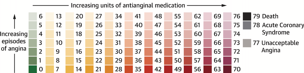
• Daily angina frequencies
• Y = ordinal scale
  • Angina frequencies magnified by # units of anti-anginal meds required to control angina
  • Clinical event overrides at top of scale
  • Graphic design by Matthew Shun-Shin, Imperial College London

• Detailed case study with complete R code at hbiostat.org/rmsc/markov
• Statistics in Medicine tutorial

• Allows effect of Tx to vary over outcome categories
• Example: Tx may affect mortality differently than how it affects function/Sx
• Bayesian prior can specify limits on the amount of borrowing of Tx effects across outcomes
• Example Bayesian posterior prob.: probability that Tx affects death by \(> 1.5\times\) effect on function
• See fharrell.com/post/yborrow

• Surrogate endpoint: an endpoint affected by Tx if and only if the Tx affects the gold standard (GS) endpoint
• Surrogates are used to mirror and give an early preview to the GS
• Very difficult to establish surrogacy, and it is unreasonable to assume Pr(surrogacy) is 0 or 1
• If you think of this as a multiple imputation problem (using surrogate to impute the GS), \(N\) for an RCT based on a surrogate may be greater than \(N\) needed for GS!

Instead:

• Include the (lower powered) GS as part of an ordinal outcome
• Construct an ordinal outcome built on consensus about severities of outcomes
• Decide on how much information you want to borrow across endpoints
• I.e., how does a posterior distribution for Tx effect on nonfatal endpoint help build the posterior for the effect on GS

• hbiostat.org/ordinal
• hbiostat.org/endpoint
• fharrell.com/talk/cmstat