Positive errors: OK by definition if analysis prior = reviewer’s
prior
Bayesian power affected by prior but dominated by \(N\) and uncertainty in MCID
Simulations compute P(correct decision) when there is a disagreement
in priors
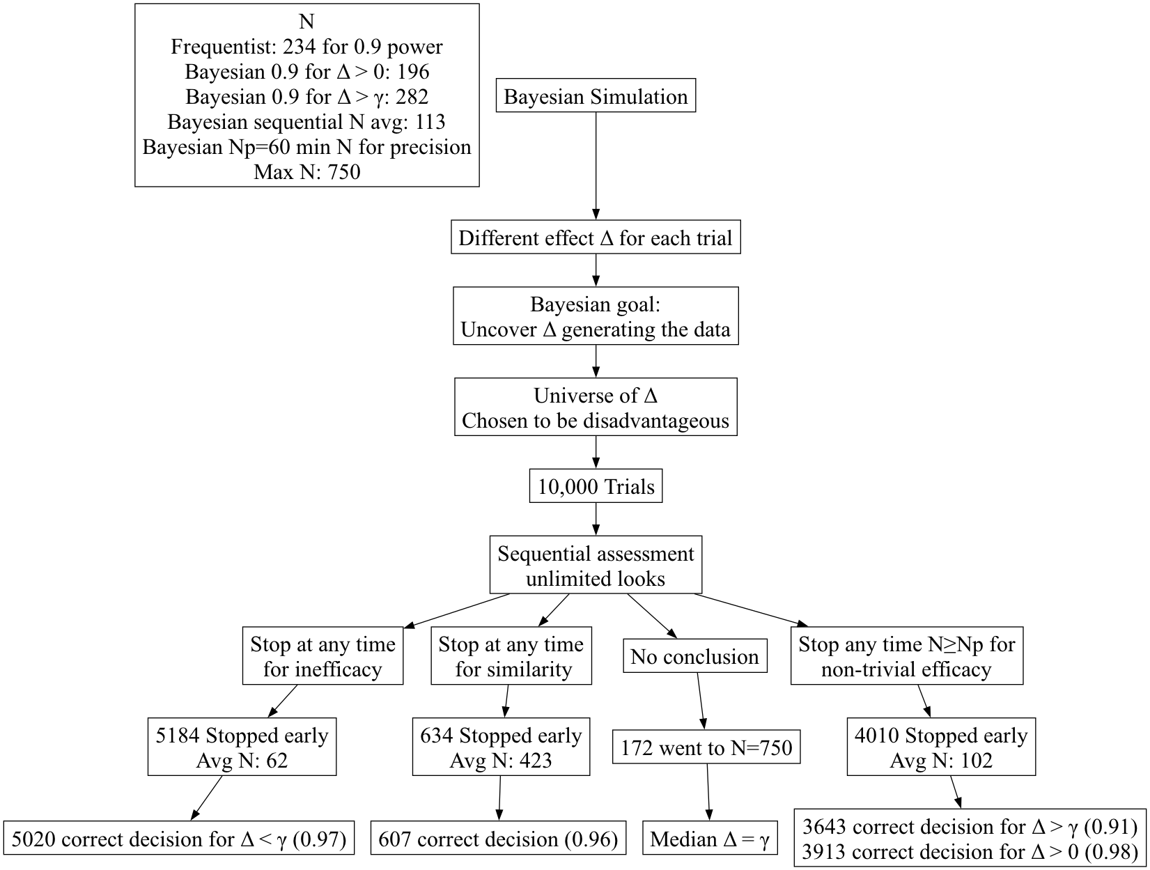
Simulation setup: simulate 1000 RCTs with 1000 values of \(\Delta\)
Bayes’ goal: uncover hidden truths behind the data generating
mechanism relying only on observables
Of those 1000 in which a certain decision was made, count how often
the decision was correct, i.e.,
Subset the trials to those in which decision \(D\) was made
Reveal the \(\Delta\) generating
the data in those trials
Check how often \(\Delta\) was in
the interval corresponding to \(D\)
Accuracy is a post-data consideration
Is conditional on the data and the decision, not \(\Delta\)
Simulation
Design Reveals Dramatic Differences Between Paradigms
Frequentist simulations couldn’t be more different
and have little to do with data-based decision making
Simulate 1000 RCTs in which the treatment is irrelevant (\(\Delta=0\))
Compute a test statistic and \(p\)-value
Count how often \(p\)<0.05
Likewise for a single all-too-arbitrary positive treatment
effect
Multiplicities exist because \(p\)
= P(data extreme) instead of P(\(\Delta\)) more chances for data to be
extreme with more data looks
Extreme
Importance of Goal-Driven Sequential Designs
Sample size calculations are voodoo
MCID is gamed and should be recognized as having uncertainty
Majority of RCTs are equivocal
Equivocal studies on average could perhaps have been stopped for
futility \(\frac{1}{3}\) of the way
through
Quiz: if the current treatment effect is harmful, how far along in
trial recruitment can you be for you to still have a good chance of
ultimately showing treatment benefit?
Bayes
Needs No Multiplicity Adjustment for \(\infty\) Data Looks
Consider a posterior prob (PP) computed at the study end
Interim analyses use the same construction of PP and same prior so
must also be valid
Early PP are merely made obsolete by later data
P(decision error) independent of stopping rules
Expected sample size is minimized by maximizing # looks
Two-Treatment
Parallel-Group Efficacy Design Comparing Two Means, Known \(\sigma=1\)
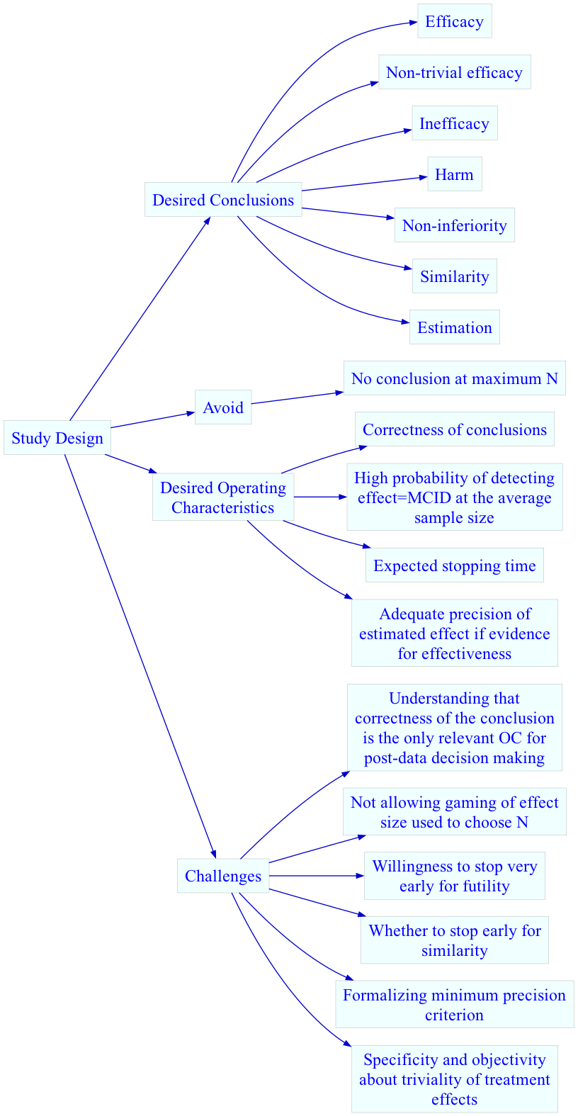
Goals
Maximize the probability of making the right decision, with 4
decisions possible (efficacy, similarity, inefficacy, not possible to
draw any conclusion with available resources)
Minimize the probability of an inconclusive result at study end
Minimize the expected sample size
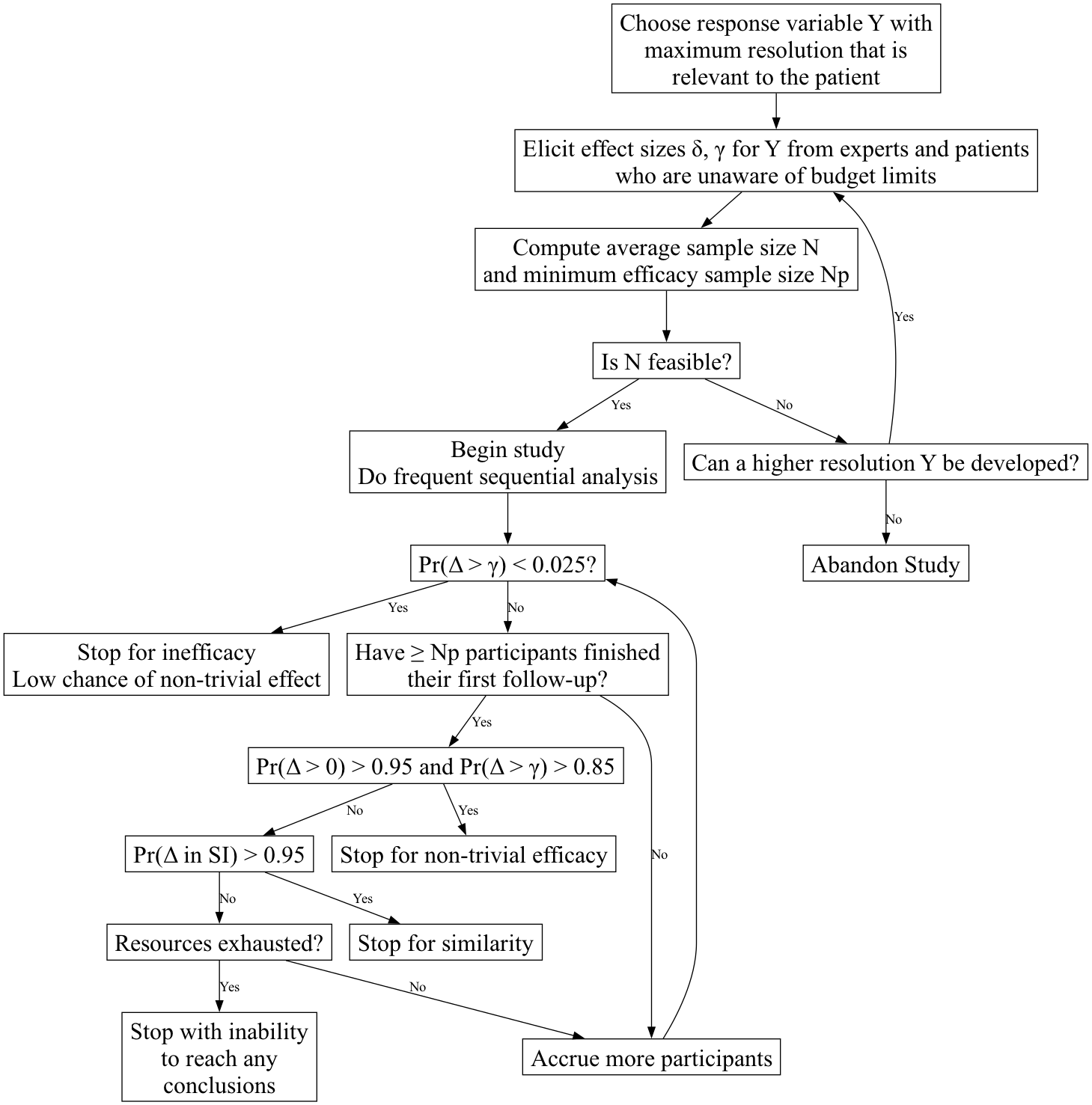
Stop as early as possible if there is a very high probability that
the treatment’s effect is trivial or worse, even if the magnitude of the
effect cannot be estimated with any precision
If stopping early for non-trivial efficacy, make sure that the
sample size provides at least crude precision of the effect estimate
Do this by not making the first efficacy look until the lowest
sample size for which at least crude precision of the treatment effect
is attained
Avoid gaming the effect size used in a power calculation
Recognize that traditional sample sizes are arbitrary and require
too many assumptions
Recognize that what appears to be a study extension to one person
will appear to be an interim analysis to another who doesn’t need to do
a sample size calculation
Build clinical significance into the quantification of evidence for
efficacy
Definitions
\(\Delta\): true treatment effect
being estimated
\(\delta\): minimum clinically
important \(\Delta\)
\(\gamma\): minimum detectable
\(\Delta\) (threshold for non-trivial
treatment effect, e.g. \(\frac{1}{3}\delta\))
SI: similarity interval for \(\Delta\), e.g., \([-\frac{1}{2}\delta,
\frac{1}{2}\delta]\)
\(N\): average sample size, used
for initial resource planning. This is an estimate of the ultimate
sample size based on assuming \(\Delta =
\delta\). \(N\) is computed to
achieve a Bayesian power of 0.9 for efficacy, i.e., achieving a 0.9
probability at a fixed sample size that the probability of any efficacy
exceeds 0.95 while the probability of non-trivial efficacy exceeds 0.85,
i.e., \(\Pr(\Delta > 0) > 0.95\)
and \(\Pr(\Delta > \gamma) >
0.85\).
More than one \(N\) can be
computed, e.g., \(N\) such that if
\(\Delta = \gamma\) there is ever a
high probability of stopping for inefficacy
\(N_p\): minimum sample size for
first efficacy assessment, based on required minimum precision of
estimate of \(\Delta\)
Probability cutoffs are examples
This design does not require a separate futility analysis, as
inefficacy subsumes futility
Below, “higher resolution Y” can come from breaking ties in the
outcome variable (making it more continuous), adding longitudinal
assessments, or extending follow-up
Simulated
Performance of Frequentist Group Sequential Design
Hwang-Shih-Decani bounds with \(\gamma =
-4\) for overall \(\alpha=0.05\)
one-sided
gsDesign R package
Least conservative bounds such that final nominal \(\alpha\) is close to overall \(\alpha\)
Test for non-trivial efficacy at N=60, 65, 70, … 750
Tests for inefficacy/trivial efficacy and similarity at N=5, 10, 15,
…, 750
Test for similarity: group sequential version of rejecting two
one-sided tests at \(\alpha=0.025\) to
coincide with Bayesian probability of 0.95
Other than initial part of efficacy boundary being non-monotonic due
to minimum efficacy sample size of N=60 per group, bounds for efficacy
and inefficacy are negatives of each other
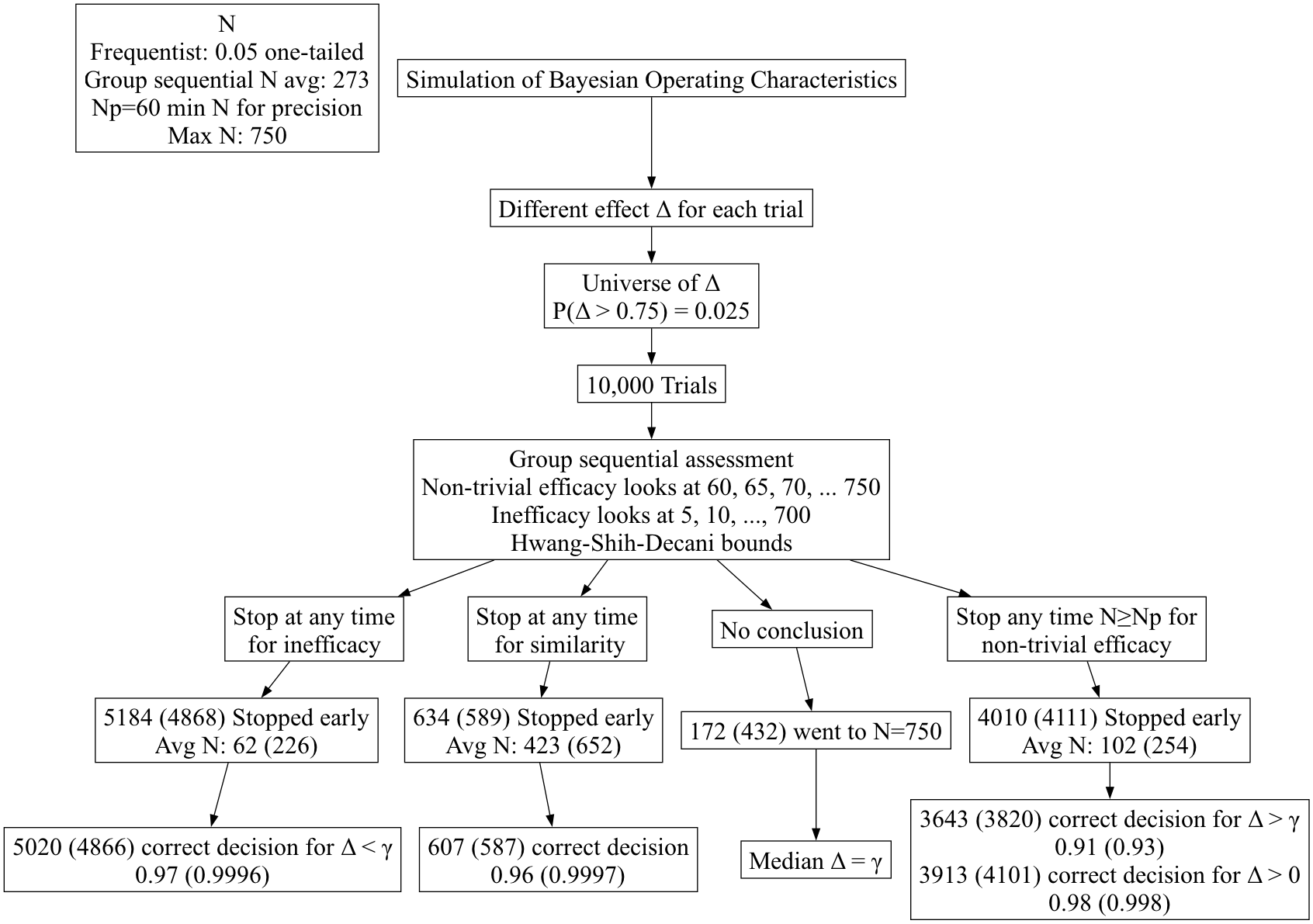
Simulated Bayesian operating characteristics of frequentist
procedure (correctness of decisions & expected sample sizes to reach
decisions)
Frequentist results are in ()
Summary of Group Sequential
Results
Group sequential bounds are seen as ultra-conservative by a
Bayesian
Due to their conservatism, when exceeding a group sequential
boundary one may be confident in the decision
The problem is that the frequentist procedure takes far too long to
reach a decision, with more than double the expected sample sizes
Group sequential methods are portrayed as protecting against early
harm but this is misleading because of their ultra-low power at early
looks
The Bayesian procedure is extremely reliable even though it was
penalized for a prior mismatch
Summary
Disciplined choices of MCID, outcomes, and trivial effects margins
\(\uparrow\) likelihood of study
success or abandoning futile studies before any $ spent
It’s best to not have a sample size calculation, especially if
assuming what we’re trying to learn from the study
Sequential designs can easily have multiple explicit clinical goals
in the Bayesian framework
They can greatly speed up research
Bayesian OCs can be very impressive even with conflicting
priors
Frequentist group sequential designs take much longer to reach both
inefficacy (especially) and efficacy decisions