How to Do Bad Biomarker Research
Prelude
Biomarker Uncertainty Principle: A molecular signature derived from high-dimensional data can be either parsimonious or predictive, but not both.
We have more data than ever, more good data than ever, a lower proportion of data that are good, a lack of strategic thinking about what data are needed to answer questions of interest, sub-optimal analysis of data, and an occasional tendency to do research that should not be done.
Fundamental Principles of Statistics
Before discussing how much of biomarker research has gone wrong from a methodologic viewpoint, it’s useful to recall statistical principles that are used to guide good research.
- Use methods grounded in theory or extensive simulation
- Understand uncertainty
- Design experiments to maximize information
- Verify that the sample size will support the intended analyses, or pre-specify a simpler analysis for which the sample size is adequate; live within the confines of the information content of the data
- Use all information in data during analysis
- Use discovery and estimation procedures not likely to claim that noise is signal
- Strive for optimal quantification of evidence about effects
- Give decision makers the inputs other than the utility function that optimize decisions
- Present information in ways that are intuitive, maximize information content, and are correctly perceived
Example of What Can Go Wrong
A paper in JAMA Psychiatry (McGrath et al. (2013)) about a new neuroimaging biomarker in depression typifies how violations of some of the above principles lead to findings that are very unlikely to either be replicated or to improve clinical practice. It also illustrates how poor understanding of research methodology by the media leads to hype.
Consider how the New York Times reported the findings.

The Times article claimed that we now know whether to treat a specific depressed patient with drug therapy or behavioral therapy if a certain imaging study was done. This finding rests on assessment of interactions of imaging results with treatment in a randomized trial.
To be able to estimate differential treatment benefit requires either huge numbers of patients or the use of a high-precision patient outcome. Neither of these is the case in the authors’ research. The authors based the analysis of treatment response on the Hamilton Depression Rating Scale (HDRS), which is commonly used in depression drug studies. The analysis of a large number of candidate PET image markers against the difference in HDRS achieved by each treatment would not lead to a very reliable result with the starting sample size of 82 randomized patients. But the authors made things far worse by engaging in dichotomania, defining an arbitrary “remission” as the patient achieving HDRS of 7 or less at both weeks 10 and 12 of treatment. Besides making the analysis arbitrary (the cutoff of 7 is not justified by any known data), dichotomization of HDRS results in a huge loss in precision and power. So the investigators began with an ordinal response, then lost much of the information in HDRS by dichotomization. This loses information about the severity of depression and misses close calls around the HDRS=7 threshold. It treats patients with HDRS=7 and 8 as more different than patients with HDRS=8 and HDRS=25. No claim of differential treatment effect should be believed unless a dose-response relationship for the interacting factor can be demonstrated. The “dumbing-down” of HDRS reduces the effective sample size and makes the results highly depend on the cutoff of 7. Lower effective size means decreased reproducibility.
The simplest question that can possibly be answered using binary HDRS involves estimating the proportion of responders in a single treatment group. The sample size needed to estimate this simple proportion to within a 0.05 margin of error with 0.95 confidence is is n=384. The corresponding sample size for comparing two proportions for equal sample sizes n=768 in each group. In the best possible (balanced) case the sample size needed to estimate a differential treatment effect (interaction affect) is four times this.
The idea of estimating differential treatment effects over a large number of image characteristics with a sample size n=82 that is inadequate for estimating a single proportion is preposterous. Yet the investigators claimed to learn from complex brain imaging analysis on 6 non-responders to drug and 9 non-responders to behavioral therapy which depression patients would have better outcomes under drug therapy vs. behavioral therapy.
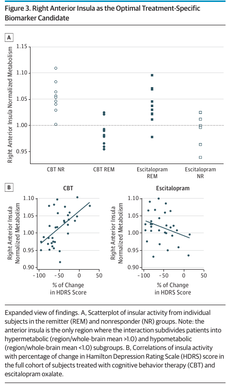
The cherry-picked right anterior insula was labeled as the optimal treatment-specific biomarker candidate (see their Figure 3 below). It is very unlikely to be reproduced.
A key result of McGrath et al. (2013) is given in their Table 1, reproduced below.
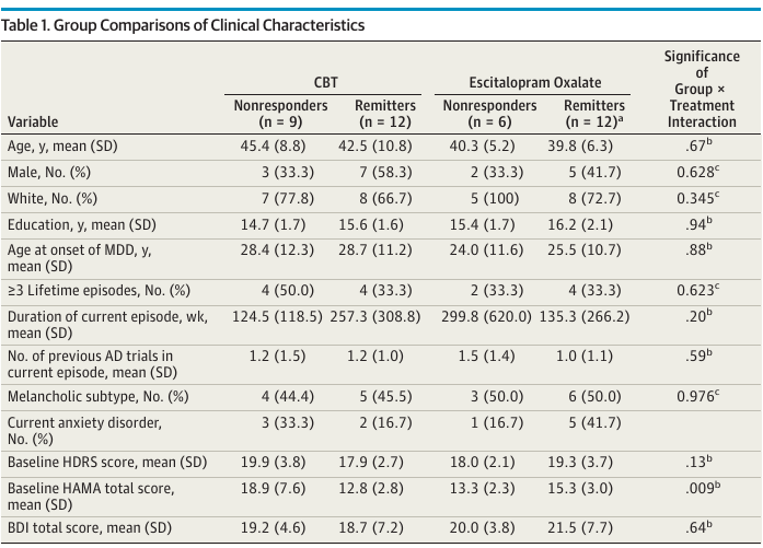
An interesting finding in the next-to-last row of this table. There was evidence for an interaction between treatment and the baseline HAMA total score, which is an anxiety score. The direction of the interaction is such that patients with higher anxiety levels at baseline did worse with behavioral therapy. This involves a low-tech metric but has some face validity and is undoubtedly stronger and more clinically relevant than any of the authors’ findings from brain imaging, if validated. The authors’ emphasis of imaging results over anxiety levels is puzzling, especially in view of fact that the the clinical variable analyses involved less multiplicity problems than the analysis of imaging parameters.
Note: The authors attempted to replicate their 2013 findings in 2021 and were unable to do so.
Analysis That Should Have Been Done
The analysis should use full information in the data and not use an arbitrary information-losing responder analysis. The bootstrap should be used to fully expose the difficulty of the task of identifying image markers that are predictive of differential treatment effect. This is related to the likelihood that the results will be replicated in other datasets.
Here are some steps that would accomplish the biomarker identification goal or would demonstrate the futility of such an analysis. The procedure outlined recognizes that the biomarker identification goal is at its heart a ranking and selection problem.
- Keep HDRS as an ordinal variable with no binning.
- Use a proportional odds ordinal logistic model to predict final HDRS adjusted for treatment and a flexible spline function of baseline HDRS.
- Similar to what was done in the
Bootstrap Ranking Examplesection below, bootstrap all the following steps so that valid confidence intervals on ranks of marker importance may be computed. Take for example 1000 samples with replacement from the original dataset. - For each bootstrap sample and for each candidate image marker, augment the proportional odds model to add each marker and its interaction with treatment one-at-a-time. All candidate markers must be considered (no cherry picking).
- For each marker compute the partial \(\chi^2\) statistic for its interaction with treatment.
- Over all candidate markers rank their partial \(\chi^2\).
- Separately from each set of 1000 bootstrap per-marker importance ranks for each candidate marker, compute a bootstrap confidence interval for the rank.
The likely result is that the apparent “winner” will have a confidence interval that merely excludes it as being one of the biggest losers. The sample size would likely have to be \(\geq 10\times\) as large for the confidence intervals to be narrow enough for us to have confidence in the “winner”. The likelihood that the apparent winner is the actual winner in the long run is close to zero.
Dichotomania and Discarding Information
What Kinds of True Thresholds Exist?
Natura non facit saltus (Nature does not make jumps) — Gottfried Wilhelm Leibniz
With much of biomarker research relying on dichotomization of continuous phenomena, let’s pause to realize that such analyses assume the existence of discontinuities in nature that don’t exist. The non-existence of such discontinuities in biomarker-outcome relationships is a key reason that cutpoints “found” in one dataset do not replicate in other datasets. They didn’t exist in the first dataset to begin with, but were found by data torture. Almost all continuous variables in nature operate in a smooth (but usually nonlinear) fashion.
What Do Cutpoints Really Assume?
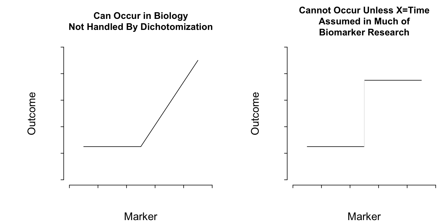
Cutpoints assume discontinuous relationships of the type in the right plot of Figure 1, and they assume that the true cutpoint is known. Beyond the molecular level, such patterns do not exist unless \(X=\)time and the discontinuity is caused by an event. Cutpoints assume homogeneity of outcome on either side of the cutpoint.
Discarding Information
Dichotomania is pervasive in biomarker research. Not only does dichotomania lose statistical information and power, but it leads to sub-optimal decision making. Consider these examples where dichotomization and incomplete conditioning leads to poor clinical thinking.
- Patient: What was my systolic BP this time?
- MD: It was \(> 120\)
- Patient: How is my diabetes doing?
- MD: Your Hb\(_{\text A1c}\) was \(> 6.5\)
- Patient: What about the prostate screen?
- MD who likes sensitivity: If you have average prostate cancer, the chance that your PSA \(> 5\) is \(0.6\)
The problem here is the use of improper conditioning (\(X > c\) instead of \(X = x\)) which loses information, and transposed conditionals, which are inconsistent with forward-in-time decision making. Sensitivity and specificity exemplify both conditioning problems. Sensitivity is \(\Pr(\text{observed~} X > c \text{~given~unobserved~} Y=y)\).
Clinicians are actually quite good at dealing with continuous markers, gray zones, and trade-offs. So why is poor conditioning so common in biomarker research done by clinical researchers?
How to Do Bad Biomarker Research
Implied Goals of Bad Research
Create a diagnostic or prognostic model that
- will be of limited clinical utility
- will not be strongly validated in the future
- has an interpretation that is not what it seems
- uses cut-points, when cut-points don’t even exist, that
- others will disagree with
- result in discontinuous predictions and thinking
- requires more biomarkers to make up for information loss due to dichotomization
- Find a biomarker to personalize treatment selection that is not as reliable as using published average treatment effects from RCTs
Study Design to Achieve Unreliable or Clinically Unusable Results
- Ignore the clinical literature when deciding upon clinical variables to collect
- Don’t allow clinical variables to have dimensionality as high as the candidate biomarkers
- Don’t randomize the order of sample processing; inform lab personnel of patient’s outcome status
- Don’t study reliability of biomarker assays or clinical variables
- Re-label demographic variables as clinical variables
- Choose a non-representative sample
- Double the needed sample size (at least) by dichotomizing the outcome measure
- Reduce the effective sample size by splitting into training and validation samples
Statistical Analysis Plan
- Don’t have one as this might limit investigator flexibility to substitute hypotheses
- Categorize continuous variables or assume they operate linearly
- Even though the patient response is a validated continuous measurement, analyze it as “high” vs. “low”
- Use univariable screening and stepwise regression
- Ignore time in time-to-event data
- Choose a discontinuous improper predictive accuracy score to gauge diagnostic or prognostic ability
- Try different cut-points on all variables in order to get a good value on the improper accuracy score
- Use Excel or a menu-based statistical package so no one can re-trace your steps in order to criticize them
Interpretation and Validation
- Pretend that the clinical variables you adjusted for were adequate and claim that the biomarkers provide new information
- Pick a “winning” biomarker even though tiny changes in the sample result in a different “winner”
- Overstate the predictive utility in general
- Validate predictions using an independent sample that is too small or that should have been incorporated into training data to achieve adequate sample size
- If the validation is poor, re-start with a different data split and proceed until validation is good
- Avoid checking the absolute accuracy of predictions; instead group predictions into quartiles and show the quartiles have different patient outcomes
- Categorize predictions to avoid making optimum Bayes decisions
What’s Gone Wrong with Omics & Biomarkers?
Subramanian and Simon (2010) wrote an excellent paper on gene expression-based prognostic signatures in lung cancer. They reviewed 16 non-small-cell lung cancer gene expression studies from 2002–2009 that studied \(\geq 50\) patients. They scored studies on appropriateness of protocol, statistical validation, and medical utility. Some of their findings are below.
- Average quality score: 3.1 of 7 points
- No study showed prediction improvement over known risk factors; many failed to validate
- Most studies did not even consider factors in guidelines
- Completeness of resection only considered in 7 studies
- Similar for tumor size
- Some studies only adjusted for age and sex
The idea of assessing prognosis post lung resection without adjusting for volume of residual tumor can only be assumed to represent fear of setting the bar too high for potential biomarkers.
Difficulties of Picking “Winners”
When there are many candidate biomarkers for prognostication, diagnosis, or finding differential treatment benefit, a great deal of research uses a problematic reductionist approach to “name names”. Some of the most problematic research involves genome-wide associate studies of millions of candidate SNPs in an attempt to find a manageable subset of SNPs for clinical use. Some of the problems routinely encountered are
- Multiple comparison problems
- Extremely low power; high false negative rate
- Potential markers may be correlated with each other
- Small changes in the data can change the winners
- Significance testing can be irrelevant; this is fundamentally a ranking and selection problem
Ranking Markers
Efron’s bootstrap can be used to fully account for the difficulty of the biomarker selection task. Selection of winners involves computing some statistic for each candidate marker, and sorting features by these strength-of-association measures. The statistic can be a crude unadjusted measure (correlation coefficient or unadjusted odds ratio, for example), or an adjusted measure. For each of a few hundred samples with replacement from the original raw dataset, one repeats the entire analysis afresh for each re-sample. All the biomarker candidates are ranked by the chosen statistic, and bootstrap percentile confidence intervals for these ranks are computed over all re-samples. 0.95 confidence limits for the rank of each candidate marker capture the stability of the ranks.
Bootstrap Ranking Example
Deming Mi, formally of the Vanderbilt University Department of Biostatistics and the Mass Spectrometry Research Lab, in collaboration with Michael Edgeworth and Richard Caprioli at Vanderbilt, did a moderately high-dimensional protein biomarker analysis. The analysis was based on tissue samples from 54 patients, 0.63 of whom died. The patients had been diagnosed with malignant glioma and received post-op chemotherapy. A Cox model was used to predict time until death, adjusted for age, tumor grade, and use of radiation. The median follow-up time was 15.5 months for survivors, and median survival time was 15 months.
213 candidate features were extracted from an average spectrum using ProTS-Marker (Biodesix Inc.). The markers were ranked for prognostic potential using the Cox partial likelihood ratio \(\chi^2\). To learn about the reliability of the ranks, 600 bootstrap re-samples were taken from the original data, and markers were re-ranked each time. The 0.025 and 0.975 quantiles of ranks were computed to derive 0.95 confidence limits. Features were sorted by observed ranks in the whole sample. The graphs below depict observed ranks, bootstrap confidence limits for them, and show statistically “significant” associations with asterisks
Results - Best

Results - Worst

One can see from the dot charts that for each candidate marker, whether it be the apparent winner, apparent weakest marker, or anywhere in between, the data are consistent with an extremely wide interval for its rank. The apparent winning protein marker (observed rank 213, meaning the highest association statistic) has a 0.95 confidence interval from 30 to 213. In other words, the data are only able to rule out the winner not being among the 29 worst performing markers out of 213. Evidence for the apparent winner being the real winner is scant.
The data are consistent with the apparent loser (rank = 1) being in the top 16 markers (confidence interval for rank [4, 198]). The fact that the confidence interval for the biggest loser does not extend to the lowest rank of 1 means that none of the 600 re-samples selected the marker as the weakest marker.
The majority of published “winners” are unlikely to validate when feature selection is purely empirical and there are many candidate features.
See this post by Peder Braadland for a beautifully annotated example.
Summary
There are many ways for biomarker research to fail. Try to avoid using any of these methods.