Assessing Heterogeneity of Treatment Effect, Estimating Patient-Specific Efficacy, and Studying Variation in Odds ratios, Risk Ratios, and Risk Differences
This article shows an example formally testing for heterogeneity of treatment effect in the GUSTO-I trial, shows how to use penalized estimation to obtain patient-specific efficacy, and studies variation across patients in three measures of treatment effect.
Vanderbilt University School of Medicine Department of Biostatistics
Published
March 25, 2019
Modified
June 7, 2024
Background
Heterogeneity of treatment effect (HTE), better called differential treatment effect, is variation in a measure of treatment effect on a scale for which it is mathematically possible that such variation be absent even if the treatment has a nonzero effect. The most commonly used scales for measuring HTE are
the original scale for continuous response variables that are properly transformed, in which case the treatment effect is the (adjusted) difference in means
odds ratios, for binary or ordinal outcomes
hazard ratios, for time-to-event outcomes
NoteSpecific Formulations of HTE
Define
\(Y\): outcome variable
\(X\): a vector of baseline patient characteristics
\(T\): treatment, with 1=new treatment and 0=standard treatment
\(F(y | X, T) = \Pr(Y \leq y | X, T)\): cumulative distribution function of \(Y\) for a given \(X\) and \(T\)
Whenever at least some of the \(X\) covariates relate to \(Y\) there will be within-treatment patient outcome variability due to these \(X\)s. When \(Y\) is a binary 0/1 response, only \(F(0 | X, T)\) is relevant and this is one minus the probability of an event (\(Y=1\)).
Let \(g\) be a one-to-one monotonic function that maps \([0, 1]\) into \([-\infty, \infty]\), i.e., \(g\) transforms the restricted \([0, 1]\) range into an unrestricted range. Some typical choices of \(g\) are as follows:
linear model: \(g(u) = \Phi^{-1}(u)\) = normal inverse transformation
binary logistic model and proportional odds ordinal logistic model: \(g(u) = \text{logit}(u) = \log\frac{u}{1-u}\) = inverse logistic transform
binary or ordinal probit model: \(g(u) = \Phi^{-1}(u)\)
\(g\) is chosen so that on the \(g(F(Y))\) scale it is possible that \(g(F(y | X, T=1)) - g(F(y | X, T=0))\) is independent of \(X\) where there is a nonzero effect of \(T\). Dependency of that difference on \(X\) means there is an \(X \times T\) interaction on the \(g\) scale. So on the \(g\) scale it is possible that no \(T\) interactions exist, i.e., interactions are surprising.
When \(g(u) = \Phi^{-1}(u)\) for continuous \(Y\) having a normal distribution with constant variance, the treatment effect is a difference in mean \(Y\): \(E(Y | X, T=1) - E(Y | X, T=0)\) which is possible to be independent of \(X\), i.e., it is possible that \(X \times T\) interactions are absent so that HTE is zero.
When \(g(u) = u\) for a binary \(Y\), we are computing differences in absolute risk. When there is any treatment effect these \(F(0 | X, T=1) - F(0 | X, T=0)\) differences must be a function of \(X\) just because of risk magnification, i.e., the differences must “slow down” as one approaches a baseline risk \(F(0 | X, T=0)\) near 0 or 1. So HTE on the untransformed probability scale will always exist and can be traced merely to generalized baseline risk. Therefore to prevent a pure statistical phenonemom from being labeled as HTE, we need to assess HTE on an unlimited \(g\) scale.
One possible way to choose \(g\) is to find the monotonic function meeting the mapping criteria that minimizes the importance of all within \(X\) and \(X \times T\) interaction effects. In a wide variety of clinical studies with binary \(Y\), the logit transformation tends to create the most additive effects and so is an excellent candidate for assessing HTE. That doesn’t mean that the logistic model will fit every situation and that odds ratios are always a magical basis for assessing HTE, but from a pragmatic standpoint the fit of logistic models is very competitive with other unrestricted range link functions \(g\).
How do we actually quantify HTE? There are two major ways:
Estimating double differences. For simplicity suppose there is only one baseline covariate, and consider two of its values: \(a, b\). Compute the differential (interaction) treatment effect \(F(y | X=a, T=1) - F(y | x=a, T=0) - [F(y | X=b, T=1) - F(y | X=b, T=0)]\).
Compute a global measure of differential treatment effect over the entire sample’s covariate distributions. Some possible measures are
deviance (-2 log-likelihood) that is due to the combined effects of all interaction effects, i.e., compute the model likelihood ratio \(\chi^2\) statistic with and without all the \(T\) interactions and take their difference
AIC, assessing whether inclusion of differential effects makes predictions of future outcomes better than ignoring them
The last idea needs to be considered more frequently, as it estimates likely out-of-sample performance of a more complex model that allows for treatment interactions. Unless the effective sample size is huge, it is often the case that pretending the HTE is absent will result in better (lower mean squared error) \(X\)-specific treatment effect estimates than allowing HTE to be present and having to estimate hard-to-estimate interaction effects. The adjusted pseudo \(R^2\) approach provides an in-sample unbiased estimate of the explanatary ability of differential treatment effects, accounting for overfitting.
Even though the more complex hazard ratio seems to be well accepted as a summary measure of treatment effect in a time-to-event randomized clinical trial (RCT), there is still a good deal of resistence to odds ratios (OR) from some clinical researchers. This resistence is difficult to understand, although it is clear that ORs are more difficult to understand than risk ratios (RR) or absolute risk reduction (ARR; risk difference). The reasons for choosing ORs are:
ORs come directly from logistic models, and logistic models are as likely as any model to fit patterns leading to binary responses. This is primarily because the logistic model places no restrictions on the regression coefficients.
ORs are capable of being constant over a range of baseline risk all the way from 0 to 1.0.
In the multitude of forest plots present in journal articles depicting RCT results, the constancy of ORs over patient types is impressive.
Unlike RRs, ORs are invariant to the choice of the “event” vs. the “no event”. If you interchange event and non-event you would get the reciprocal of the original OR, but the RR would change arbitrarily.
RR and ARR are not capable of being constant. For example, a risk factor that doubles the risk of an outcome can only apply to a patient having a baseline risk of 0.5 or less, otherwise the risk with the risk factor would exceed 1.0. A treatment that lowers the risk of an outcome of 0.04 cannot apply to a patient with a baseline risk of 0.02.
The purposes of this article are to show how
a rigorous test for HTE in the frequentist domain is done for an actual large RCT with a binary endpoint
the difficulty in estimating and testing interaction effects
the OR varies over patient types if one allows all the baseline variables to interact with treatment, whether the interactions are “significant” or not
RR varies over patient types
ARR varies over patient types
Difficulty of the Task
Establishing the existence of differential treatment effects in RCTs is difficult because RCTs are typically sized just large enough to detect an overall average treatment effect. In the ideal situation for showing evidence of HTE, a potentially interacting binary covariate yields optimum precision and power when the covariate has equal sample sizes for its two values. Even then, the precision of the interaction effect (a double difference) is four times as bad as the precision of the overall treatment effect. And as Andrew Gelman has discussed, the power is as if the sample size is divided by 16 because one typically wants to detect a differential effect that is only half as large as the overall detectable treatment effect. A related example will be shown below.
It is important to note that assessing treatment effect in an isolated subgroup defined by a categorical covariate does not establish HTE and results in unreliable estimates. Differential treatment effect must be demonstrated.
The GUSTO-I Study and Basic Outcome Model
The GUSTO-I Study was a 40,000 patient international trial comparing four treatment arms for 30-day mortality following acute myocardial infarction: streptokinase (SK) with subcutaneous heparin, SK with intravenous heparin, accelerated dosing of tissue plasminogen activator (t-PA) with intravenous heparin, and SK combined with t-PA and intravenous heparin. The covariate-adjusted analysis that forms the basis for this article was done by Steyerberg, who replaced a limited number of missing covariate values with singly imputed values. We will be primarily comparing the accelerated t-PA arm (n=10,320) with the two combined SK arms that did not involve t-PA (n=20,162).
 Value      Inferior    Other Anterior
 Frequency     23495     1435    15900
 Proportion    0.575    0.035    0.389
pmi: Previous MI
n
missing
distinct
40830
0
2
 Value         no   yes
 Frequency  34104  6726
 Proportion 0.835 0.165
tx: Tx in 3 groups
n
missing
distinct
40830
0
3
 Value      SK+tPA     SK    tPA
 Frequency   10320  20162  10348
 Proportion  0.253  0.494  0.253
Base Risk Model
A simplified covariate-adjusted risk model as developed by Steyerberg is fitted below. For simplicity when later interacting baseline variables with treatment, the important age by Killip class interaction is omitted. Pulse rate is modeled using a linear spline with a knot at 50 beats/minute.
The only way that ORs for treatment can vary in a logistic model is for there to be one or more interactions between baseline covariates and treatment. Here we allow for all interactions with treatment, which will allow ORs, RRs, and ARRs to vary as the data dictate, assuming that three-way interactions are not needed, e.g., the infarct location-specific treatment effect does not depend on age.
The likelihood ratio test is the gold-standard frequentist method for testing for added value of the treatment interactions, i.e., whether the treatment ORs are constant over covariate settings. By using a chunk test to test whether any of the baseline variables interact with treatment, this method has a perfect multiplicity adjustment in the frequentist sense.
We see no evidence to suggest HTE for t-PA or SK effects. We can also use AIC to assess whether allowing for interactions will likely result in better patient-specific outcome predictions.
Code
c(AIC(f), AIC(g))
[1] 16558.31 16581.76
The simpler model has a lower (better) AIC, indicating that treatment interactions are not strong enough to overcome the overfitting that allowing for them would entail. In other words, the interactions are likely more noise than signal.
We can also compare the two models by computing the relative explained variation on the risk scale as detailed here.
From this we see that even without penalizing for overfitting, all the treatment interactions account for only 0.004 of the predictive information. The no-interaction logit-additive model that assumes constancy of treatment ORs is at least 0.996 adequate on a scale from 0 to 1.
Back to the Difficulty of the Task
Covariate-specific treatment effects are combinations of main effects and interaction effects, and one needs evidence that the interaction effect is non-zero before covariate-specific relative efficacy is interesting. As an example of how difficult it is to estimate differential treatment effects (here, double differences on the logit scale, or ratios of odds ratios), let’s temporarily re-fit the logistic model including only a single treatment interaction—with location of infarct. Consider just inferior vs. anterior infarcts, which are the dominant categories and are not too imbalanced.
We estimate the double difference in log odds for t-PA vs. SK in anterior infarcts minus t-PA vs. SK in inferior infarcts. Then we get the frequency-weighted overall treatment effect in these two groups, which is similar to dropping the interaction from the model.
     age Killip sysbp pulse pmi  Contrast      S.E.       Lower     Upper    Z
1 61.516      I   130    73  no 0.1546134 0.1081337 -0.05732489 0.3665516 1.43
  Pr(>|z|)
1   0.1528

Confidence intervals are 0.95 individual intervals
Code
w <-with(gusto, c(sum(miloc=='Inferior'), sum(miloc=='Anterior')))contrast(i, list(tx='tPA', miloc=c('Inferior', 'Anterior')),list(tx='SK', miloc=c('Inferior', 'Anterior')),type='average', weights=w)
    Contrast       S.E.     Lower       Upper     Z Pr(>|z|)         var
1 -0.1838079 0.05588118 -0.293333 -0.07428276 -3.29    0.001 0.003122706

Confidence intervals are 0.95 individual intervals
The first contrast (double difference; differential treatment effect) has a standard error that is twice that of the second contrast (treatment effect averaged over the two infarct locations), and only the latter overall treatment effect has evidence for being non-zero (i.e., a benefit of t-PA).
Penalization
Bayesian modeling of HTE uses hierarchical random effects with shrinkage of interaction effects towards zero, e.g., shrinkage of “subgroup” effects towards the grand mean treatment effect. Borrowing information in this fashion is an optimal way to get covariate-specific treatment effect estimates. The frequentist counterpart that handles mixtures of continuous and categorical baseline variables is penalized maximum likelihood estimation. We will leave the main effects unpenalized, favoring an additive (in the log odds) model with many fewer parameters but allowing the completely unpenalized model to also have a chance at winning, and find the penalty for interaction terms that optimizes the effective AIC, i.e., the AIC computed using the effective degrees of freedom. Note that the pentrace function uses the likelihood ratio χ2 scale for AIC unlike the traditional AIC formula, i.e., here bigger AIC is better.
h <-update(g, penalty=list(simple=0, interaction=30000),maxit=30, eps=0.005)effective.df(h)
Original and Effective Degrees of Freedom

                         Original Penalized
All                            32     12.94
Simple Terms                   11     11.00
Interaction or Nonlinear       21      1.94
Nonlinear                       3      1.05
Interaction                    20      0.94
Nonlinear Interaction           2      0.05
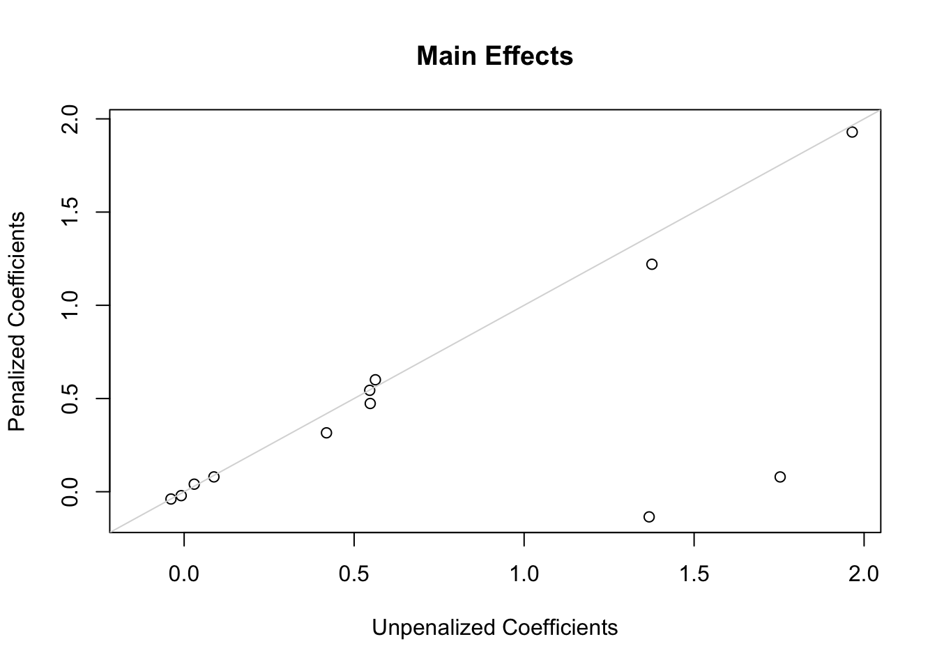
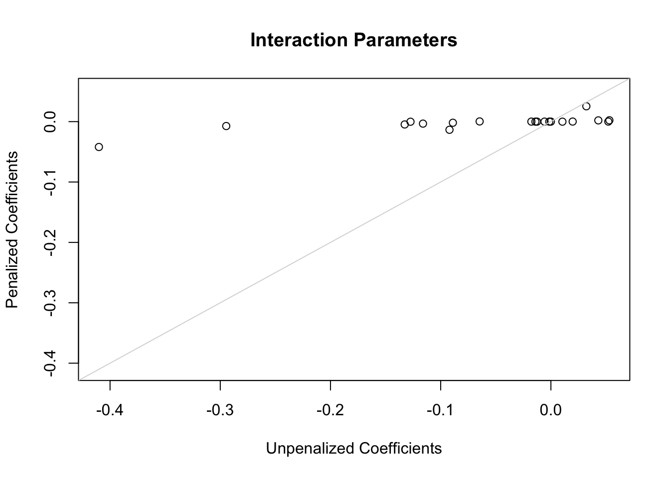
The following plots show first the main effect coefficients (with interaction effects penalized vs. not penalized), and second the interaction effect coefficients. Note that main effect coefficients can change just because of penalizing interactions, just as removing interactions from models can greatly change main effects.
Code
ia <-grep('\\*', names(coef(g)))x <-coef(g)[-c(1,ia)]; y <-coef(h)[-c(1,ia)]r <-range(c(x, y))plot(x, y,xlab='Unpenalized Coefficients',ylab='Penalized Coefficients',main='Main Effects', xlim=r, ylim=r)abline(a=0, b=1, col=gray(.85))
Code
x <-coef(g)[ia]; y <-coef(h)[ia]r <-range(c(x, y))plot(x, y,xlab='Unpenalized Coefficients',ylab='Penalized Coefficients',main='Interaction Parameters', xlim=r, ylim=r)abline(a=0, b=1, col=gray(.85))
Of the penalties studied, the best penalty by both AIC and corrected AIC is 10^{6} which effectively makes the model estimate 12.03 parameters instead of the original 12 parameters. The optimum penalty is really infinity, consistent the the likelihood ratio test for presence of any interactions with treatment. To give the benefit of the doubt we will use a penalty of 30000 to achieve an effective d.f. for interactions of 0.94.
Using the Penalized Semi-Saturated Model to Estimate Distributions of Various Effects
Even though there is no statistical evidence for HTE (i.e., interactions with treatment on an appropriate scale), we will still allow for all interactions, to give the benefit of the doubt. But we are penalizing the interaction parameters closer to what will cross-validate.
Let’s start with what I believe is the best way to communicate results to an individual patient: estimating the absolute risk of mortality under two treatment options, without hinting how the patient should summarize the two estimates (absolute vs. absolute difference, etc.). The baseline covariate values for one patient are listed below.
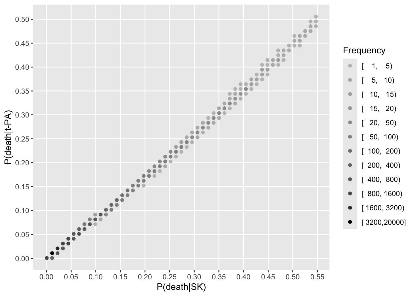
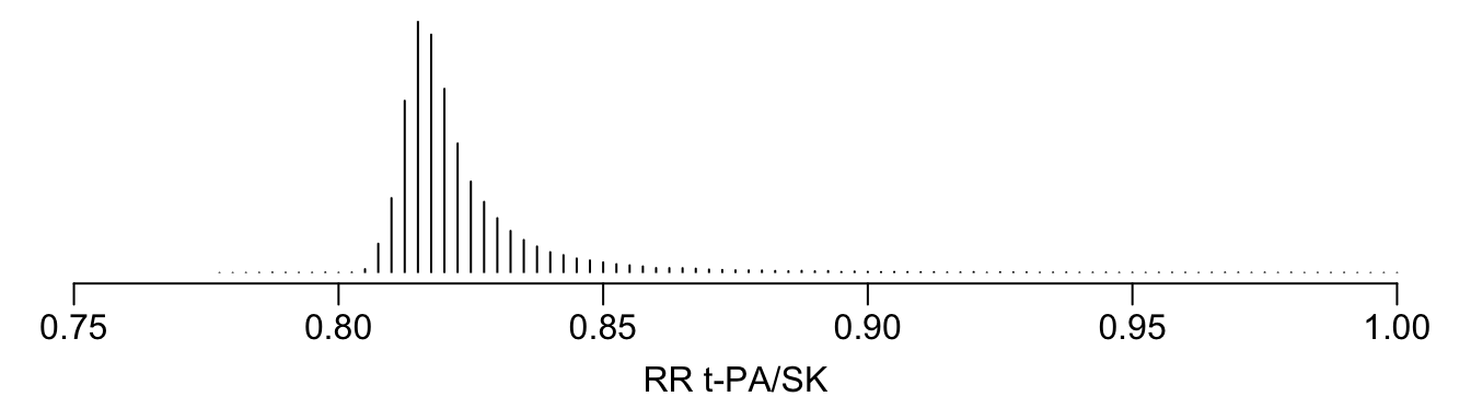
Now turn to estimating treatment effects for all the patients in the RCT. To estimate patient-specific treatment effects on various scales, we estimate risks of dying within 30 days for each patient with their own covariate settings (baseline covariate values). This is done first with treatment set to SK, no matter which treatment the patient actually received. Then predictions are done setting treatment to t-PA.
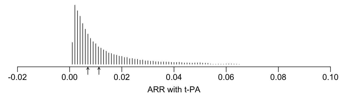
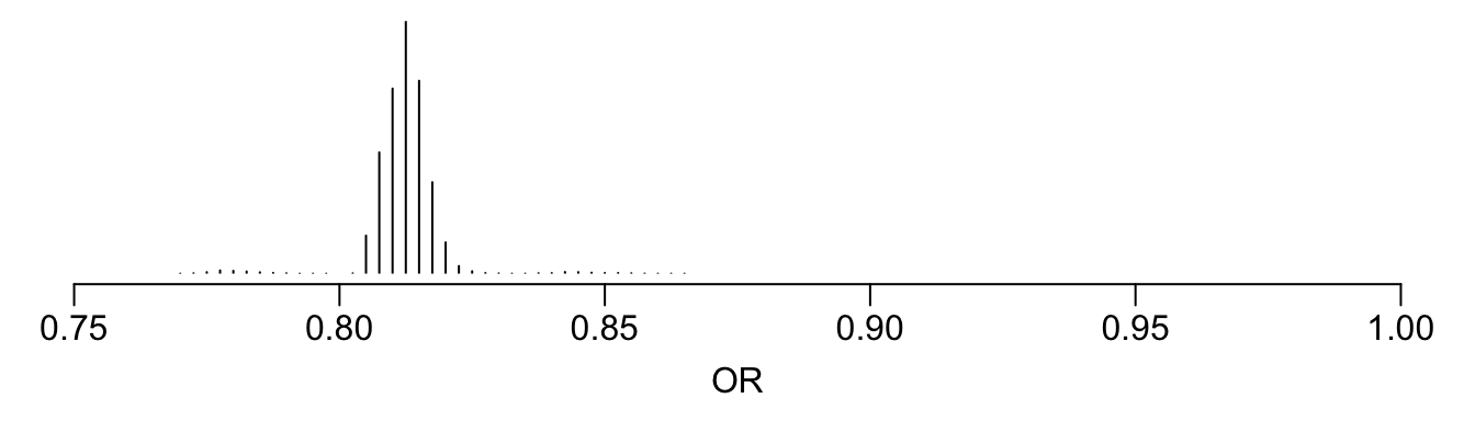
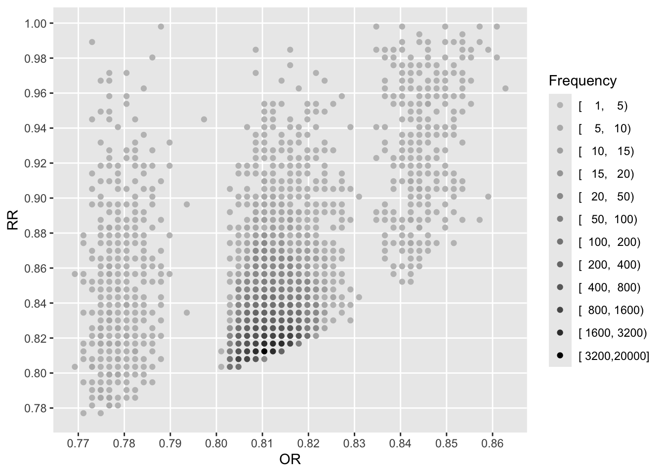
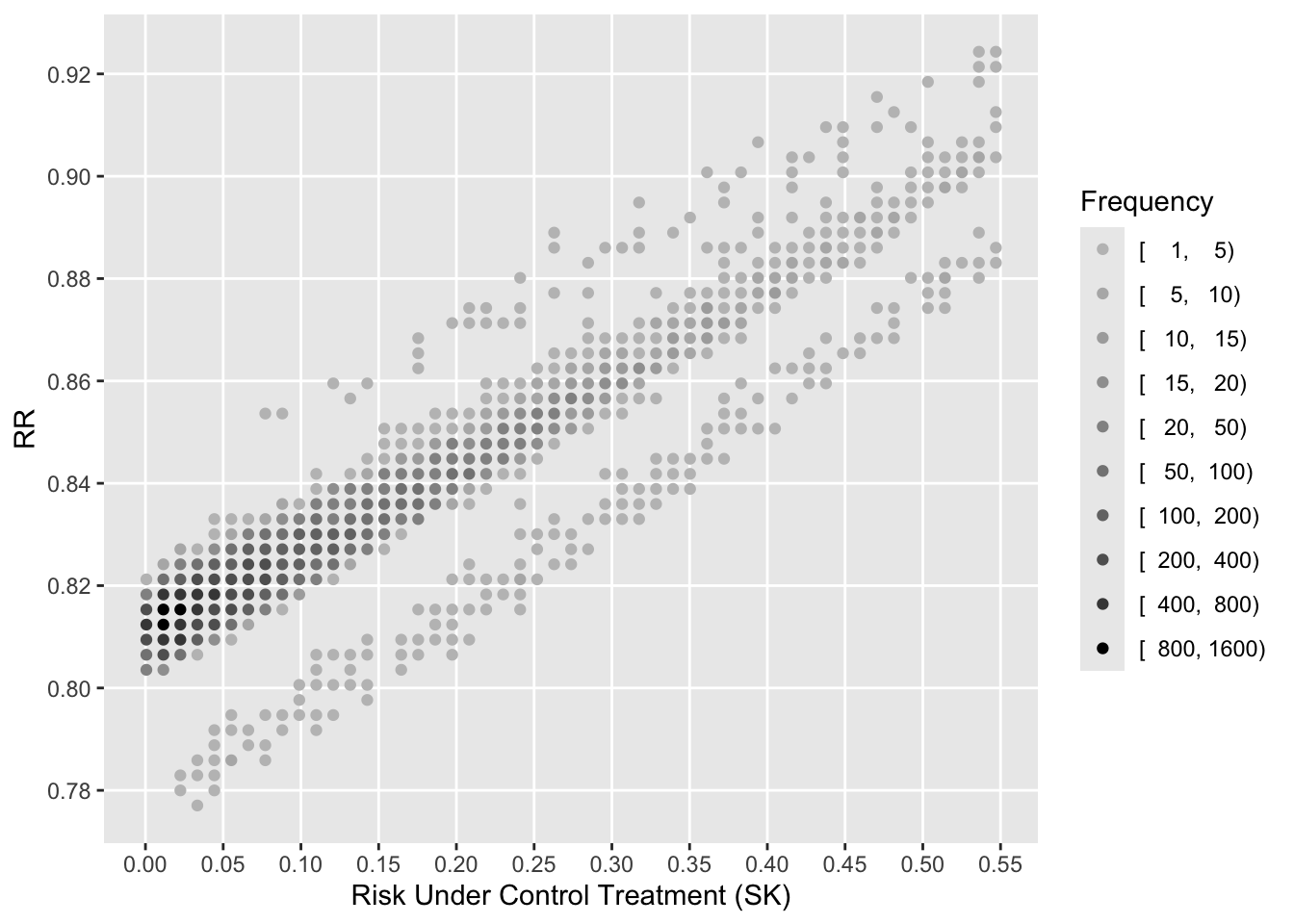
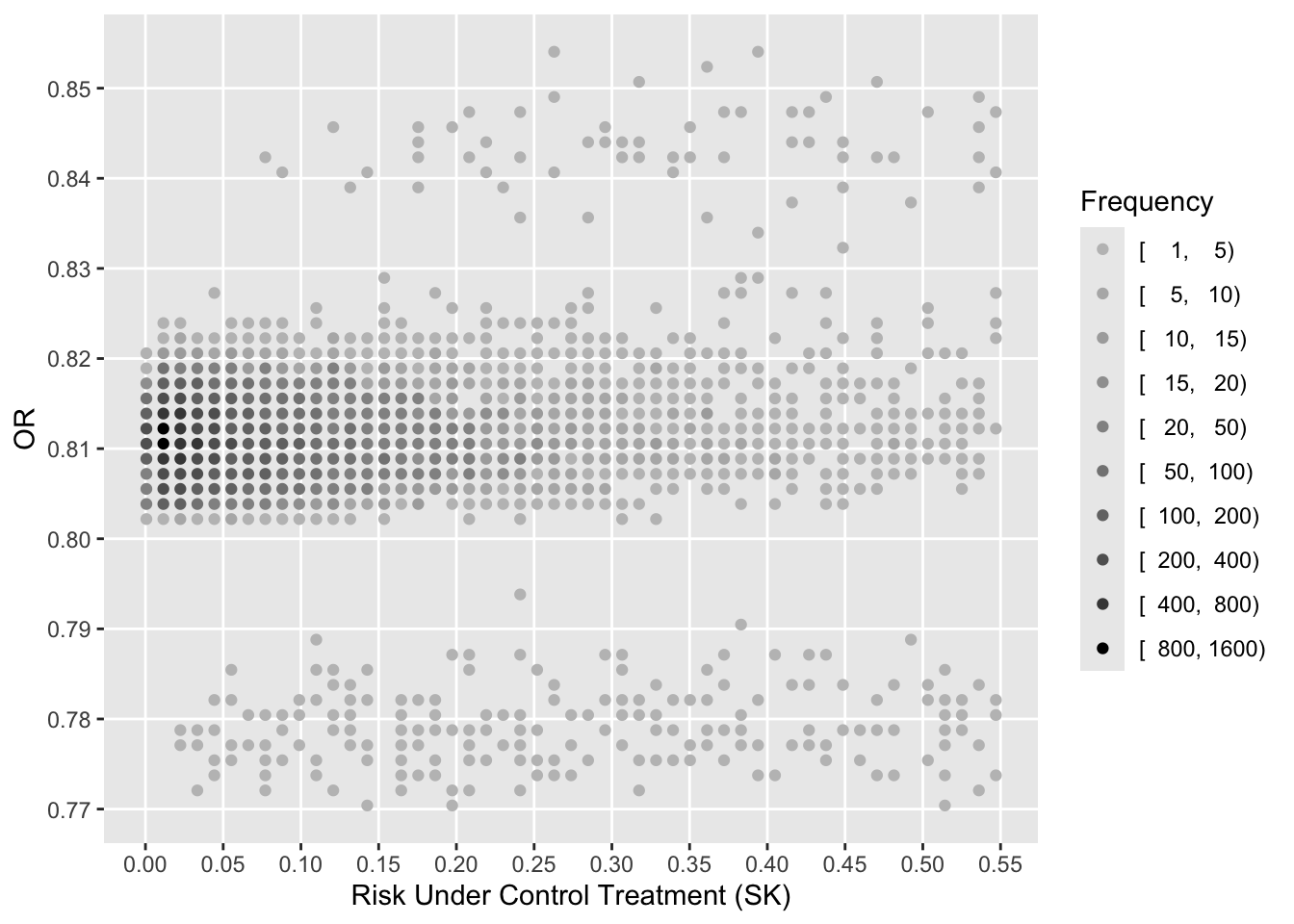
See that the variation in absolute or relative risk reduction is large, but adjusted odds ratios for t-PA vs. SK have a very narrow distribution. If we relied on the formal interaction test, this distribution would have a single value.
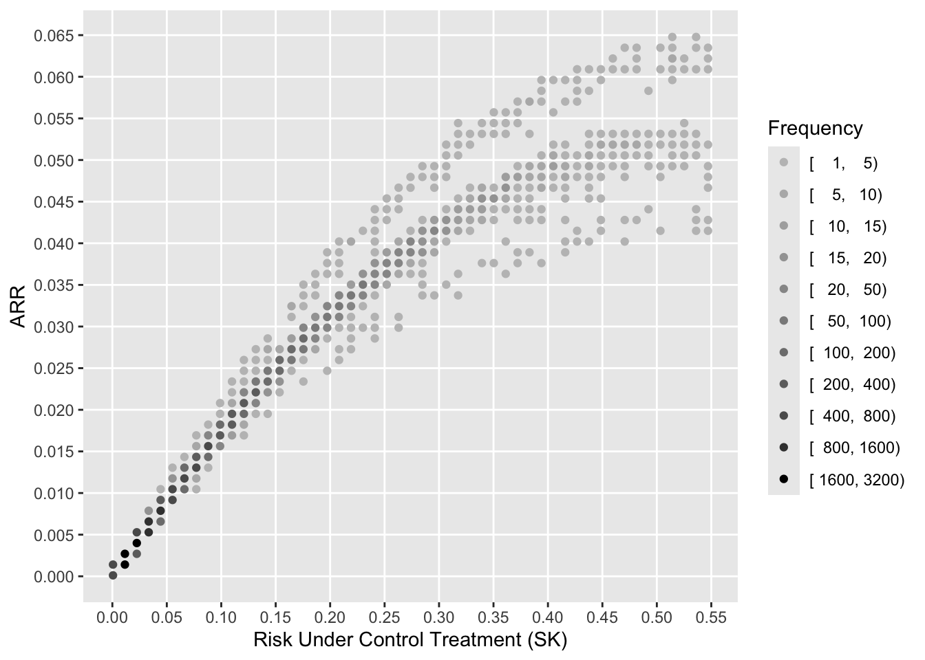
To see how the various measures depend on baseline risk, see the following graphs.
Code
xl <-'Risk Under Control Treatment (SK)'j <- psk <= plggfreqScatter(psk[j], psk[j] - ptpa[j], cuts=k, xlab=xl, ylab='ARR', fcolors=co)
---title: Assessing Heterogeneity of Treatment Effect, Estimating Patient-Specific Efficacy, and Studying Variation in Odds ratios, Risk Ratios, and Risk Differencesauthor: - name: Frank Harrell url: https://hbiostat.org affiliation: Vanderbilt University<br>School of Medicine<br>Department of Biostatisticsdate: 2019-03-25date-modified: last-modifiedcategories: [RCT, generalizability, medicine, metrics, personalized-medicine, prediction, subgroup, accuracy-score, 2019]description: 'This article shows an example formally testing for heterogeneity of treatment effect in the GUSTO-I trial, shows how to use penalized estimation to obtain patient-specific efficacy, and studies variation across patients in three measures of treatment effect.' ---## BackgroundHeterogeneity of treatment effect (HTE), better called _differential treatment effect_, is variation in a measure of treatment effect on a scale for which it is mathematically possible that such variation be absent even if the treatment has a nonzero effect. The most commonly used scales for measuring HTE are[[Discussions](http://datamethods.org/t/discussion-of-assessing-heterogeneity-of-treatment-effect-estimating-patient-specific-efficacy-and-studying-variation-in-odds-ratios-risk-ratios-and-risk-differences)<br>[Comments](https://hbiostat.org/comment.html)]{.aside}* the original scale for continuous response variables that are properly transformed, in which case the treatment effect is the (adjusted) difference in means* odds ratios, for binary or ordinal outcomes* hazard ratios, for time-to-event outcomes::: {.callout-note collapse="true"}## Specific Formulations of HTEDefine* $Y$: outcome variable* $X$: a vector of baseline patient characteristics* $T$: treatment, with 1=new treatment and 0=standard treatment* $F(y | X, T) = \Pr(Y \leq y | X, T)$: cumulative distribution function of $Y$ for a given $X$ and $T$Whenever at least some of the $X$ covariates relate to $Y$ there will be within-treatment patient outcome variability due to these $X$s. When $Y$ is a binary 0/1 response, only $F(0 | X, T)$ is relevant and this is one minus the probability of an event ($Y=1$). Let $g$ be a one-to-one monotonic function that maps $[0, 1]$ into $[-\infty, \infty]$, i.e., $g$ transforms the restricted $[0, 1]$ range into an unrestricted range. Some typical choices of $g$ are as follows:* linear model: $g(u) = \Phi^{-1}(u)$ = normal inverse transformation* binary logistic model and proportional odds ordinal logistic model: $g(u) = \text{logit}(u) = \log\frac{u}{1-u}$ = inverse logistic transform* binary or ordinal probit model: $g(u) = \Phi^{-1}(u)$* Cox proportional hazards model: $g(u) = \log(-\log(1 - u))$ (log cumulative hazard)$g$ is chosen so that on the $g(F(Y))$ scale it is possible that $g(F(y | X, T=1)) - g(F(y | X, T=0))$ is independent of $X$ where there is a nonzero effect of $T$. Dependency of that difference on $X$ means there is an $X \times T$ interaction on the $g$ scale. So on the $g$ scale it is possible that no $T$ interactions exist, i.e., interactions are surprising.When $g(u) = \Phi^{-1}(u)$ for continuous $Y$ having a normal distribution with constant variance, the treatment effect is a difference in mean $Y$: $E(Y | X, T=1) - E(Y | X, T=0)$ which is possible to be independent of $X$, i.e., it is possible that $X \times T$ interactions are absent so that HTE is zero.When $g(u) = u$ for a binary $Y$, we are computing differences in absolute risk. When there is any treatment effect these $F(0 | X, T=1) - F(0 | X, T=0)$ differences must be a function of $X$ just because of _risk magnification_, i.e., the differences must "slow down" as one approaches a baseline risk $F(0 | X, T=0)$ near 0 or 1. So HTE on the untransformed probability scale will always exist and can be traced merely to generalized baseline risk. Therefore to prevent a pure statistical phenonemom from being labeled as HTE, we need to assess HTE on an unlimited $g$ scale.One possible way to choose $g$ is to find the monotonic function meeting the mapping criteria that minimizes the importance of all within $X$ and $X \times T$ interaction effects. In a wide variety of clinical studies with binary $Y$, the logit transformation tends to create the most additive effects and so is an excellent candidate for assessing HTE. That doesn't mean that the logistic model will fit every situation and that odds ratios are always a magical basis for assessing HTE, but from a pragmatic standpoint the fit of logistic models is very competitive with other unrestricted range link functions $g$.How do we actually quantify HTE? There are two major ways:* Estimating double differences. For simplicity suppose there is only one baseline covariate, and consider two of its values: $a, b$. Compute the differential (interaction) treatment effect<br> $F(y | X=a, T=1) - F(y | x=a, T=0) - [F(y | X=b, T=1) - F(y | X=b, T=0)]$.* Compute a global measure of differential treatment effect over the entire sample's covariate distributions. Some possible measures are + deviance (-2 log-likelihood) that is due to the combined effects of all interaction effects, i.e., compute the model likelihood ratio $\chi^2$ statistic with and without all the $T$ interactions and take their difference + fraction of model $\chi^2$ due to interactions + [adjusted pseudo partial $R^2$](https://hbiostat.org/bib/r2) for the combined interaction terms + AIC, assessing whether inclusion of differential effects makes predictions of future outcomes better than ignoring themThe last idea needs to be considered more frequently, as it estimates likely out-of-sample performance of a more complex model that allows for treatment interactions. Unless the effective sample size is huge, it is often the case that pretending the HTE is absent will result in better (lower mean squared error) $X$-specific treatment effect estimates than allowing HTE to be present and having to estimate hard-to-estimate interaction effects. The adjusted pseudo $R^2$ approach provides an in-sample unbiased estimate of the explanatary ability of differential treatment effects, accounting for overfitting.:::Even though the more complex hazard ratio seems to be well accepted as a summary measure of treatment effect in a time-to-event randomized clinical trial (RCT), there is still a good deal of resistence to odds ratios (OR) from some clinical researchers. This resistence is difficult to understand, although it is clear that ORs are more difficult to understand than risk ratios (RR) or absolute risk reduction (ARR; risk difference). The reasons for choosing ORs are:* ORs come directly from logistic models, and logistic models are as likely as any model to fit patterns leading to binary responses. This is primarily because the logistic model places no restrictions on the regression coefficients.* ORs are capable of being constant over a range of baseline risk all the way from 0 to 1.0.* In the multitude of forest plots present in journal articles depicting RCT results, the constancy of ORs over patient types is impressive.* Unlike RRs, ORs are invariant to the choice of the "event" vs. the "no event". If you interchange event and non-event you would get the reciprocal of the original OR, but the RR would change arbitrarily.RR and ARR are not capable of being constant. For example, a risk factor that doubles the risk of an outcome can only apply to a patient having a baseline risk of 0.5 or less, otherwise the risk with the risk factor would exceed 1.0. A treatment that lowers the risk of an outcome of 0.04 cannot apply to a patient with a baseline risk of 0.02.The purposes of this article are to show how* a rigorous test for HTE in the frequentist domain is done for an actual large RCT with a binary endpoint* the difficulty in estimating and testing interaction effects* the OR varies over patient types if one allows all the baseline variables to interact with treatment, whether the interactions are "significant" or not* RR varies over patient types* ARR varies over patient types## Difficulty of the TaskEstablishing the existence of differential treatment effects in RCTs is difficult because RCTs are typically sized just large enough to detect an overall average treatment effect. In the ideal situation for showing evidence of HTE, a potentially interacting binary covariate yields optimum precision and power when the covariate has equal sample sizes for its two values. Even then, the precision of the interaction effect (a double difference) is four times as bad as the precision of the overall treatment effect. And as [Andrew Gelman has discussed](https://statmodeling.stat.columbia.edu/2018/03/15/need-16-times-sample-size-estimate-interaction-estimate-main-effect), the power is as if the sample size is divided by 16 because one typically wants to detect a differential effect that is only half as large as the overall detectable treatment effect. A related example will be shown below.It is important to note that assessing treatment effect in an isolated subgroup defined by a categorical covariate **does not establish HTE** and results in unreliable estimates. Differential treatment effect must be demonstrated.## The GUSTO-I Study and Basic Outcome ModelThe [GUSTO-I Study](https://www.nejm.org/doi/full/10.1056/NEJM199309023291001) was a 40,000 patient international trial comparing four treatment arms for 30-day mortality following acute myocardial infarction: streptokinase (SK) with subcutaneous heparin, SK with intravenous heparin, accelerated dosing of tissue plasminogen activator (t-PA) with intravenous heparin, and SK combined with t-PA and intravenous heparin. The covariate-adjusted analysis that forms the basis for this article was done by [Steyerberg](https://www.springer.com/us/book/9780387772431), who replaced a limited number of missing covariate values with singly imputed values. We will be primarily comparing the accelerated t-PA arm (n=10,320) with the two combined SK arms that did not involve t-PA (n=20,162).```{r setup}require(Hmisc)mu <- markupSpecs$html # in Hmiscload(url('http://hbiostat.org/data/repo/gusto.rda'))gusto <-upData(gusto, keep=Cs(day30, tx, age, Killip, sysbp, pulse, pmi, miloc))``````{r desc,results='asis'}html(describe(gusto), scroll=FALSE)```## Base Risk ModelA simplified covariate-adjusted risk model as developed by Steyerberg is fitted below. For simplicity when later interacting baseline variables with treatment, the important age by Killip class interaction is omitted. Pulse rate is modeled using a linear spline with a knot at 50 beats/minute.```{r baserisk, results='asis'}require(rms)options(prType='html')dd <-datadist(gusto); options(datadist='dd')f <-lrm(day30 ~ tx + age + Killip +pmin(sysbp, 120) +lsp(pulse, 50) + pmi + miloc, data=gusto,eps=0.005, maxit=30)f```## Semi-Saturated ModelThe only way that ORs for treatment can vary in a logistic model is for there to be one or more interactions between baseline covariates and treatment. Here we allow for all interactions with treatment, which will allow ORs, RRs, and ARRs to vary as the data dictate, assuming that three-way interactions are not needed, e.g., the infarct location-specific treatment effect does not depend on age.```{r sat, results='asis'}g <-lrm(day30 ~ tx * (age + Killip +pmin(sysbp, 120) +lsp(pulse, 50) + pmi + miloc), data=gusto,eps=0.005, maxit=60)print(g, coefs=FALSE)```The likelihood ratio test is the gold-standard frequentist method for testing for added value of the treatment interactions, i.e., whether the treatment ORs are constant over covariate settings. By using a chunk test to test whether _any_ of the baseline variables interact with treatment, this method has a perfect multiplicity adjustment in the frequentist sense.```{r lrtest}lrtest(f, g)```We see no evidence to suggest HTE for t-PA or SK effects. We can also use AIC to assess whether allowing for interactions will likely result in better patient-specific outcome predictions.```{r aic}c(AIC(f), AIC(g))```The simpler model has a lower (better) AIC, indicating that treatment interactions are not strong enough to overcome the overfitting that allowing for them would entail. In other words, the interactions are likely more noise than signal.We can also compare the two models by computing the relative explained variation on the risk scale as detailed [here](../addvalue).```{r relev}rexv <-var(predict(f, type='fitted')) /var(predict(g, type='fitted'))rexv```From this we see that even without penalizing for overfitting, all the treatment interactions account for only `r round(1 - rexv, 3)` of the predictive information. The no-interaction logit-additive model that assumes constancy of treatment ORs is at least `r round(rexv, 3)` adequate on a scale from 0 to 1.## Back to the Difficulty of the TaskCovariate-specific treatment effects are combinations of main effects and interaction effects, and one needs evidence that the interaction effect is non-zero before covariate-specific relative efficacy is interesting. As an example of how difficult it is to estimate differential treatment effects (here, double differences on the logit scale, or ratios of odds ratios), let's temporarily re-fit the logistic model including only a single treatment interaction---with location of infarct. Consider just inferior vs. anterior infarcts, which are the dominant categories and are not too imbalanced.We estimate the double difference in log odds for t-PA vs. SK in anterior infarcts minus t-PA vs. SK in inferior infarcts. Then we get the frequency-weighted overall treatment effect in these two groups, which is similar to dropping the interaction from the model.```{r ia1}i <-lrm(day30 ~ tx * miloc + age + Killip +pmin(sysbp, 120) +lsp(pulse, 50) + pmi, data=gusto,eps=0.005, maxit=30)contrast(i, list(tx='tPA', miloc='Inferior'),list(tx='SK', miloc='Inferior'),list(tx='tPA', miloc='Anterior'),list(tx='SK', miloc='Anterior'))w <-with(gusto, c(sum(miloc=='Inferior'), sum(miloc=='Anterior')))contrast(i, list(tx='tPA', miloc=c('Inferior', 'Anterior')),list(tx='SK', miloc=c('Inferior', 'Anterior')),type='average', weights=w)```The first contrast (double difference; differential treatment effect) has a standard error that is twice that of the second contrast (treatment effect averaged over the two infarct locations), and only the latter overall treatment effect has evidence for being non-zero (i.e., a benefit of t-PA).## PenalizationBayesian modeling of HTE uses hierarchical random effects with shrinkage of interaction effects towards zero, e.g., shrinkage of "subgroup" effects towards the grand mean treatment effect. Borrowing information in this fashion is an optimal way to get covariate-specific treatment effect estimates. The frequentist counterpart that handles mixtures of continuous and categorical baseline variables is penalized maximum likelihood estimation. We will leave the main effects unpenalized, favoring an additive (in the log odds) model with many fewer parameters but allowing the completely unpenalized model to also have a chance at winning, and find the penalty for interaction terms that optimizes the effective AIC, i.e., the AIC computed using the effective degrees of freedom. Note that the `pentrace` function uses the likelihood ratio `r mu$chisq()` scale for AIC unlike the traditional AIC formula, i.e., here bigger AIC is better.```{r penal}h <-update(g, x=TRUE, y=TRUE)p <-pentrace(h,list(simple=0,interaction=1000*c(1, 5, 10, 15, 20, 30, 40, 100, 200, 500, 1000)),maxit=30)ph <-update(g, penalty=list(simple=0, interaction=30000),maxit=30, eps=0.005)effective.df(h)```The following plots show first the main effect coefficients (with interaction effects penalized vs. not penalized), and second the interaction effect coefficients. Note that main effect coefficients can change just because of penalizing interactions, just as removing interactions from models can greatly change main effects.```{r showshrink}ia <-grep('\\*', names(coef(g)))x <-coef(g)[-c(1,ia)]; y <-coef(h)[-c(1,ia)]r <-range(c(x, y))plot(x, y,xlab='Unpenalized Coefficients',ylab='Penalized Coefficients',main='Main Effects', xlim=r, ylim=r)abline(a=0, b=1, col=gray(.85))x <-coef(g)[ia]; y <-coef(h)[ia]r <-range(c(x, y))plot(x, y,xlab='Unpenalized Coefficients',ylab='Penalized Coefficients',main='Interaction Parameters', xlim=r, ylim=r)abline(a=0, b=1, col=gray(.85))```Of the penalties studied, the best penalty by both AIC and corrected AIC is `r p$penalty['interaction']` which effectively makes the model estimate `r round(p$df, 2)` parameters instead of the original `r f$stats['d.f.']` parameters. The optimum penalty is really infinity, consistent the the likelihood ratio test for presence of any interactions with treatment. To give the benefit of the doubt we will use a penalty of 30000 to achieve an effective d.f. for interactions of 0.94.### Using the Penalized Semi-Saturated Model to Estimate Distributions of Various EffectsEven though there is no statistical evidence for HTE (i.e., interactions with treatment on an appropriate scale), we will still allow for all interactions, to give the benefit of the doubt. But we are penalizing the interaction parameters closer to what will cross-validate.Let's start with what I believe is the best way to communicate results to an individual patient: estimating the absolute risk of mortality under two treatment options, without hinting how the patient should summarize the two estimates (absolute vs. absolute difference, etc.). The baseline covariate values for one patient are listed below.```{r indpt}d <-data.frame(tx=c('SK', 'tPA'), Killip='II', age=55, pulse=40, sysbp=100,miloc='Inferior', pmi='no')p <-predict(h, d, type='fitted')names(p) <-c('SK', 't-PA')p```Now turn to estimating treatment effects for all the patients in the RCT. To estimate patient-specific treatment effects on various scales, we estimate risks of dying within 30 days for each patient with their own covariate settings (baseline covariate values). This is done first with treatment set to SK, no matter which treatment the patient actually received. Then predictions are done setting treatment to t-PA.```{r risks}d <- gustod$tx <-'SK'psk <-predict(h, d, type='fitted')d$tx <-'tPA'ptpa <-predict(h, d, type='fitted')k <-c(5,10,15,20,50,100,200,400,800,1600,3200,20000)pl <-c(0, quantile(psk, 0.99))j <-pmax(psk, ptpa) <= plco <-gray.colors(10, 0.75, 0)ggfreqScatter(psk[j], ptpa[j], cuts=k, fcolors=co,xlab='P(death|SK)', ylab='P(death|t-PA)')```Here is the distribution of estimated ARR across all patient types.```{r darr}#| fig-height: 2dif <- psk - ptpas <-c(mean=mean(dif), median=median(dif))shistSpike(dif, bins=seq(-0.02, 0.1, by=0.001), xlim=c(-0.02, 0.1),xlab='ARR with t-PA', minimal=TRUE)arrows(s, rep(-0.17, 2), s, rep(-.05, 2), xpd=NA, length=.05) # -0.04 -0.01 for full size```And the distribution of estimated RR.```{r drr}#| fig-height: 2histSpike(ptpa / psk, xlim=c(.75, 1), minimal=TRUE,xlab='RR t-PA/SK')```And finally the distribution of estimated ORs.```{r dor}#| fig-height: 2or <-exp(qlogis(ptpa) -qlogis(psk))histSpike(or, xlim=c(.75, 1), minimal=TRUE, xlab='OR')```The following scatterplot shows the relationship between estimated RRs and estimate ORs.```{r rror}ggfreqScatter(or, ptpa / psk, cuts=k, xlab='OR', ylab='RR', fcolors=co)```See that the variation in absolute or relative risk reduction is large, but adjusted odds ratios for t-PA vs. SK have a very narrow distribution. If we relied on the formal interaction test, this distribution would have a single value.To see how the various measures depend on baseline risk, see the following graphs.```{r vsbase}xl <-'Risk Under Control Treatment (SK)'j <- psk <= plggfreqScatter(psk[j], psk[j] - ptpa[j], cuts=k, xlab=xl, ylab='ARR', fcolors=co)ggfreqScatter(psk[j], ptpa[j] / psk[j], cuts=k, xlab=xl, ylab='RR', fcolors=co)ggfreqScatter(psk[j], or[j], cuts=k, xlab=xl, ylab='OR', fcolors=co)```## Further Reading* [Risk ratio, odds ratio, risk difference... Which causal measure is easier to generalize?](https://arxiv.org/abs/2303.16008) by Colnet, Josse, Varoquaux, Scornet* [The odds ratio is "portable" across baseline risk but not the relative risk: Time to do away with the log link in binomial regression](https://www.jclinepi.com/article/S0895-4356(21)00241-9/fulltext) by Doi, Furuya-Kanamori, Xu, Chivese, Lin, Musa, Hindy, Thalib, Harrell* [Should one derive risk difference from the odds ratio?](https://discourse.datamethods.org/t/should-one-derive-risk-difference-from-the-odds-ratio)------## DiscussionAdd your comments, suggestions, and criticisms on [datamethods.org](http://datamethods.org/t/discussion-of-assessing-heterogeneity-of-treatment-effect-estimating-patient-specific-efficacy-and-studying-variation-in-odds-ratios-risk-ratios-and-risk-differences)