```{r setup,echo=FALSE}
require(Hmisc)
getRs('reptools.r')
```
# Background
::: {.quoteit}
Data are noisy and inferences are probabilistic --- @kru15doi p. 19
:::
## Probabilistic Thinking and Decision Making
::: {.quoteit}
Optimum decisions require good data, a statistical model, and a utility/loss/cost function. The optimum decision maximizes expected utility and is a function of the Bayesian posterior distribution and the utility function. Utility functions are extremely difficult to specify in late-phase drug development. Even though we seldom provide this function we need to provide the inputs (posterior probability distribution) to decisions that will be based on an informal utility function.
:::
* Statistics: judgment and decision making under uncertainty
* Decision maker must understand key uncertainties
* To understand uncertainty one must understand probability
* Know the conditions being assumed and the event or assertion we are estimating the prob. of
* Most useful probs: Prob(something unknown) conditioning on or assuming something *known*
* Forward time/information flow
[Interactive demo of conditional probability](http://setosa.io/conditional)
Compare backwards and forwards probs<br>
PP = Bayesian posterior ("post data") probability
Type | Backwards Probability | Forwards Probability
---- | --------------------- | --------------------
Forecast | P(current state \| future event occurs) | P(future event \| current state)
Diagnosis | P(positive test \| disease) (sensitivity) | P(disease \| positive test)
Disease Incidence | P(black \| has diabetes) | P(diabetes \| black)
General | P(data \| assertion X) | P(assertion X true \| data)
P-value vs. PP | P(data **in general** more extreme \| no effect) | P(effect \| **these** data)
Aside:
* Optimum medical dx and treatment = maximizing expected utility (@vic08dec)
* Expected utility is a function of forward Prob(disease) and not sens and spec
Order of conditioning all-important
Probability Statement | Meaning | Value
----------- | ------------ | -------
P(female \| senator) | of senators what prop. are female | 21/100
P(senator \| female) | of females what prop. are senators | 21/165M
Translation of assertions into probability statements:
Assertion | Probability Statement
--------- | ---------------------
50 year old has disease now | P(disease \| age=50)
disease-free 50 y.o. will get a disease within 5y | P(T ≤ 5 \| age=50)<br>T = time until disease
50 y.o. male has disease | P(disease \| age=50 and male)
A drug really lowers blood pressure | P(θ < 0 \| data)<br>θ=unknown bp Δ, data=RCT data
Drug ↓ blood pressure or ↑ exercise time | P(θ<sub>1</sub> < 0 or θ<sub>2</sub> > 0 \| data)<br>θ<sub>1</sub>=unknown bp Δ, θ<sub>2</sub>=unknown ex. time Δ
@spi86 classic paper: power of forward probs. in decision making about patient management \& clinical trials
Advantages when prob is P(assertion of direct interest):
* Forward prob self-contained and defines its own error probability for decision making
* P(efficacy) = 0.96 ⇒ P(error) = P(drug ineffective or harmful) = 0.04
* vs. 1 - type I error = P(others will get data less extreme than ours if exactly zero effect of drug)
::: {.quoteit}
Thus to claim that the null P value is the probability that chance alone produced the observed association is completely backwards: The P value is a probability computed assuming chance was operating alone. The absurdity of the common backwards interpretation might be appreciated by pondering how the P value, which is a probability deduced from a set of assumptions (the statistical model), can possibly refer to the probability of those assumptions. --- @gre16sta
:::
## Bayes' Theorem
* Basis for Bayesian estimation and inference
* Is a condition-reversal formula
* Consider condition $A$ vs. not $A$ (denoted $\overline{A}$)
* Consider condition $B$ vs. not $B$ (denoted $\overline{B}$)
* The theorem comes from laws of conditional and total probability
* $P(A|B)$ = prob that condition $A$ holds given that condition $B$ holds, and similarly for $P(B|A)$
* $P(A)$ is prob that $A$ holds regardless of $B$, and likewise for $P(B)$
Bayes' theorem is stated as
$$P(B|A) = \frac{P(A|B) \times P(B)}{P(A)}$$
To avoid dealing with the marginal probability of $A$, Bayes re-expressed the last equation.
Consider the case where $B$ can take on only two values $B$ and $\overline{B}$: $$P(B|A) = \frac{P(A|B) \times P(B)}{(1-P(B)) \times P(A|\overline{B}) + P(B) \times P(A|B)}$$
This can be written as posterior odds = prior odds $\times$ likelihood ratio since a probability equals $\frac{\text{odds}}{1 + \text{odds}} = \frac{1}{\frac{1}{\text{odds}} + 1}$:
$$
\frac{P(B|A)}{1 - P(B|A)} = \frac{P(B)}{1 - P(B)} \times \frac{P(A|B)}{P(A|\overline{B})}
$$
Bayes' rule is visualized in the 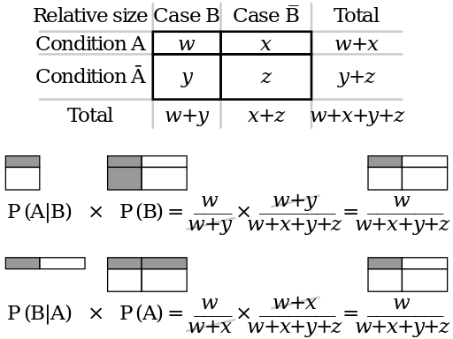
Contingency table illustrating Bayes' theorem, from [Wikimedia Commons](https://commons.wikimedia.org/wiki/File:Bayes_theorem_visualisation.svg). $w$ $x$ $y$ and $z$ represent frequency counts. Think of Condition $A$ as representing a positive diagnostic test, condition not $A$ (Condition $\overline{A}$) as a negative test, Case $B$ as "diseased" and Case $\overline{B}$ as "non-diseased".
* Will use Bayes' theorem to make a prob statement about drug effect given data
* Data model is a function of the unknown drug effect
* [Video tutorial](https://youtu.be/5NMxiOGL39M) on Bayes basics
* [Introduction to Bayesian Statistics by Woody Lewenstein](https://youtu.be/NIqeFYUhSzU?si=fECV43EcRCMM6KXI) video
::: {.quoteit}
Bayes' theorem dictates that two individuals starting with the same beliefs (distribution) about an unknown parameter, who are given the same data, use the same data model, and agree not to redefine their prior beliefs after seeing the data, must have identical beliefs about the parameter (same conclusion about drug effectiveness) after analyzing the data.
:::
## What is a Posterior Probability?
* Bayes incorporates baseline beliefs (prior) with observed data (trial results) to get posterior prob (PP)
* Flexibility to ask multiple and complex questions
+ What is P(drug has at least a specific effect size **and** avoids a specific adverse effect)
* Posterior density function: like a histogram
+ x-axis: drug effect size
+ y-axis: prob or relative degree of belief in that effect size
* Uses:
+ area under curve from a to b is P(effect between a and b)
+ area to the right of b is P(effect > b)
* Answers the question clinicians and regulators most interested in:
+ What is P(drug does X) <br>**not**<br>
+ P(observing an even larger observed effect if the drug does nothing)
* Frequentist probs:
+ long-run relative frequencies
+ don't apply to one-time events, e.g. experiments that cannot be repeated
* Bayesian PPs:
+ can be fully objective/mechanistic/long-run rel. freq. as in upcoming coin flipping example
+ usually we don't have unassailable truth for prior knowledge, so anchor is quantified by a degree of belief
+ But if we have a certain pre-data belief, Bayes' theorem dictates the post-data degree of belief we **must** have
+ uses new evidence to update a prior prob to a PP
+ the entire Bayesian machine can be derived from the most basic axioms of probability (e.g., the sum of all probs over all possibilities is 1.0)
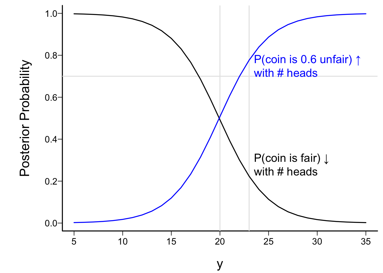
## Example: Prior to Posterior
* Novelty coin maker makes biased coin with P(heads)=0.6
* He randomly mixes in fair coins; 3/10 of coins are fair
* Choose a coin from the whole batch at random, toss 40 times
* Observe 23 heads out of 40 tosses
* Let θ=unknown probability of heads
* Only 2 values of θ are possible: 0.5 and 0.6
* Prior distribution for θ has two values where probability is nonzero
* Prior distribution is zero for θ ≠ 0.5 or 0.6
* Let y = observed number of heads
* PP(θ = 0.5) proportional to $0.3 \times 0.5 ^ {y} \times 0.5 ^ {n - y}$
* PP(θ = 0.6) proportional to $0.7 \times 0.6 ^ {y} \times 0.4 ^ {n - y}$
* Summing these two provides the normalizing constant to make them sum to 1.0
* Shown as a function of y in figure below, for n=40
```{r discrete}
#| fig.cap: "Posterior P(θ=0.5|y) (black curve) and P(θ=0.6|y) (blue curve) as a function of the observed number of heads y after 40 coin tosses. The prior probability that θ=0.6 is shown with a horizontal grayscale line. Vertical grayscale lines are shown at y=20 and at the observed number of heads, y=23. Prior probabilities that θ=0.5, 0.6 are 0.3 and 0.7."
#| fig.scap: "Posterior probabilities after coin tosses"
spar(bty='l')
prior1 <- 0.3; prior2 <- 0.7
n <- 40
y <- 5:35
post1 <- prior1 * (0.5 ^ y) * (0.5 ^ (n - y))
post2 <- prior2 * (0.6 ^ y) * (0.4 ^ (n - y))
total <- post1 + post2
post1 <- post1 / total
post2 <- post2 / total
plot(y,  post1, type='n',
     xlab=expression(y), ylab='Posterior Probability')
abline(v=c(20, 23), col=gray(.9))
abline(h=prior2, col=gray(.9))
lines(y, post1)
lines(y, post2, col='blue')
text(23.5, 0.75, 'P(coin is 0.6 unfair) ↑\nwith # heads',
     col='blue', adj=0)
text(23.5, 0.28, 'P(coin is fair) ↓\nwith # heads', adj=0)
op1 <- round(post1[y == 23], 2)
op2 <- round(post2[y == 23], 2)
```
* With y=23, PPs are 0.22 and 0.78 so evidence for fairness has lessened over what we had in the prior
* Breakeven point y=20: equally likely to be fair or biased (because predisposition to be biased)
## Bayesian Inference Model: General Case
* Above example had only limit number of possibilities for θ
* Usually have a continuous *parameter space* for θ (difference in means, etc.)
* Must use *prob density functions* instead of discrete probs
* pdf: P(θ in a small interval) divided by width of interval as width → 0
* General Bayes formula: p(θ | data y) ∝ p(y | θ) p(θ) = data likelihood × prior<br>prior belief about θ $\stackrel{\text{data}}{\longrightarrow}$ current belief about θ
* See [Wasserman](http://www.stat.cmu.edu/~larry/=stat705/lecture14.pdf) for a nice overview of the general Bayes equation
* **If** you have degree of belief p(θ) before seeing data from the experiment you **must** have degree of belief p(θ|y) after unveiling the data
* Summarize posterior density p(θ|y) by posterior means, quantiles, cumulative probs, interval probs
* Must integrate out θ to get such quantities
* Easier to sample from posterior than to derive posterior mathematically
### Example
#### @lap17eff: Bayesian RCT of hypothermia > 6h of birth with ischemic encephalopathy {-}
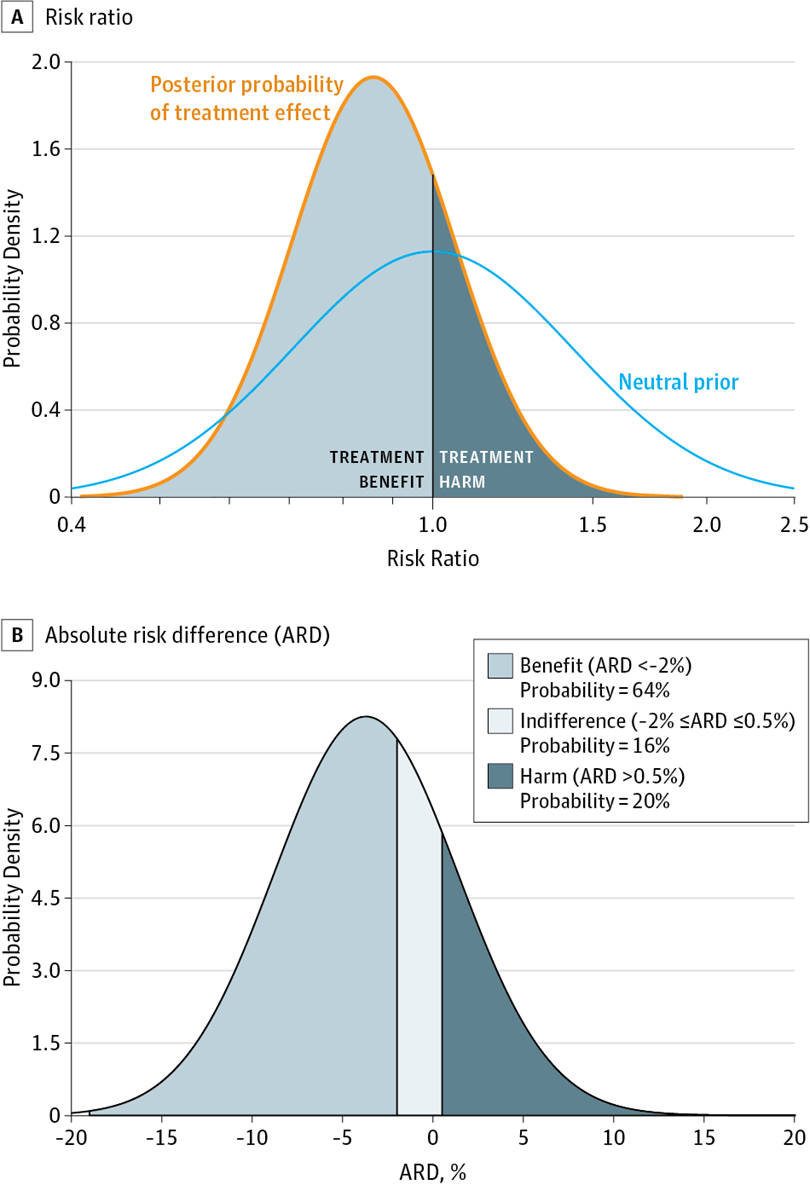{width=600px}<br>{width=600px}
### One-Sample Mean Examples
The following examples are for the simple case where the data come from a normal distribution with standard deviation 1.0, and we are interested in estimating the unknown mean μ which is responsible for generating the data. Large values of μ are "better", and we assume a prior distribution for μ which is normal with mean zero, and with various values of σ. In this "normal data, normal prior" case, the posterior distribution is also a normal distribution. The variance of the posterior distribution is the geometric mean of the prior variance and the variance of $\overline{x}$. The mean of the posterior is a weighted average of the prior mean and $\overline{x}$, with weights equal to, respectively, the ratio of the posterior variance to the prior variance, and the ratio of the posterior variance to the variance of $\overline{x}$ (which in our situation is 1/n). When the prior mean is zero, the posterior mean is just a shrunken version of $\overline{x}$.
In specifying a prior distribution it is often convenient to specify an effect size and a probability that the size exceeds that.
The prior SD σ is computed here so that the prior probability P(μ > 2) matches a specified value (either 0.01, 0.05, or 0.25). Larger chances of μ being large correspond to larger σ. The observed sample mean $\overline{x} is set at three possible values: 0, 1, 2.
::: {.panel-tabset}
#### n=5 {-}
```{r preposts}
require(plotly)
ppost <- function(n) {
  d <- expand.grid(xbar=0:2, Plarge=c(.01, .05, .25))
  p <- plot_ly()
  for(i in 1 : nrow(d)) {
    w      <- d[i, ]
    xbar   <- w$xbar
    plarge <- w$Plarge
    psigma <- 2 / qnorm(1 - plarge)
    vs     <- 1 / sqrt(n)
    vpre   <- psigma ^ 2
    vpost  <- 1 / (1 / vpre + 1 / vs)
    mpost  <- xbar * vpost / vs
    mu     <- seq(-3, 3, by=0.02)
    lab    <- paste0('<span style="text-decoration: overline">x</span>=', xbar, ' prior P(μ > 2)=', plarge)
    pp     <- dnorm(mu, mpost, sqrt(vpost))
    priorp <- dnorm(mu, 0, psigma)
    vis <- if(i == 1) TRUE else 'legendonly'
    p <- p %>% add_lines(x=~mu, y=~priorp, hoverinfo='none', visible=vis, legendgroup=lab,
                         name=paste0(lab, ':', 'prior'), opacity=0.2, data=data.frame(mu, priorp))
    pexceed <- 1 - pnorm(mu, mpost, sqrt(vpost))
    txt <- paste0('μ=', round(mu, 2), ' P(μ > ' , round(mu, 2), ')=', round(pexceed, 2))
    p <- p %>% add_lines(x=~mu, y=~pp, text=~txt, hoverinfo='text',
                         visible=vis, legendgroup=lab,
                         name=paste0(lab, ':', 'posterior'), data=data.frame(mu, pp, txt))
  }
  p %>% layout(xaxis=list(title='μ'),
               yaxis=list(title='Probability Density Function', range=c(0, 1.35)))
}
ppost(5)
```
#### n=10 {-}
```{r}
ppost(10)
```
#### n=25 {-}
```{r pp3}
ppost(25)
```
#### n=100 {-}
```{r pp4}
ppost(100)
```
:::
### Links to More Examples
* Interactive [visualization](http://rpsychologist.com/d3/bayes) of a 2-sample t-test
* Interactive Bayesian inference for [2-arm RCT](http://medstats.atspace.cc/bayes.html) with binary endpoint
* More [examples](https://stats.stackexchange.com/questions/58564/help-me-understand-bayesian-prior-and-posterior-distributions) of prior, likelihood, and posterior
* John Kruschke's [Bayesian t-test](http://www.indiana.edu/~kruschke/BEST) web page
* John Kruschke's [blog](http://doingbayesiandataanalysis.blogspot.com)
* Online resource for [Bayesian decision making](http://www.statsathome.com/2017/10/12/bayesian-decision-theory-made-ridiculously-simple)
## What is Bayesian Inference Doing?
::: {.panel-tabset .quoteit}
### Quotes
### FH
Bayesian data analysis is a clear conceptual framework for learning
### Edwards, Lindman, Savage
The Bayesian approach is a common sense approach. It is simply a set of techniques for orderly expression and revision of your opinions with due regard for internal consistency among their various aspects and for the data --- @edw63bay
### FH
Type I error for smoke detector: probability of alarm given no fire<br><br>
Bayesian posterior probability: probability there's a fire given current air data, whether or not an alarm is triggered
<br><br>
Smoke detector designed by a frequentist investigator who runs single-site RCTs: require a 0.05 false alarm probability, and require a probability (power) of 0.8 to detect an inferno
<br><br>
Actionable probabilities with a Bayesian smoke detector: set to sound an alarm if the probability of a fire exceeds 0.02 while you are at home or exceeds 0.01 while you are away
:::
* Bayes approach to inference & decision making: condition on what is known to make prob statements about what isn't
* Frequentist has to use "proof by contradiction" and reason using reverse time/information flow
* Creates difficulties with
+ multiplicities
+ adaptive designs
+ confusion in how null hypothesis is conceived (e.g., non-inferiority study)
+ no unique prescription for deriving multiplicity adjustments
+ no way to incorporate extra-study info
+ no evidential statements re:totality of evidence
* Contrast with Bayesian statement:
+ prob that drug does not raise mortality by more than 0.04 and either
- lowers mortality by any amount<br>or
- improves exercise time by > 5m<br>or
- lowers bp by > 2 mmHg
::: {.panel-tabset .quoteit}
### Quotes
### Gelman
Frequentist inference has the virtue and drawback of being multi-focal of having no single overarching principle of inference. From the user's point of view, having multiple principles (unbiasedness, asymptotic efficiency, coverage, etc.) gives more flexibility and, in some settings, more robustness with the downside being that application of the frequentist approach requires the user to choose a method as well as a model. --- @gel15bay
### Gelman
[Bayesian methods are often characterized](http://rwconnect.esomar.org/the-abcs-of-bayesian-basics) as 'subjective' because the user must choose a 'prior distribution', that is, a mathematical expression of prior information. The prior distribution requires information and user input, that's for sure, but I don't see this as being any more 'subjective' than other aspects of a statistical procedure, such as the choice of model for the data (for example, logistic regression) or the choice of which variables to include in a prediction, the choice of which coefficients should vary over time or across situations, the choice of statistical test, and so forth. Indeed, Bayesian methods can in many ways be more `objective' than conventional approaches in that Bayesian inference, with its smoothing and partial pooling, is well adapted to including diverse sources of information.
:::
### Simulations Expose Logic Flow
* Simulations are useful for understanding the logic of inferential methods
* Real simulation examples shown later
* Estimation example: one-sample problem to estimate population mean μ
+ frequentist
- choose a single value of μ
- generate data from a population with mean μ
- see how close the point estimate is to μ
+ Bayesian
- choose a prior distribution for μ
- from that distribution sample 1000 values of μ
- for each μ generate data from a population with mean μ
- make a scatterplot of true μ vs. posterior mean, median, or mode
- use a nonparametric smoother to estimate the calibration curve (x=point estimate, y=μ)
- note that Bayesian don't always like to make point estimates, leaving the posterior density as the final result
## The Use of Prior Information ... Or Not
* Bayesian methods condition on what is "known" so important to define "known" aside from the observed data. Examples of what is known:
+ nothing (use of a flat or non-informative prior distribution)
+ evidence from other studies of the same drug or device
+ evidence from other studies of the same class of drug or device
+ evidence from a previous clinical trial for which the current trial is a replication
+ evidence about the same treatment in a different patient population
+ historical evidence from observational studies
+ skepticism that a treatment can have major efficacy because either
- multiple previous clinical trials in the drug class were "negative""
- the reviewer who needs to be convinced of an effect is a skeptic
* Bayes may require fewer or more subjects
* Bayes does **not** require one to use prior data or expert opinion
- can use data with any prior: non-informative, skeptical, optimistic
* Reviewers have say in
+ prior
+ adequate level of PP is convincing
+ which effect cutoff to compute PP for
* Problems with just using default non-informative (flat) priors
+ allows for arbitrarily large treatment benefit or harm
+ no constraints to what is mathematically, pharmacologically, or clinically possible
+ increases P(benefit when treatment actually harms)
+ if study is stopped early, easy to overstate efficacy
* It is not possible to preserve type I error when incorporating external information into an analysis (@kop19pow)
* [Guidance](https://github.com/stan-dev/stan/wiki/Prior-Choice-Recommendations) for selection of priors (statistical issues)
::: {.panel-tabset .quoteit}
### Quotes
### Kruschke
Prior beliefs are overt, explicitly debated, and founded on publicly accessible previous research. A Bayesian analyst might have personal priors that differ from what most people think, but if the analysis is supposed to convince an audience, then the analysis must use priors that the audience finds palatable. It is the job of the Bayesian analyst to make cogent arguments for the particular prior that is used. The research will not get published if the reviewers and editors think that the prior is untenable. Perhaps the researcher and the reviewers will have to disagree about the prior, but even in that case the prior is an explicit part of the argument, and the analysis should be conducted with both priors to assess the robustness of the posterior. Science is a cumulative process, and new research is presented always in the context of previous research. A Bayesian analysis can incorporate this obvious fact. ... the priors are overt, public, cumulative, and overwhelmed as the amount of data increases. Bayesian analysis provides an intellectually coherent method for determining the degree to which beliefs should change. --- @kru15doi p. 317
### FH
Any frequentist criticizing the Bayesian paradigm for
requiring one to choose a prior distribution must recognize that she
has a possibly more daunting task: to completely specify the
experimental design, sampling scheme, and data generating process
that were actually used and would be infinitely replicated to allow
p-values and confidence limits to be computed.
### Krushke & Liddell
In the early years, many people had philosophical concerns about the status of the prior distribution, thinking that the prior was too nebulous and capricious for serious consideration. But many years of actual use and real-world application have allowed reality to overcome philosophical anxiety.<br><br>
... the practical results along with the rational coherence of the approach have trumped earlier concerns. The remaining resistance stems from having to displace deeply entrenched and institutionalized practices. --- @kru17bay
### Gelman
The default conclusion from a noninformative prior analysis will almost invariably put too much probability on extreme values. A vague prior distribution assigns much of its probability on values that are never going to be plausible, and this disturbs the posterior probabilities more than we tend to expect---something that we probably do not think about enough in our routine applications of standard statistical methods. -- @gel13pva
### McElreath
If your goal is to lie with statistics, you'd be a fool to do it with priors, because such a lie would be easily uncovered. Better to use the more opaque machinery of the likelihood. Or better yet---don't actually take this advice!---massage the data, drop some "outliers", and otherwise engage in motivated data transformation. --- @mce16sta
:::
### Priors That Merely Exclude Impossible Values
* Examples:
+ SD > mean for positive-valued Y
+ Tx effect > anything ever observed for disease or drug class
* Sometimes take prior prob distribution as flat within the interval of possibility
* If observed data more extreme than this, posterior distribution will have "wall" at the constraint<br>Posterior mode/mean/median will still be impressive
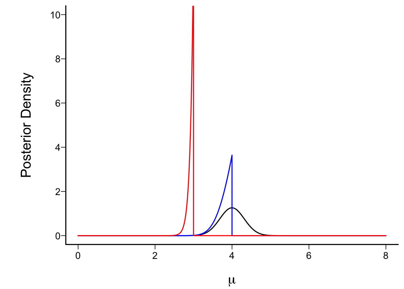
* Consider 1-sample problem: estimate μ when σ=1
* Use range of plausibility for μ as [a, b]<br>Prior flat inside [a,b], 0 outside
* Take observed sample mean to be 4 with n=10
```{r trunc}
#| fig.cap: "Posterior density functions under flat priors over different intervals. Black: interval of possibility for μ is [0,6]; Blue: interval is [0,4]; Red: interval is [0,3]. The black posterior density function is the limit of heights of the bars in the next figure divided by the bar width, as the width approaches zero."
spar(bty='l')
# Function to compute the posterior density with a truncated flat prior over x in [a,b]
# x=observed sample mean, s=population SD, n=sample size
pp <- function(x, a, b, s=1, n, xlim=c(0, 8)) {
    s <- s / sqrt(n)
    mu <- if(missing(a)) seq(xlim[1], xlim[2], length=150)
    else
      seq(a, b, length=150)
    eps <- 0.00001
    mus <- seq(min(mu), max(mu), by=eps)

    if(missing(a)) return(list(x=mu, y=dnorm(mu, mean=x, sd=s)))
    # http://math.stackexchange.com/questions/1787177
    y <- dnorm(x, mu, s) / (pnorm(b, mu, s) - pnorm(a, mu, s)) *
         (mu >= a & mu <= b)
    # Evaluate on a finer grid for numerical integration
    yf <- dnorm(x, mus, s) / (pnorm(b, mus, s) - pnorm(a, mus, s)) *
         (mus >= a & mus <= b)
    # Get area under the density function because we may only have the function
    # up to a constant of proportionality
    area <- eps * sum(yf[-1] + yf[-length(yf)]) / 2  # trapezoid rule
    y <- y / area; yf <- yf / area
    # Also compute posterior cumulative distribution function at selected mu's
    mus2 <- seq(2.5, 5.5, by=0.25)
    cdf <- approx(mus, eps * cumsum(yf), xout=mus2)
    list(x=c(xlim[1], a, mu, b, xlim[2]), y=c(0, 0, y, 0, 0), cdf=cdf)
}
plot(pp(x=4, n=10, a=0, b=6), type='l', ylim=c(0,10),
     xlab=expression(mu), ylab='Posterior Density')
lines(pp(x=4, n=10, a=0, b=4), col='blue')
lines(pp(x=4, n=10, a=0, b=3), col='red')
```
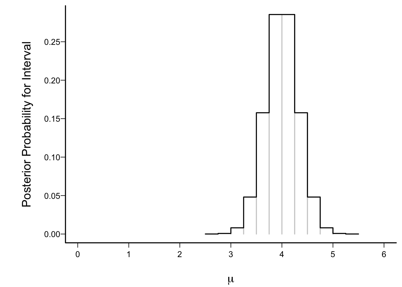
* To better understand posterior density functions (relative degree of belief after seeing the data), make histogram-like plot
* Intervals of width 0.25 for the flat prior on [0,6]
* Height of a bar = P(μ is in that interval)
```{r trunchist}
#| fig.cap: "Posterior interval probabilities under a flat prior over the interval μ ∈ [0,6]"
#| fig.scap: "Posterior interval probabilities"
spar(bty='l', ps=13)
cdf <- pp(x=4, n=10, a=0, b=6)$cdf
xs  <- cdf$x
interval.probs <- diff(cdf$y)
plot(0, 0, xlim=c(0,6), ylim=c(0, max(interval.probs)), type='n',
     xlab=expression(mu), ylab='Posterior Probability for Interval')
segments(xs[-1], 0, xs[-1], interval.probs, col=gray(.8))
lines(c(xs[1], rep(xs[-1], each=2)),
      c(rep(interval.probs, each=2), interval.probs[length(interval.probs)]))
```
## Bayesian Inferences are Exact, To Within Simulation Error
* P-values are often less accurate than we care to admit
* Only a handful of settings have exactly correct p-values
+ linear model with normal residuals and constant variance
+ its special case the 2-sample t-test with equal var.
+ one-sample t-test with normality
+ certain tests from exponential distributions
+ Wilcoxon and Wilcoxon signed-rank tests with no ties
* Methods assuming large-sample normality often require much larger n than assumed
* Models with very non-quadratic log-likelihood functions esp. problematic
+ e.g. binary logistic model
* With sequential tests we seldom know how to compute p
* Bayesian approach: exact, if data model correctly specified
* If can't derive the posterior distribution, use simulation methods
+ these give exact probs to within simulation error
+ run tens of thousands of draws from posterior


