9 Bayesian Clinical Trial Design
Example
A prototype Bayesian sequential design meeting multiple simultaneous goals will be discussed. The design includes selection of outcome variables and specification of honest effect sizes for computing Bayesian power and doesn’t take sample size calculations too seriously. The design has excellent Bayesian operating characteristics regardless of the number of data looks. The design has much more effective futility stopping than frequentist designs. This is especially important in rare diseases in which committing patients to long-term studies that are “negative” at the planned maximum sample size may deprive them of participating in other trials of more promising treatments.
Source: hbiostat.org/bayes/bet/design
See Section 9.10.3 for corresponding frequentist design performance.
Asking one to compute type I assertion probability α for a Bayesian design is like asking a poker player winning > $10M/year to justify his ranking by how often he places bets in games he didn’t win.
Do you want the probability of a positive result when there is nothing? Or the probability that a positive result turns out to be nothing?
Details in Section 9.10
9.1 Goals of a Therapeutic Trial
There are many goals of comparing treatments, including quantifying evidence for
- any efficacy
- non-trivial efficacy
- inefficacy
- harm
- similarity
- non-inferiority
and sometimes the goal is just to estimate the treatment effect, whatever it is. Bayesian methods provide probabilities that each of the above conclusions is correct, given the data, the data model, and the prior distribution for the treatment effect. For estimation, Bayes provides a complete probability distribution for the unknown effect, and corresponding interval estimates (highest posterior density intervals, credible intervals). With the enormous number of traditional frequentist clinical trials that reach their planned fixed sample size but have equivocal results, one particular advantage of Bayesian sequential designs is all-important: minimizing the chance of getting to the maximum sample size with no conclusion about efficacy.
Also, the Bayesian approach prevents the all-too-common absence of evidence is not evidence of absence error arising from attempting to draw a conclusion from a large P-value.
A major advantage of Bayes is that it provides evidence in favor of assertions, not just evidence against a hypothesis. That explains why Bayesian designs and analyses are the same (other than the assertion whose probability is being computed) for all study goals. Only the required sample size may differ by the trial’s intent.
Another major advantage of Bayes is that since it involves probabilities about unknowns given the current data, it does not have multiplicity problems with sequential evidence assessment (Chapter 5). Evidence from current data are not down-weighted because the data were examined previously or because they will be examined in the future. Bayesian trial design need not have a sample size, and if it does, there is nothing wrong with exceeding that sample size when results are equivocal. This implies that Bayesian designs are less likely to result in a trial having an equivocal result. And the more often one analyzes the data the lower the expected sample size. One can stop as soon as there is a pre-specified amount of evidence for one of the conclusions listed above. When sample size N is discussed below, it can refer to a planned maximum sample size, an average sample size, the 75\(^\text{th}\) percentile of a distribution of sample sizes, etc.
Evidence from current data is the point of emphasis. Correctness of a decision is the probability that a decision made using the current data is correct. In frequentism, multiplicity comes from multiple chances to observe extreme data, which grows as the number of data looks increases. Bayesian posterior probabilities are about efficacy, not about data.
With a Bayesian sequential design it is easy to add a requirement that the treatment effect be estimated with a specified precision. Often this precision (e.g., half-width of a credible interval) can be estimated before the trial starts. Then the precision-required sample size can define the time of the first data look.
9.2 Challenges
- Change conceptions about operating characteristics
- Primary OC must be the correctness of whatever decision is made
- Be willing to stop a study very early when there is a very low probability of non-trivial efficacy
- Whether to stop a study early for a conclusion of similarity of efficacy of the two treatments
- Abandon need for estimating treatment effect when there is ample evidence for inefficacy
- Be objective and formal about interpretation of effects by specifying a threshold for non-trivial effect
- Removing cost from consideration of effect sizes to detect in favor of finding an outcome variable that will have rich enough information to achieve power with clinically-chosen effect size
Note
- Regulators and sponsors must recognize that the operating characteristic that needs to be optimized is the correctness of whatever decision is made about treatment effectiveness.
- Sponsors must be willing to stop studies very early when there is strong evidence of inefficacy. This will free up patients with rare diseases for other trials, and free up resources likewise.
- To be able to stop studies very early so as to not waste resources when the probability is very high that there is no non-trivial efficacy, sponsors must jettison the need to be able to estimate how ineffective a treatment is.
- At present, consideration of whether a nonzero treatment effect is trivial is highly subjective and informal. To make optimal and defensible decisions, this must be formalized by specifying a threshold for non-triviality of effect. Importantly, this threshold is smaller than the MCID.
- The current practice of choosing a more than clinically important effect size to use in power calculations has been called “sample size samba” and has resulted in a scandalous level of overly optimistically designed trials, commonly having an equivocal result. Many equivocal trials observed an effect that was merely clinically significant. Powering the study to only detect a “super clinically significant” effect results in low actual power and wasted resources. Objectively choosing effect sizes without cost considerations, then abandoning studies that cannot find an acceptable outcome variable that has sufficient resolution to achieve adequate power with a “real” effect size will prevent a large amount of waste and make clinical trials more ethical while freeing up patients with rare diseases to participate in other trials.
9.3 Bayesian Operating Characteristics
A decision maker is judged by their ability to make the correct decision with all the information that was available to them at the moment that the decision was made. Outside of frequentist null hypothesis significance testing, we never judge a decision maker by their oracle abilities, e.g., by counting how often they make a judgment that only an oracle could know is wrong.
Frequentist operating characteristics related to decision making (i.e., not to estimation) involve separate consideration of two data generating mechanisms: type I (setting treatment effect to zero to compute \(\alpha\)) and type II (setting treatment effect to a nonzero value to detect to compute power). The frequentist paradigm does not allow consideration of the probability that the decision is correct but instead deals with the probability that a certain decision will be made under a certain single treatment effect. For example, \(\alpha\) is the probability that a decision to consider the treatment beneficial will be triggered when the treatment is ignorable. On the other hand, Bayesian decision-related operating characteristics deal directly with the probability that a specific decision is correct, e.g., the proportion of times that a decision that the treatment is beneficial is correct, i.e., that the data on which the decision was made were generated by a truly beneficial treatment. The complement of this proportion leads to the error probability, i.e., the probability that a treatment has no effect or causes harm when the Bayesian posterior probability triggered a decision that it was beneficial.
The primary Bayesian operating characteristic is how often a conclusion is correct. The primary frequentist operating characteristic is how often one reaches a conclusion.
Note
Bayesian inference allows one to make both positive (“the drug works”) and negative (“the drug doesn’t work”) conclusions. Evaluation of Bayesian operating characteristics can focus on either the probability that whatever decision is made is correct, or the correctness of a single decision such as a drug works. Frequentism based on null hypothesis testing and P-values only brings evidence against a hypothesis, so the only possible actions are (1) to reject \(H_0\) (the one actual conclusion a frequentist approach can make), (2) get more data, or (3) stop with no conclusion except a failure to reject \(H_0\). The operating characteristic given greatest emphasis by regulators has been type I assertion probability \(\alpha\), the probability of rejecting \(H_0\) when it is magically known to be true.
When designs are being formulated and when N is being selected, researchers need to know that the typical way the trial is likely to unfold is acceptable. The performance of a proposed Bayesian design must be judged by its Bayesian operating characteristics (OCs). Bayes is about prospective analysis and interpretation, i.e., trying to uncover the unknown based on what is known. It minimizes the use of unobservables in acting in forward information-flow predictive mode. Frequentist OCs deal with what may happen under unknowable assumptions about the treatment effect generating the data. Bayesian OCs are the only OCs important when running Bayesian analyses, interpreting the results, and knowing how much to trust them. A key point is that accuracy of conclusions pertains to what has been learned from data, not what data may arise under certain unknowable assumptions about effects. Accuracy is a post-data consideration.
There are three classes of Bayesian OCs:
- OCs that provide design objectives but play no role in analysis or interpretation of results
- OCs used to ensure that when a decision is made using data it has a high probability of being the correct decision
- precision, e.g., expected width of a 0.95 highest posterior density uncertainty interval for a treatment effect when the simulated study did not stop early for inefficacy
9.3.1 Bayesian OCs Providing Only Design Objectives
In the first class of OCs are two types of Bayesian OCs, which are related to each other: assurance/power and expected sample size. Assurance is the ability of the design to detect a real treatment effect were it to exist. This is Bayesian power (the chance of achieving a high posterior probability of efficacy if there is efficacy). As introduced in Section 1.3, define the following probability distributions:
- \(a\): pre-specified analysis prior for the treatment effect parameter
- \(s\): the simulation/sampling prior or prior of an empowered critic of the study design
- \(a_e\): the analysis prior restricted to the domain of effective treatment effects that one would not want to miss; this is typically the uncertainty distribution for the MCID (minimal clinically important difference)
Bayesian power is for example \(P(P(d > 0, data, a) > 0.95, a_{e})\) when \(d\) is the treatment effect for which we are assuming that positive values indicate benefit to the patient. The notation indicates that we estimate the probability over a large number of simulations that the posterior probability of efficacy exceeds 0.95 when the true unknown treatment effect has the MCID uncertainty distribution \(a_e\). Clinical trials are simulated over a universe of \(d\) values defined by the distribution \(a_e\). One example of \(a_e\) might be a uniform interval from MCID - 10% to MCID + 10% where MCID is the (usually very subjective) current best guess as the minimum amount of effectiveness that would benefit patients.
The expected sample size is the average over a large number of simulations of the number of observations at the first moment that any of the stopping rules were satisfied. The simulations are done over the whole universe of effect sizes given by the analysis prior \(a\).
9.4 Bayesian OCs For Correctness of Decisions
Once any data have been accumulated and analyzed, the all-important OC involves judgment of the correctness of a decision at the moment that decision is made. Bayesian approaches optimize the chance of conclusions being correct if the following three conditions hold:
The first two conditions are in common with traditional frequentist approaches.
- the variables being analyzed are measured unbiasedly
- the data model is consistent with the experimental design and is reasonably well-fitting
- the prior used in the analysis is not in major conflict with the prior used by the judge of the accuracy of the study results
Quantifying correctness of conclusions for a Bayesian design is equivalent to assessing predictive accuracy, which involves examining what’s real as a function of predicted values. Correctness of conclusions (predictions) is easy to check in a simulation study, as explained in detail in Section 9.10. The process involves looking back to the treatment effect that generated the current trial data after the decision about the treatment effect has been made. After a large number of trials are simulated, the subset of trials reaching a certain conclusion is chosen, and for that subset the proportion of trials for which the true treatment effect is consistent with the conclusion is computed.
When Bayes is used to the fullest, decisions take consequences into account through a utility, loss, or cost function. The optimum Bayes decision that maximizes expected utility is a function of the posterior distribution of the treatment effect and the utility function (decision consequences). But different stakeholders have different utility functions, so we are usually content to deal only with the posterior distribution, a major input into the optimum decision.
In actual studies most of the attention about this most important OC is focused on the choice of the prior distribution. When the prior is acceptable, the Bayesian procedure will result in optimum decisions in the eye of the beholder of the prior, by definition. Sensitivity of decisions to the choice of a prior would be a useful assessment at the design stage.
See the tab below for more detail about simulating the probability of correctness of decisions. The simulations involve estimating error probabilities such as the probability the treatment is actually inefficacious (no benefit or is harmful) when the Bayesian evidence for effectiveness is conclusive, i.e., \(P(d < 0 | P(d > 0 | \text{data}, a) > 0.95, s)\), which is the probability that the treatment is ineffective (or worse) when we obtain a high probability that it is effective under the analysis prior \(a\), but when the simulation drew treatment effects from the sampling prior \(s\) that doesn’t exactly match \(a\). It is interesting to note that, as examplified in the simulation appearing later in this chapter, even when there is a disagreement in some parts of posterior distributions when computed under conflicting priors, the probability that a decision is correct can remain quite high.
In Chapter 5 Bayesian sequential analysis is studied in more detail, though the simulations there are simple from the standpoint of having only one reason for stopping. In that situation, one stops, for example, when a posterior probability PP exceeds 0.95. When the simulation is done using the same prior as the prior used in the analysis, if the PP is 0.96 upon stopping, the true probability of a treatment effect will be exactly 0.96. Trusting the Bayesian results at the decision point requires the PP being well calibrated. This happens when there is no major conflict between the design prior and the analysis prior.
A simple play-by-play analysis of football games and a simple simulation of a sequential clinical trial illustrate these points.
NoteMore About Operating Characteristics
An operating characteristic (OC) is a long-run property of a statistical quantity. In frequentist statistics, “long-run” means over an infinite sequence of repetitions of an experiment (infinitely many data samples), for which a quantity of interest (e.g., a true mean difference between treatments) is fixed at a single number such as zero (null value, for computing \(\alpha\)) or at a minimum clinically important difference (MCID, a nonzero effect, for computing \(\beta\) = 1 - power). A frequentist simulation involves sampling repeatedly with a single assumed effect, whereas a Bayesian simulation will not have any two repetitions with the same effect size. The task of frequentist inference is to bring evidence against an assumed effect value, and the task of Bayesian inference is to uncover the true unknown effect that generated the data at hand, whatever that effect is. Like p-values, frequentist simulations involve hypothetical unobservable quantities (true treatment effect) whereas Bayesian simulations primarily involve only observables, as effects are generated over an entire smooth distribution of allowable effect values.
Frequentist OCs are \(\alpha\), \(\beta\), bias, precision, confidence interval coverage, and required sample sizes to achieve a given \(\beta\). Only precision (e.g., standard error or half-width of a confidence interval) or confidence interval coverage can be computed without setting unobservable quantities to constants. Occasionally a sponsor desires to use Bayesian methods as substitutes for traditional frequentist methods. Two examples are
- One may obtain more accurate confidence intervals in certain non-normal situations, where traditional asymptotic confidence intervals are not very accurate, by using Bayesian posterior distributions with non-informative priors.
- A sequential or complex adaptive design may not be able to provide conventional p-values, yet the sponsor still wishes to use a frequentist framework.
In such cases it is incumbent upon the sponsor to demonstrate accurate frequentist OCs. In other cases, a sponsor intends to use a pure Bayesian procedure, but the sponsor and the FDA disagree on the choice of a prior distribution. In such cases, it may be reasonable for the FDA to ask the sponsor to demonstrate that the Bayesian procedure yields an acceptable \(\alpha\) (although it may be more straightforward for the FDA to just emphasize their own analysis using their prior).
In the remainder of cases, for which the sponsor intends to use an all-Bayesian analysis and adding frequentist interpretations to the Bayesian result will add confusion to the more direct evidence quantification offered by Bayes. For a completely Bayesian analysis, Bayesian OCs are the relevant ones. The most important Bayesian OC is the probability that the correct decision is made when the study ends. Bayesian power and assurance are other important Bayesian OCs, as well as the width of the Bayesian highest posterior density interval or credible interval at the planned maximum sample size. Bayesian power can be defined as the probability that the posterior probability will achieve or exceed a threshold (e.g., 0.95 or 0.975) at the planned sample size, under an assumption that the actual treatment effect is at the MCID. Assurance deals with the more realistic case where uncertainty in MCID is allowed, by using a distribution instead of a point for MCID.
Consider decisions based on posterior probabilities, which are probabilities that assertions about unknown parameters are true given the prior and the current data. Denote a posterior probability of interest as \(P(... | a, \text{data})\) where … is an assertion about treatment effectiveness or safety (e.g., the reduction in blood pressure is positive), data denotes the current data, and \(a\) is the prior distribution assumed for the evidence assessment (analysis prior). Later we drop data from the conditioning just to simplify notation, as all posterior probabilities are conditional on current data.
The primary Bayesian OC is the probability that an assertion is true, which will be exactly the computed posterior probability of the assertion when viewed from the standpoint of the prior used in the Bayesian analysis and when the assumed data distribution is correct (the latter is also required for frequentist inference). When the prior \(a\) is settled upon once and for all through a collaboration between the sponsor and FDA, there is no need to simulate Bayesian OCs except to show adequate sensitivity to detect clinically important effects (Bayesian power). When there is a significant conflict between the prior used in the analysis and the prior of an outside observer, the primary Bayesian OC will not be as stated. To evaluate the OC as seen by the outside observer, let \(s\) be that observer’s prior. The impact of the difference between \(s\) and the analysis prior \(a\) is evaluated by computing (under prior \(s\)) OCs for posterior probabilities computed under \(a\). Simulations can compute this by choosing various sampling priors \(s\) that include the observer’s prior.
Examples of primary Bayesian OCs are as follows, where \(p\) denotes a decision threshold for a posterior probability (e.g., 0.95 or 0.975), \(d\) denotes the true unknown treatment effect, \(\epsilon\) denotes the threshold for similarity of effects of two treatments, and \(a\) and \(s\) are the analysis and sampling priors, respectively.
- Accuracy of evidence for benefit as judged by \(s\): \(P(d > 0 | s, P(d > 0 | a) > p)\)
- Accuracy of evidence for harm: \(P(d < 0 | s, P(d < 0 | a) > p)\)
- Accuracy of evidence for similarity: \(P(|d| < \epsilon | s, P(|d| < \epsilon | a) > p)\)
- Accuracy of evidence for non-inferiority: \(P(d > -\epsilon| s, P(d > -\epsilon | a) > p)\)
To estimate the first OC above, the probability that a treatment judged to be beneficial in the analysis is in fact beneficial when judged by a reviewer, one simulates a large number of trials under a specified distribution of \(d\) (\(s\), the sampling prior distribution for \(d\)), takes the subset of trials for which the analysis prior yields \(P(d > 0 | a) > p\), and computes the fraction of this subset of trials that were truly generated with \(d > 0\). This estimates the probability of correctness of an assertion of benefit, the most important property for Bayesian posterior inference.
Accuracy of conclusions of a Bayesian analysis come from the prior distribution as well as the same features required by frequentist inference: an adequately fitting data model, appropriate experimental design, and having unbiased patient measurements. Considering what is unique about Bayes, the primary OCs follow strictly from the prior. Results will be more sensitive to the prior when the sample size is small or in a large study when one is conducting an early data look that makes the sample size effectively small. When the sampling distribution for \(d\) equals the analysis prior, no simulations are needed to show primary Bayesian OCs as they are guaranteed to be what is claimed when \(a=s\). For example,
- \(P(d > 0 | a, P(d > 0, a) > p) = p^*\)
- \(P(d > -\epsilon | a, P(d > 0, a) > p) = p^*\)
where \(p^*\) is the average posterior probability (using the analysis prior) when that probability exceeds \(p\). \(p^*\) must exceed \(p\).
For example, if using a posterior threshold of 0.95 for evidence of effectiveness, more than 0.95 of the subset of simulated samples having a posterior probability of benefit greater than 0.95 will actually be found to have been generated by positive values of \(d\).
When there is solid agreement between sponsors and regulators about the prior, simulated Bayesian OCs may not always be required, though they are excellent tools for validating coding and Bayesian MCMC algorithms. But in most cases the sensitivity of Bayesian OCs to the choice of priors should be simulated1. By having various departures of the analysis prior from the sampling prior, one can learn how easy it is for the accuracy of conclusions to fall below an acceptable level. For example, one may determine that \(P(d > 0)\) is 0.985 in the simulated trials where the posterior probability exceeds 0.975, when the sampling and analysis priors align. When the priors are even strongly misaligned, unless the sample size is very small, the accuracy of conclusions of treatment benefit is still likely to be above a quite acceptable level of 0.9 even though it is below the ideal level of 0.9852.
2 Note that posterior probabilities of any efficacy are not as affected by the prior as probabilities of large efficacy.
1 As an aside, some sponsors may wish to base sample size calculations on insensitivity to the choice of priors
For an example of a pure Bayesian sequential non-inferiority RCT with early stopping see this.
9.5 Example: Two-Treatment Parallel-Group Efficacy Design
Goals
- Maximize the probability of making the right decision, with 4 decisions possible (efficacy, similarity, inefficacy, not possible to draw any conclusion with available resources)
- Minimize the probability of an inconclusive result at study end
- Minimize the expected sample size
- Stop as early as possible if there is a very high probability that the treatment’s effect is trivial or worse, even if the magnitude of the effect cannot be estimated with any precision
- If stopping early for non-trivial efficacy, make sure that the sample size provides at least crude precision of the effect estimate
- Do this by not making the first efficacy look until the lowest sample size for which at least crude precision of the treatment effect is attained
- Avoid gaming the effect size used in a power calculation
- Recognize that traditional sample sizes are arbitrary and require too many assumptions
- Recognize that what appears to be a study extension to one person will appear to be an interim analysis to another who doesn’t need to do a sample size calculation
- Build clinical significance into the quantification of evidence for efficacy
Definitions
- \(\Delta\): true treatment effect being estimated
- \(\delta\): minimum clinically important \(\Delta\)
- \(\gamma\): minimum detectable \(\Delta\) (threshold for non-trivial treatment effect, e.g. \(\frac{1}{3}\delta\))
- SI: similarity interval for \(\Delta\), e.g., \([-\frac{1}{2}\delta, \frac{1}{2}\delta]\)
- \(N\): average sample size, used for initial resource planning. This is an estimate of the ultimate sample size based on assuming \(\Delta = \delta\). \(N\) is computed to achieve a Bayesian power of 0.9 for efficacy, i.e., achieving a 0.9 probability at a fixed sample size that the probability of any efficacy exceeds 0.95 while the probability of non-trivial efficacy exceeds 0.85, i.e., \(P(\Delta > 0) > 0.95\) and \(P(\Delta > \gamma) > 0.85\).
- More than one \(N\) can be computed, e.g., \(N\) such that if \(\Delta = \gamma\) there is ever a high probability of stopping for inefficacy
- \(N_p\): minimum sample size for first efficacy assessment, based on required minimum precision of estimate of \(\Delta\)
- Probability cutoffs are examples
- This design does not require a separate futility analysis, as inefficacy subsumes futility
- Below, “higher resolution Y” can come from breaking ties in the outcome variable (making it more continuous), adding longitudinal assessments, or extending follow-up
Example operating characteristics for this design are simulated in Section 9.10.
- Bayesian inference opens up a wide variety of adaptive trials
- stat methods need no adaptations
- only sample size and Bayesian power calculations are complicated
- But here consider non-adaptive trials with possible sequential monitoring
9.6 Sample Size Estimation
- In a sense more honest than frequentist b/c uncertainty admitted
- SDs
- effect size
- Whitehead et al. (2015): sample size calculation for control vs. set of active tx
- goal: high PP that ≥ 1 tx better than control or
- high PP that none is better
- Other good references: Kunzmann et al. (2021), Spiegelhalter et al. (1993), Grouin et al. (2007), Spiegelhalter & Freedman (1986), Adcock (1997), Joseph & Bélisle (1997), Pezeshk & Gittins (2002), Simon & Freedman (1997), Wang et al. (2005), Braun (2018), this
- Spiegelhalter et al. (1993) has clear rationale for unconditional power integrating over prior
- “realistic assessment of the predictive probability of obtaining a ‘significant’ result”
- discusses damage caused by using fixed optimistic treatment effect
- Uebersax has an excellent article on Bayesian unconditional power analysis which also discusses the hazards of choosing a single effect size for power estimation
9.7 Bayesian Power and Sample Size Examples
- Example notion of power: probability that PP will exceed a certain value such as 0.95 (Bayesian assurance)
- Compute as a function of the unknown effect, see which true effects are detectable for a given sample size
- If the minimum clinically important difference (MCID) is known, compute the success probability at this MCID
- Better: take uncertainty into account by sampling the MCID from an uncertainty (prior) distribution for it, using a different value of MCID for each simulated trial. The Bayesian power (probability of success) from combining all the simulations averages over the MCID uncertainties. This is demonstrated in a time-to-event power calculation below.
9.7.1 One-Sample Mean Example
- Consider earlier one-sample mean problem
- Data are normal with variance 1.0 and the prior is normal with mean zero and variance \(\frac{1}{\tau}\)
- Take \(\mu > 0\) to indicate efficacy
- PP \(= P(\mu > 0 | \textrm{data}) = \Phi(\frac{n \overline{Y}}{\sqrt{n + \tau}})\)
- \(\overline{Y}\) is normally distributed with mean \(\mu\) and variance \(\frac{1}{n}\)
- Long-run average of \(\overline{Y}\) is \(\mu \rightarrow\) long-run median of \(\overline{Y}\) is also \(\mu \rightarrow\) median PP \(= \Phi(\frac{n \mu}{\sqrt{n + \tau}})\)
- Let \(z = \Phi^{-1}(0.95)\)
- Chance that PP exceeds 0.95 is \(P(\Phi(\frac{n \overline{Y}}{\sqrt{n + \tau}}) > 0.95) = P(\frac{n \overline{Y}}{\sqrt{n + \tau}} > z) = \Phi(\frac{n \mu - z \sqrt{n + \tau}}{\sqrt{n}})\)
- For varying \(n\) and \(\tau\) the median PP and the Bayesian power are shown in the figure
Code
d <- expand.grid(mu=seq(-2, 2, length=200),
                 n=c(1, 2, 5, 10),
                 tau=c(0, 2, 10),
                 what=1:2)
d <- transform(d,
               p = ifelse(what == 1,
                    pnorm(n * mu / sqrt(n + tau)),
                    pnorm((n * mu - qnorm(0.95) * sqrt(n + tau)) / sqrt(n))),
               n = factor(n),
               tau = factor(tau)
)
d$Probability <- factor(d$what)
levels(d$n)   <- paste0('n==', levels(d$n))
levels(d$tau) <- paste0('tau==', levels(d$tau))

ggplot(d, aes(x=mu, y=p, col=Probability)) + geom_line() +
  scale_color_discrete(labels=expression(Median~P(mu > 0),
                                         P(P(mu > 0) > 0.95))) +
  facet_grid(tau ~ n, labeller=label_parsed) +
  xlab(expression(mu)) +
  ylab('Probability')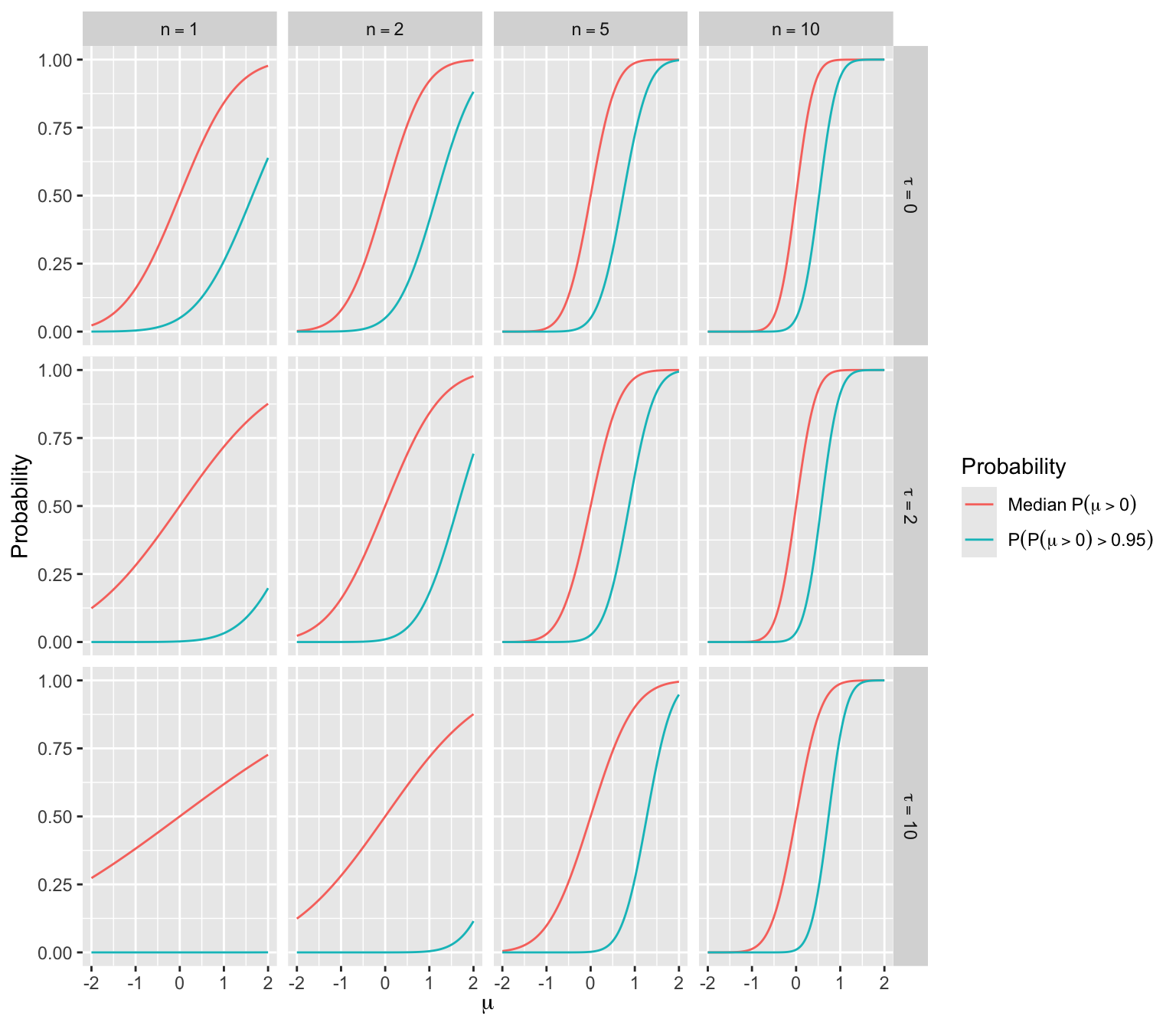
9.7.2 Sample Size for Comparing Time to Event
In this example we compute the sample size needed to achieve adequate Bayesian power to achieve evidence for various assertions. The treatment effect is summarized by a hazard ratio (HR) in a proportional hazards (PH) model. Assertions for which the study needs to have the ability to provide conclusive evidence include
- any reduction of hazard of an event (HR < 1)
- HR < 0.98, 0.96, 0.94, …
- harm or trivial benefit (HR > 0.95)
The trial’s actual analysis might use a flexible parametric PH model implemented in the rstanarm Bayesian survival analysis package. Bayesian operating characteristics are simulated here using the Cox PH model.
Take Bayesian power to be the probability that the posterior probability will exceed 0.975 when the true HR is a constant3. For the first two types of assertions, set the HR generating the data to 0.75 (assumed minimally clinically important difference), and for the third type of assertion set HR to 1.25.
3 Ideally one would consider power over a distribution of HRs as done below.
The actual analysis to be used for the clinical trial should adjust for covariates, but covariates are ignored in our simulations. Bayesian power will increase with the addition of covariates.
If the treatment groups are designated A (standard of care) and B (new treatment), suppose that the following Weibull survival distribution has been found to fit patient’s experiences under control treatment.
\[S(t) = e^{- 0.9357 t^{0.5224}}\] The survival curve for treatment B patients is obtained by multiplying 0.9357 by the B:A hazard ratio (raising \(S(t)\) to the HR power).
Assume further that follow-up lasts 3y, 0.85 of patients will be followed a full 3y, and 0.15 of patients will be followed 1.5y when the final analysis is done4.
4 The R Hmisc package spower function will simulate much more exotic situations.
To compute Bayesian power, use the normal approximation to the Cox partial likelihood function, i.e., assume that log(HR) is normal and use standard maximum likelihood methods to estimate the mean and standard deviation of the log(HR). The Cox log-likelihood is known to be very quadratic in the log HR, so the normal approximation will be very accurate. For a prior distribution assume a very small probability of 0.025 that HR < 0.25 and a probability of 0.025 that it exceeds 4. The standard deviation for log(HR) that accomplishes this is \(\frac{\log(4)}{1.96} = 0.7073 = \sigma\).
With a normal approximation for the data likelihood and a normal prior distribution for log(HR), the posterior distribution is also normal. Let \(\theta\) be the true log(HR) and \(\hat{\theta}\) be the maximum likelihood estimate of \(\theta\) in a given simulated clinical trial. Let \(s\) be the standard error of \(\hat{\theta}\)5.
5 Note that in a proportional hazards model such as the one we’re using, the variance of \(\hat{\theta}\) is very close to the sum of the reciprocals of the event frequencies in the two groups.
Let \(\tau = \frac{1}{\sigma^{2}} = 1.9989\) and let \(\omega = \frac{1}{s ^ {2}}\). Then the approximate posterior distribution of \(\theta\) given the data and the prior is then normal with mean \(\mu\) and variance \(v\) where \(v = \frac{1}{\tau + \omega}\) and \(\mu = \frac{\omega \hat{\theta}}{\tau + \omega}\).
The posterior probability that the true HR < \(h\) is the probability that \(\theta < \log(h)\), which is \(\Phi(\frac{\log(h) - \mu}{\sqrt{v}})\).
Simulation
First consider code for generating outcomes for one clinical trial of size \(n\) per group, follow-up time cutoff \(u\), secondary cutoff time \(u2\) with probability \(pu2\), and true hazard ratio \(H\). The result is posterior mean and variance and the P-value from a frequentist likelihood ratio \(\chi^2\) test with the Cox PH model.
Code
require(data.table)
require(ggplot2)
require(rms)
require(survival)
sim1 <- function(n, u, H, pu2=0, u2=u, rmedian=NA) {
  # n: number of pts in each group
  # u: censoring time
  # H: hazard ratio
  # pu2: probability of censoring at u2 < u
  # rmedian: ratio of two medians and triggers use of log-normal model

  # Generate failure and censoring times for control patients
  # Parameters of a log-normal distribution that resembles the Weibull
  # distribution are below (these apply if rmedian is given)
  mu    <- -0.2438178
  sigma <- 1.5119236

  ta <- if(is.na(rmedian))
    (- log(runif(n)) / 0.9357) ^ (1.0 / 0.5224)
  else exp(rnorm(n, mu, sigma))
  ct <- pmin(u, ifelse(runif(n) < pu2, u2, u))
  ea <- ifelse(ta <= ct, 1, 0)
  ta <- pmin(ta, ct)   # apply censoring
  # Generate failure and censoring times for intervention patients
  tb <- if(is.na(rmedian))
    (- log(runif(n)) / (H * 0.9357)) ^ (1.0 / 0.5224)
  else exp(rnorm(n, mu + log(rmedian), sigma))
  ct <- pmin(u, ifelse(runif(n) < pu2, u2, u))
  eb <- ifelse(tb <= ct, 1, 0)
  tb <- pmin(tb, ct)
  ti <- c(ta, tb)
  ev <- c(ea, eb)
  tx <- c(rep(0, n), rep(1, n))
  f <- if(is.na(rmedian)) coxph(Surv(ti, ev) ~ tx) else
    survreg(Surv(ti, ev) ~ tx, dist='lognormal')
  chi <- 2 * diff(f$loglik)
  theta.hat <- coef(f)[length(coef(f))]
  s2        <- vcov(f)['tx', 'tx']
  tau       <- 1.9989
  omega     <- 1.0 / s2
  v         <- 1.0 / (tau + omega)
  mu        <- omega * theta.hat / (tau + omega)
  if(! all(c(length(mu), length(v), length(chi))) == 1) stop("E")
  list(mu   = as.vector(mu),
       v    = as.vector(v),
       pval = as.vector(1.0 - pchisq(chi, 1)))
}
Simulate all statistics for \(n=50, 51, ..., 1000\) and HR=0.75 and 1.25, with 10 replications per \(n\)/HR combination.
Code
HR <- 0.75
ns <- seq(50, 1000, by=1)
R  <- expand.grid(n = ns, HR=c(0.75, 1.25), rep=1 : 10)
setDT(R)   # convert to data.table
g <- function() {
  set.seed(7)
  R[, sim1(n, 3, HR, 0.15, 1.5), by=.(n, HR, rep)]
  }
S <- runifChanged(g, R, sim1, file='wsim.rds')
Re-run because of changes in the following objects: R The number of trials simulated for each of the two HR’s was 9510.
Before simulating Bayesian power, simulate frequentist power for the Cox PH likelihood ratio \(\chi^2\) test with two-sided \(\alpha=0.05\). Effect size to detect is HR=0.75.
Code
R <- S[HR == 0.75, .(reject = 1 * (pval < 0.05)), by=n]
# Compute moving proportion of trials with p < 0.05
# Use overlapping windows on n and also logistic regression with
# a restricted cubic spline in n with 5 knots
m <- movStats(reject ~  n, eps=100, lrm=TRUE,
              data=R, melt=TRUE)
ggplot(m,
       aes(x=n, y=reject, linetype=Type)) + geom_line() +
  geom_hline(yintercept=0.9, alpha=0.3) +
  scale_x_continuous(breaks=seq(0, 1000, by=100)) +
  scale_y_continuous(breaks=seq(0, 1, by=0.1),
                     minor_breaks=seq(0, 1, by=0.05)) +
  ylab('Pr(reject H0:HR=1)')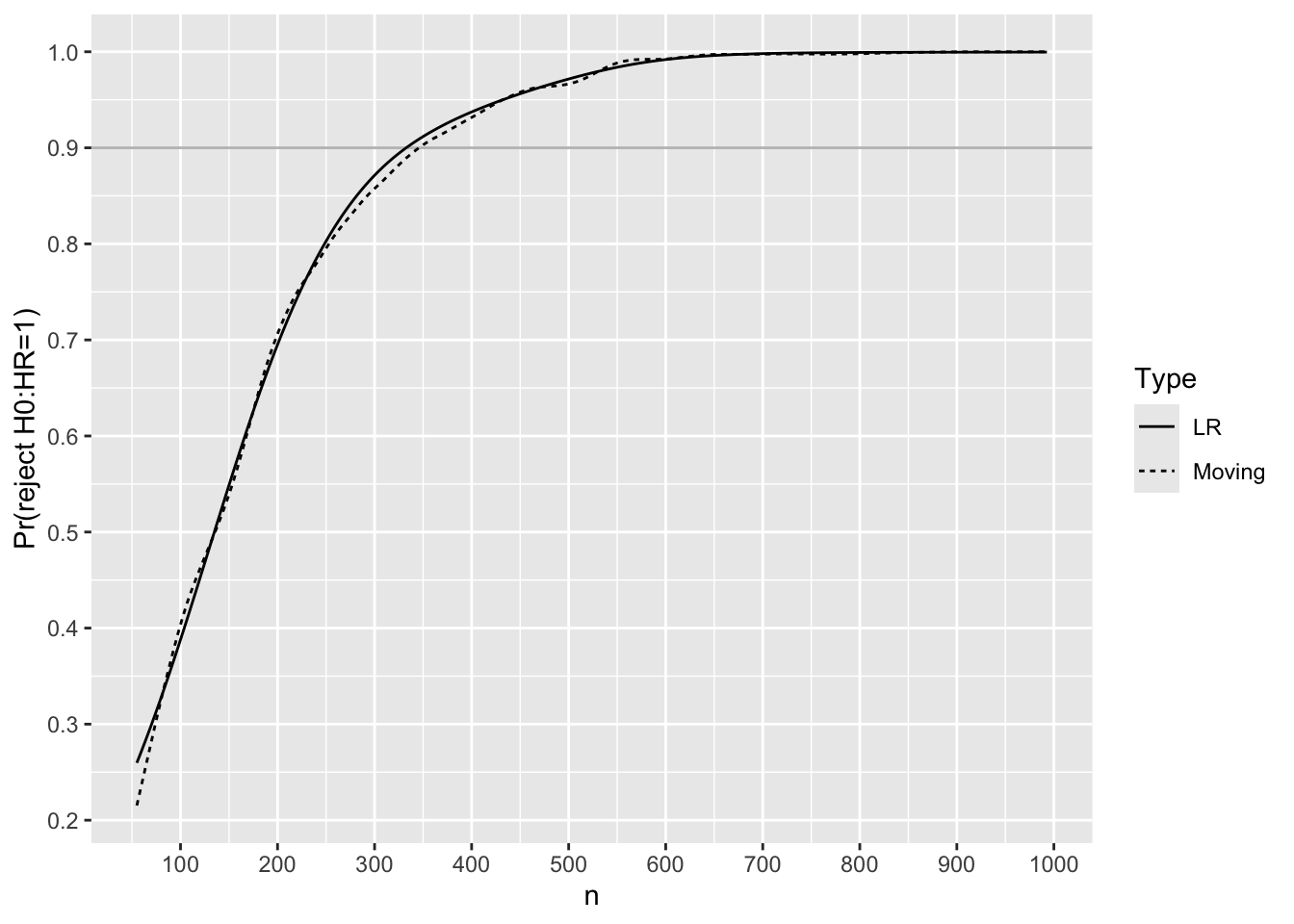
Use linear interpolation to solve for the sample size needed to have 0.9 frequentist power.
Code
lookup <- function(n, p, val=0.9)
  round(approx(p, n, xout=val)$y)
m[Type == 'LR', lookup(n, reject)]
[1] 333For each trial simulated with HR=0.75, compute posterior probabilities that the true HR \(< h\) for various HR cutoffs \(h\). Both moving proportions and logistic regression with a restricted cubic spline in \(n\) are used to smooth the results to estimate the relationship between \(n\) and Bayesian power, i.e., the probability that the posterior probability reaches 0.975 or higher.
Code
R <- S[HR == 0.75]
hs <- seq(0.8, 1.0, by = 0.02)
pp <- function(mu, v) list(h=hs, p=pnorm((log(hs) - mu) / sqrt(v)))
R <- R[, pp(mu, v), by=.(n, rep)]
# Compute moving proportion with posterior prob > 0.975
# with overlapping windows on n, and separately by h
R[, phi := 1 * (p >= 0.975)]
m <- movStats(phi ~  n + h, eps=100, lrm=TRUE, lrm_args=list(maxit=30),
              data=R, melt=TRUE)
ggplot(m,
       aes(x=n, y=phi, color=h, linetype=Type)) + geom_line() +
  geom_hline(yintercept=0.9, alpha=0.3) +
  scale_x_continuous(breaks=seq(0, 1000, by=100)) +
  scale_y_continuous(breaks=seq(0, 1, by=0.1),
                     minor_breaks=seq(0, 1, by=0.05)) +
  ylab('Pr(Posterior Pr(HR < h) > 0.975)')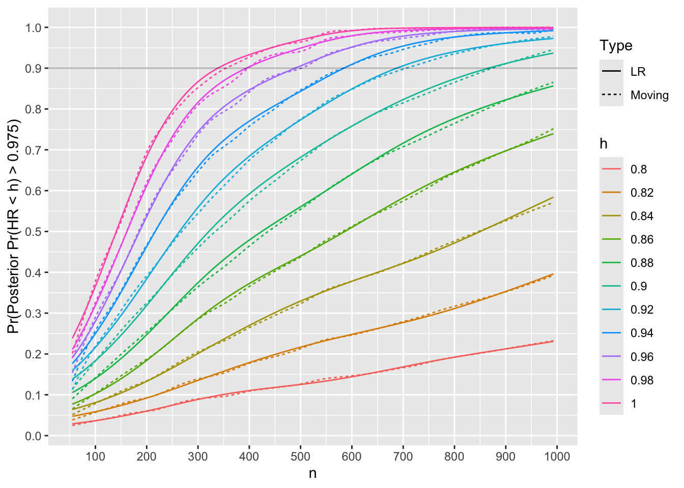
Use linear interpolation to compute the \(n\) for which Bayesian power is 0.9.
Code
u <- m[Type == 'LR', .(nmin=lookup(n, phi)), by=h]
u
h nmin
<char> <num>
1: 0.8 NA
2: 0.82 NA
3: 0.84 NA
4: 0.86 NA
5: 0.88 NA
6: 0.9 866
7: 0.92 687
8: 0.94 584
9: 0.96 489
10: 0.98 394
11: 1 339Code
Nprime <- u[h == 1, nmin]Check the Bayesian power to detect a trivial or worse treatment benefit when true HR is 1.25.
Code
HR <- 1.25
hs <- 0.95
R <- S[HR == 1.25, pp(mu, v), by=.(n, rep)]
# One minus because we want Pr(HR > 0.95)
R[, phi := 1 * (1.0 - p > 0.975)]
m <- movStats(phi ~ n, eps=100, lrm=TRUE, data=R, melt=TRUE,
              lrm_args=list(maxit=30))
ggplot(m, aes(x=n, y=phi, linetype=Type)) + geom_line() +
  ylab('Pr(Posterior Pr(HR > 0.975))') +
  geom_hline(yintercept=0.9, alpha=0.3) +
  scale_x_continuous(breaks=seq(0, 1000, by=100)) +
  scale_y_continuous(breaks=seq(0, 1, by=0.1),
                     minor_breaks=seq(0, 1, by=0.05))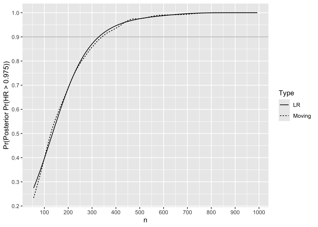
Find \(n\) where it crosses 0.9.
Code
m[Type == 'LR', lookup(n, phi)][1] 328Accounting for Uncertainty in MCID
Different reviewers and journal readers may have different ideas of a minimal clinically important difference to detect. Instead of setting the MCID to HR=0.75, suppose that all HR in the interval [0.65, 0.85] are equally likely to be the MCID at the time the study findings are made known. Let’s re-simulate 1000 trials to compute Bayesian power at a sample size of 339 per group, varying the MCID over [0.65, 0.85].
Code
set.seed(7)
R  <- expand.grid(n = Nprime, HR=runif(1000, 0.65, 0.85))
setDT(R)   # convert to data.table
S <-  R[, sim1(n, 3, HR, 0.15, 1.5), by=.(n, HR)]
pp <- function(mu, v) pnorm((log(1.0) - mu) / sqrt(v))
bp <- S[, mean(pp(mu, v) > 0.975)]
bp
[1] 0.848The Bayesian power drops from 0.9 to 0.848 when the stated amount of uncertainty is taken into account for MCID.
9.7.3 Bayesian Power for 3-Level Ordinal Outcome
Suppose that the above time-to-event outcome is primary, and that there is a secondary outcome of infection within 90 days of randomization. To explicitly account for deaths within the 90-day window we use a 3-level proportional odds ordinal logistic model with 0=alive and infection-free, 1=alive and infection, 2=dead (whether or not preceded by infection). For the actual study we may use a partial proportional odds model to allow for a different treatment effect for the union of infection and death as compared to the effect for death alone. A prior distribution can be specified for the ratio of the two odds ratios (for infection + death and for death) such that there is a 0.95 chance that the ratio of odds ratios is between \(\frac{1}{3}\) and \(3\). A Bayesian power simulation with that amount of borrowing between the treatment effect for the two outcomes is presented at the end of this section.
Use the Weibull model described above to estimate 90-day mortality.
Code
rnd <- function(x) round(x, 3)
S   <- function(t) exp(- 0.9357 * t ^ 0.5224)
m90 <- 1. - S(90 / 365.25)
m30 <- 1. - S(30 / 365.25)
The estimated mortality by 90d is 0.362. The estimated probability of infection for 90-day survivors is 0.2, so the ordinal outcome is expected to have relative frequencies listed in the first line below.
Code
# Hmisc posamsize and popower function cell probabilities are averaged
# over the two groups, so need to go up by the square root of the odds
# ratio to estimate these averages

phigh <- c(1. - 0.2 - m90, 0.2, m90)
or    <- 0.65
pmid  <- pomodm(p=phigh, odds.ratio=sqrt(or))
plow  <- pomodm(p=pmid, odds.ratio=sqrt(or))
phigh <- rnd(phigh)
pmid  <- rnd(pmid)
plow  <- rnd(plow)
n <- round(posamsize(pmid, odds.ratio=or, power=0.8)$n / 2)
Infpow <- round(popower(pmid, odds.ratio=or, n=2 * Nprime)$power, 3)
Infpow
[1] 0.844| Treatment | Y=0 | Y=1 | Y=2 |
|---|---|---|---|
| Standard Tx | 0.438 | 0.2 | 0.362 |
| New Tx | 0.545 | 0.185 | 0.27 |
| Average | 0.491 | 0.195 | 0.314 |
The second line in the table are the outcome probabilities when an odds ratio of 0.65 is applied to the standard treatment probabilities. The last line is what is given to the posampsize and popower functions to compute the sample size need for an \(\alpha=0.05\) two-sided Wilcoxon/proportional odds test for differences in the two groups on the 3-level outcome severity with power of 0.8. The needed sample size is 301 per group were a frequentist test to be used. The frequentist power for the sample size (339 per group) that will be used for the primary outcome is 0.844.
For Bayesian power we use a process similar to what was used for the proportional hazards model above, but not quite trusting the quadratic approximation to the log likelihood for the proportional odds model, due to discretenesss of the outcome variable. Before simulating a power curve for all sample sizes using the normal approximation to the data likelihood, we do a full Bayesian simulation of 1000 trials with 300 patients per group in addition to using the approximate normal prior/normal likelihood method.
Here is a function to simulate one study with an ordinal outcome.
Code
require(rmsb)
options(mc.cores=4, rmsb.backend='cmdstan')
cmdstanr::set_cmdstan_path(cmdstan.loc)

sim1 <- function(n, pcontrol, or, orcut=1, bayes=FALSE) {
  # n: number of pts in each group
  # pcontrol: vector of outcome probabilities for control group
  # or: odds ratio
  # orcut: compute Pr(OR < orcut)

  # Compute outcome probabilities for new treatment
  ptr <- pomodm(p=pcontrol, odds.ratio=or)
  k <- length(pcontrol) - 1
  tx <- c(rep(0, n), rep(1, n))
  y  <- c(sample(0 : k, n, replace=TRUE, prob=pcontrol),
          sample(0 : k, n, replace=TRUE, prob=ptr) )
  f <- lrm(y ~ tx)
  chi <- f$stats['Model L.R.']
  theta.hat <- coef(f)['tx']
  s2        <- vcov(f)['tx', 'tx']
  tau       <- 1.9989
  omega     <- 1.0 / s2
  v         <- 1.0 / (tau + omega)
  mu        <- omega * theta.hat / (tau + omega)
  if(! all(c(length(mu), length(v), length(chi))) == 1) stop("E")

  postprob <- NULL
  if(bayes) {
    # Set prior on the treatment contrast
    pcon <- list(sd=0.7073, c1=list(tx=1), c2=list(tx=0),
                 contrast=expression(c1 - c2) )
    f <- blrm(y ~ tx, pcontrast=pcon,
              loo=FALSE, method='sampling', iter=1000)
    dr <- f$draws[, 'tx']
    postprob <- mean(dr < log(orcut))  # Pr(beta<log(orcut)) = Pr(OR<orcut)
  }
  c(mu   = as.vector(mu),
    v    = as.vector(v),
    pval = as.vector(1.0 - pchisq(chi, 1)),
    postprob = postprob)
}

# Define a function that can be run on split simulations on
# different cores

g <- function() {
  nsim <- 1000
  # Function to do simultions on one core
  run1 <- function(reps, showprogress, core) {
    R <- matrix(NA, nrow=reps, ncol=4,
                dimnames=list(NULL, c('mu', 'v', 'pval', 'postprob')))
    for(i in 1 : reps) {
      showprogress(i, reps, core)
      R[i, ] <- sim1(300, phigh, 0.65, bayes=TRUE)
    }
    list(R=R)
  }
  # Run cores in parallel and combine results
  # 3 cores x 4 MCMC chains = 12 cores = machine maximum
  runParallel(run1, reps=nsim, seed=1, along=1, cores=3)
}
R <- runifChanged(g, file='k3.rds')   # 15 min.
Compute frequentist power and exact (to within simulation error) and approximate Bayesian powper.
Code
u <- as.data.table(R)
pp <- function(mu, v) pnorm((log(1.0) - mu) / sqrt(v))
u[, approxbayes := pp(mu, v)]
cnt <- c(1:5, 10, 25, 50)
ggplot(u, aes(x=approxbayes, y=postprob)) +
  stat_binhex(aes(fill=cut2(after_stat(count), cnt)), bins=75) +
  geom_abline(alpha=0.3) +
  guides(fill=guide_legend(title='Frequency')) +
  xlab('Approximate Posterior Probability OR < 1') +
  ylab('Exact Posterior Probability')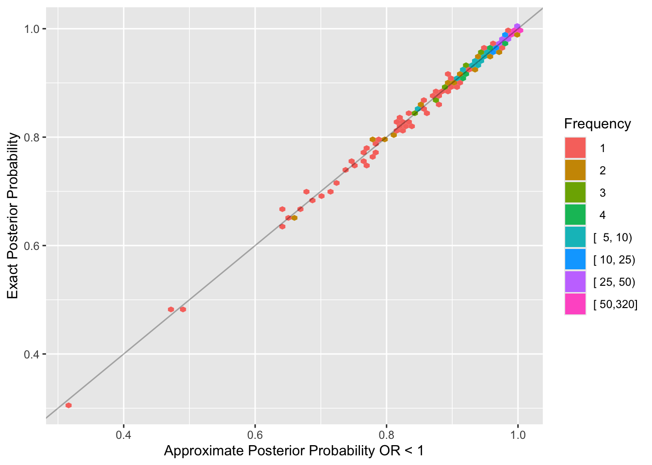
Code
h <- function(x) c(Power = round(mean(x), 3))
u[, rbind('Frequentist'          = h(pval < 0.05),
          'Bayesian'             = h(postprob > 0.975),
          'Approximate Bayesian' = h(approxbayes > 0.975))]
Power
Frequentist 0.795
Bayesian 0.782
Approximate Bayesian 0.780The posterior distribution is extremely well approximated by a normal distribution at a sample size that matters. Bayesian power is just slightly below frequentist power because frequentist test statistics do not place limits on the treatment effect, e.g., allow the odds ratio to be unrealistically far from 1.0.
Use the approximation for proportional odds model Bayesian power going forward. Compute power for the primary endpoint’s sample size.
Code
R  <- expand.grid(n = Nprime, rep=1:1000)
setDT(R)
g <- function() {
  set.seed(17)
  R[, as.list(sim1(n, phigh, or, bayes=FALSE)), by=.(n, rep)]
}
S <- runifChanged(g, R, or, sim1, file='k3n.rds')
Re-run because of changes in the following objects: R Code
S[, pphi := 1 * (pp(mu, v) > 0.975), by=.(n, rep)]
Infpower <- S[, mean(pphi)]
Infpower
[1] 0.811The Bayesian power to detect an OR of 0.65 at a sample size of 339 per group is 0.811.
Bayesian Power for Different Treatment Effect for Infection and Death
The proportional odds (PO) model can provide a correct assessment of which treatment is better overall even when PO is not satisfied. But with non-PO the power will not be optimal, and estimates of outcome probabilities for individual outcomes can be off. To estimate Bayesian power when PO is not assumed, allow the treatment effect (OR) for I|D (infection unioned (“or”d) with death) to differ from the OR for D. In the \(Y=0,1,2\) notation we have one OR for \(Y\geq 1\) and a separate OR for \(Y=2\). This is the partial PO model of Peterson & Harrell (1990). The amount of borrowing for the I|D treatment effect and the D effect is specified by a prior for the ratio of the I|D and D ORs. We assume the log of the ratio of the ORs is normal with mean zero and variance such that the probability that the ratio of ratios is between \(\frac{1}{3}\) and \(3\) is 0.95. The standard deviation accomplishing this is \(\frac{\log(3)}{1.96} = 0.5605\).
Also simulate the power of the treatment comparison on I|D when there is no borrowing of treatment effect information across I and D, i.e., when the prior for the non-PO effect (here the special effect of treatment on D) is non-informative. This partial PO model assumes nothing about how the treatment effect on I|D compares to the effect on D.
The sample size is 302 per group to yield Bayesian power of 0.8 against OR=0.65 in PO holds. For this sample size, simulations showed the loss of power by not assuming PO was minimal when the data satisfied PO. So the simulations are run with \(n=75\) per group to better understand power implications for varying amounts of information borrowing.
The R rmsb package’s blrm function has the user specify priors for departures from PO through contrasts and through a “departure from PO” function (the cppo argument). The contrast for the differential treatment effect over outcome components in the information-borrowing case is the same one that we apply to the main treatment effect except for using a standard deviation involving \(\log(3)\) instead of \(\log(4)\).
When the statistical analysis plan for the study is detailed, more simulations will be run that use a non-PO data generating mechanism, but for now data will be simulated the same as earlier, assuming PO for treatment.
Code
sim1npo <- function(n, pcontrol, or, orcut=1, peffect=FALSE) {
  # n: number of pts in each group
  # pcontrol: vector of outcome probabilities for control group
  # or: odds ratio to detect for I|D
  # orcut: Compute Pr(OR < orcut)
  # Set peffect=TRUE to debug

  # Compute outcome probabilities for new treatment
  ptr <- pomodm(p=pcontrol, odds.ratio=or)
  k <- length(pcontrol) - 1
  tx <- c(rep(0, n), rep(1, n))
  y  <- c(sample(0 : k, n, replace=TRUE, prob=pcontrol),
          sample(0 : k, n, replace=TRUE, prob=ptr) )
  # Set prior on the treatment contrast
  pcon <- list(sd=0.7073, c1=list(tx=1), c2=list(tx=0),
               contrast=expression(c1 - c2) )
  # PO model first
  f <- blrm(y ~ tx, pcontrast=pcon,
            loo=FALSE, method='sampling', iter=1000)
  g <- blrm(y ~ tx,
            y ~ tx, cppo=function(y) y == 2,
            pcontrast=pcon,
            loo=FALSE, method='sampling', iter=1000)

  # Set prior on the "treatment by Y interaction" contrast
  npcon    <- pcon
  npcon$sd <- 0.5605
  h <- blrm(y ~ tx,
            y ~ tx, cppo=function(y) y == 2,
            pcontrast=pcon, npcontrast=npcon,
            loo=FALSE, method='sampling', iter=1000)
  if(peffect) {
    print(f)
    print(g)
    print(h)
    print(rbind(po=c(coef(f), NA), flat=coef(g), skeptical=coef(h)))
    return()
  }
  df <- f$draws[, 'tx']     # log OR for I|D
  dg <- g$draws[, 'tx']     # = log OR for D for PO
  dh <- h$draws[, 'tx']
  # Pr(beta < 0) = Pr(OR < 1)
  lor <- log(orcut)
  c(po = mean(df < lor), flat = mean(dg < lor), skeptical = mean(dh < lor))
}

g <- function() {
  nsim <- 1000
  # Function to do simultions on one core
  run1 <- function(reps, showprogress, core) {
    R <- matrix(NA, nrow=reps, ncol=3,
                dimnames=list(NULL, c('po', 'flat', 'skeptical')))
    for(i in 1 : reps) {
      showprogress(i, reps, core)
      R[i,] <- sim1npo(N, phigh, 0.65)
    }
    list(R=R)
  }
  # Run cores in parallel and combine results
  # 3 cores x 4 MCMC chains = 12 cores = machine maximum
  runParallel(run1, reps=nsim, seed=11, cores=3, along=1)
}
N <- 75
R  <- runifChanged(g, sim1, N, file='k3npo.rds')
bp <- apply(R, 2, function(x) mean(x >= 0.975))
bp
po flat skeptical
0.228 0.203 0.208 For \(n=75\) per group, the Bayesian power is 0.228 when completely borrowing information from D to help inform the treatment effect estimate for D|I. Allowing for arbitrarily different effects (non-PO) reduces the power to 0.203, and assuming some similarity of effects yields a power of 0.208.
9.7.4 Bayesian Power for 6-Level Ordinal Non-Inferiority Outcome
Suppose that the 6-level ECOG performance status assessed at 30 days is another secondary endpoint, and is considered to be a non-inferiority endpoint. Assessment of non-inferiority is more direct with a Bayesian approach and doesn’t need to be as conservative as a frequentist analysis, as we are assessing evidence for a broader range of treatment effects that includes slight harm in addition to the wide range of benefits.
The outcome will be analyzed using a Bayesian proportional odds model with the same prior on the log odds ratio as has been used above. The 6 cell probabilities assumed for the control group appear in the top line in the table below.
The estimated mortality by 30d is 0.224.
Code
# Start with relative probabilities of Y=0-4 and make them
# sum to one minus 30d mortality
phigh <- c(42, 41, 10, 1, 1) / 100
phigh <- c(phigh / sum(phigh) * (1. - m30), m30)
or    <- 0.65
pmid  <- pomodm(p=phigh, odds.ratio=sqrt(or))
plow  <- pomodm(p=pmid, odds.ratio=sqrt(or))
n     <- round(posamsize(pmid, odds.ratio=or, power=0.8)$n / 2)
Perfpowf <- popower(pmid, odds.ratio=or, n = Nprime * 2)$power
g <- function(x) {
  names(x) <- paste0('Y=', (1 : length(x)) - 1)
  round(x, 3)
}
rbind('Standard treatment' = g(phigh),
      'New treatment'      = g(plow),
      'Average'            = g(pmid) )
Y=0 Y=1 Y=2 Y=3 Y=4 Y=5
Standard treatment 0.343 0.335 0.082 0.008 0.008 0.224
New treatment 0.446 0.319 0.065 0.006 0.006 0.158
Average 0.393 0.330 0.074 0.007 0.007 0.189The second line in the table are the outcome probabilities when an odds ratio of 0.65 is applied to the standard treatment probabilities. The last line is what is given to the posampsize function to compute the sample size need for an \(\alpha=0.05\) two-sided Wilcoxon / proportional odds test for differences in the two groups on the 6-level outcome severity with power of 0.8. This is also used for popower. The needed sample size is 283 per group were a frequentist test to be used. This is for a superiority design. The frequentist power for 339 per group is 0.864524.
For performance status a non-inferiority design is used, so Bayesian power will differ more from frequentist superiority power, as the Bayesian posterior probability of interest is \(P(\text{OR} < 1.2)\). Simulate Bayesian power using the normal approximation.
Code
g <- function() {
  set.seed(14)
  or <- 0.65
  R  <- expand.grid(n = Nprime, rep=1:1000)
  setDT(R)
  R[, as.list(sim1(n, phigh, or, orcut=1.2, bayes=FALSE)), by=.(n, rep)]
}
S <- runifChanged(g, sim1, file='k6.rds')   # 16s
pp <- function(mu, v) pnorm((log(1.2) - mu) / sqrt(v))
S[, pphi := 1 * (pp(mu, v) > 0.975), by=.(n, rep)]
Perfpowb <- S[, mean(pphi)]
Bayesian power to detect an OR of 0.65 when seeking evidence for OR < 1.2 with 339 patients per group is 0.987.
9.8 Sample Size Needed For Prior Insensitivity
One way to choose a target sample size is to solve for \(n\) that controls the maximum absolute difference in posterior probabilities of interest, over the spectrum of possible-to-observe data. Let
- \(n\) = sample size in each of two treatment groups
- \(\Delta\) = unknown treatment effect expressed as a difference in means \(\mu_{1} - \mu_{2}\)
- the data have a normal distribution with variance 1.0
- \(\hat{\Delta}\) = observed difference in sample means \(\overline{Y}_{1} - \overline{Y}_{2}\)
- \(V(\hat{\Delta}) = \frac{2}{n}\)
- Frequentist test statistic: \(z = \frac{\hat{\Delta}}{\sqrt{\frac{2}{n}}}\)
- \(\delta\) assumed to be the difference not to miss, for frequentist power
- One-sided frequentist power for two-sided \(\alpha\) with \(z\) critical value \(z_{\alpha}\): \(P(z > z_{\alpha}) = 1 - \Phi(z_{\alpha} - \frac{\delta}{\sqrt{\frac{2}{n}}})\)
Power curves are shown below for \(\alpha=0.05\).
Code
d <- expand.grid(n=c(1:19, seq(20, 200, by=5)),
                 delta = seq(0, 2, by=0.25))
ggplot(d, aes(x=n, y=1 - pnorm(qnorm(0.975) - delta / sqrt(2 / n)), color=factor(delta))) +
  geom_line() + guides(color=guide_legend(title=expression(delta))) +
  scale_x_continuous(minor_breaks=seq(0, 200, by=10)) +
  scale_y_continuous(minor_breaks=seq(0,   1, by=0.05)) +
  xlab('n') + ylab(expression(paste('Power at ', alpha==0.05)))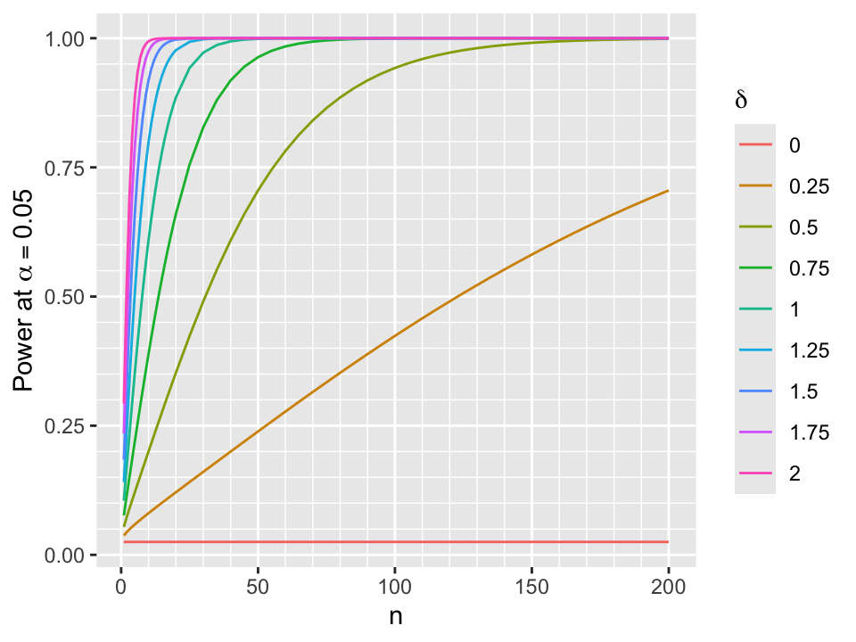
- Assume skeptical prior for \(\Delta\) that is normal with mean 0 and variance \(\frac{1}{\tau}\)
- Posterior distribution for \(\Delta | \hat{\Delta}\) is normal
- variance = \(\frac{1}{\tau + \frac{n}{2}}\)
- mean = \(\frac{n\hat{\Delta}}{n + 2\tau}\)
Code
pp <- function(tau, n, delta, Deltahat)
  round(1 - pnorm((delta - n * Deltahat / (n + 2 * tau)) * sqrt(tau + n / 2)), 4)
# Compute prior SD such that P(Delta > delta) = prob
psd <- function(delta, prob) round(delta / qnorm(1 - prob), 4)- Example: Probability of misleading evidence for efficacy
- agreed-upon prior was such that \(P(\Delta > 0.5) = 0.05 \rightarrow\) SD of the prior is 0.304
- someone disagrees, and has their own posterior probability of efficacy based on their prior, which was chosen so that \(P(\Delta > 0.5) = 0.005 \rightarrow\) SD of their prior is 0.1941
- suppose that \(\hat{\Delta}\) at \(n=100\) is 0.3
- \(\rightarrow\) posterior probability of \(\Delta > 0\) using pre-specified prior is 0.9801
- \(\rightarrow\) posterior probability of \(\Delta > 0\) using the critic’s prior is 0.9783
- there is substantial evidence for efficacy in the right direction
- probability of being wrong in acting as if the treatment works is 0.0199 to those who designed the study, and is 0.0217 to the critic
- the two will disagree more about evidence for a large effect, e.g. \(P(\Delta > 0.2)\)
- \(P(\Delta > 0.2)\) using pre-specified prior: 0.724
- \(P(\Delta > 0.2)\) for the critic: 0.7035
- Probabilities of being wrong in acting as if the treatment effect is large: 0.276, 0.2965
- Sample size needed to overcome effect of prior depends on the narrowness of the prior (\(\tau; \sigma\))
- for posterior mean and variance to be within a ratio \(r\) of those from a flat prior \(n\) must be \(> \frac{2\tau r}{1 - r}\)
- within 5% for \(n > 38\tau\)
- within 2% for \(n > 98\tau\)
- within 1% for \(n > 198\tau\)
- typical value of \(\sigma = \frac{1}{\tau} = 0.5\) so \(n > 196\) to globally be only 2% sensitive to the prior
- Posterior \(P(\Delta > \delta | \hat{\Delta}) = 1 - \Phi((\delta - \frac{n\hat{\Delta}}{n + 2\tau})\sqrt{\tau + \frac{n}{2}})\)
- Choose different values of the prior SD to examine sensitivity of cumulative posterior distribution to prior
- Below see that the posterior probability of any treatment benefit (when \(\delta=0\)) is not sensitive to the prior
- Probability of benefit \(> \delta\) for large \(\delta\) is sensitive to the prior
- priors having large probability of large \(\Delta\) lead to higher posterior probabilities of large \(\Delta > \delta\) when \(\delta\) is large
- For each \(n, \delta\), and SDs compute the absolute difference in posterior probabilities that \(\Delta > \delta\)
- First look at the result when assessing evidence for any efficacy (\(\delta=0\)) when the most extreme priors (\(\sigma=\frac{1}{8}\) vs. \(\sigma=8\)) are compared
- Don’t consider conditions when both posterior probabilities are in [0.1, 0.9] where disagreements are probably inconsequential
Code
require(data.table)
sigmas <- c(1/8, 8)
w <- expand.grid(n        = c(1:30, seq(35, 200, by=5)),
                 Deltahat = seq(-1, 5, by=0.025))
setDT(w)
z <- lapply(1 : nrow(w),
            function(i) w[i, .(n, Deltahat,
                               p1 = pp(8,   n, 0, Deltahat),
                               p2 = pp(1/8, n, 0, Deltahat) )] )
u <- rbindlist(z)
# Ignore conditions where both posterior probabilities are in [0.1, 0.9]
# Find maximum abs difference over all Deltahat
m <- u[, .(mdif = max(abs(p1 - p2) * (p1 < 0.1 | p2 < 0.1 | p1 > 0.9 | p2 > 0.9))), by=n]
ggplot(m, aes(x=n, y=mdif)) + geom_line() +
  scale_x_continuous(minor_breaks=seq(0, 200, by=10)) +
  scale_y_continuous(minor_breaks=seq(0, 0.2, by=0.01)) +
  ylab(expression(paste('Maximum |Difference| in ', Pr(Delta > delta ~ "|" ~ hat(Delta)))))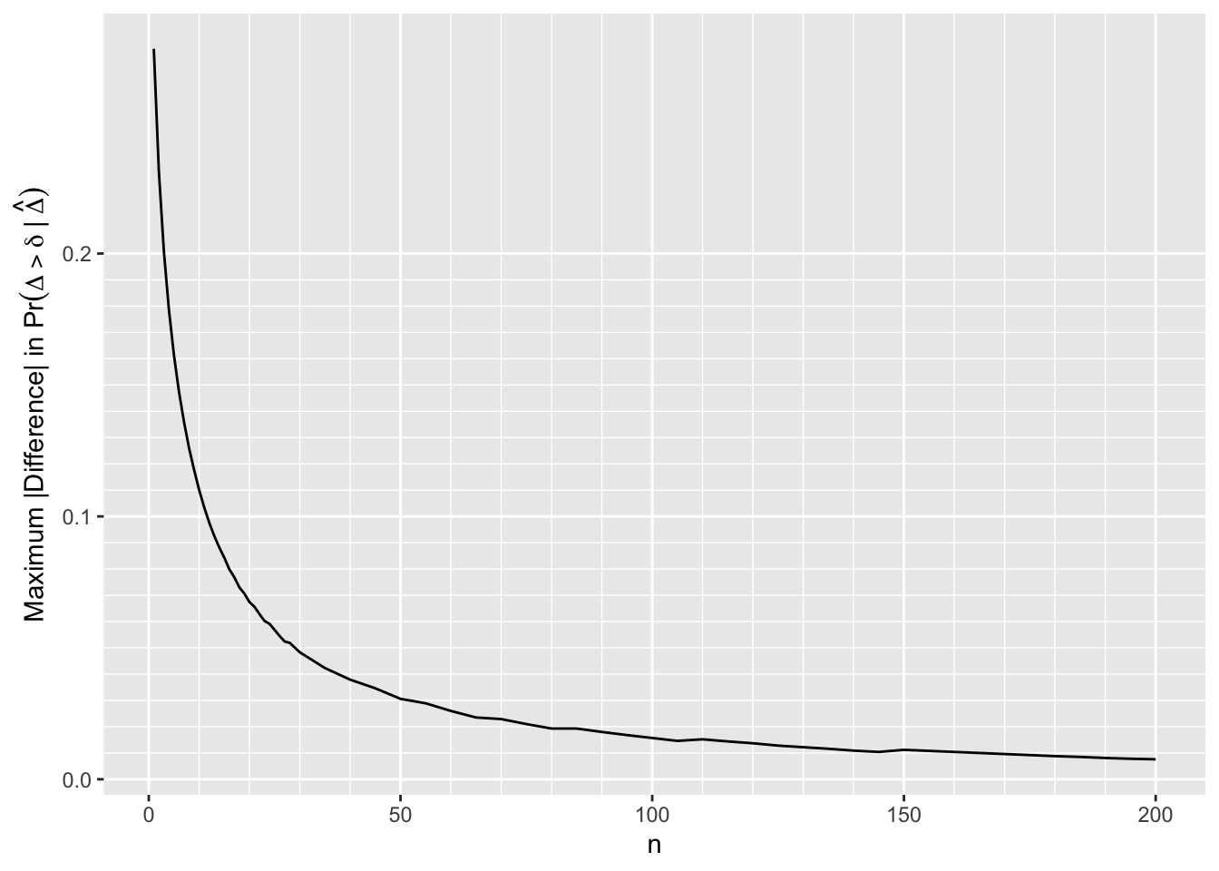
By \(n=170\) the largest absolute difference in posterior probabilities of any efficacy is 0.01
The difference is 0.02 by \(n=80\)
Sample sizes needed for frequentist power of 0.9 are \(n=38\) for \(\Delta=0.5\) and \(n=85\) for \(\Delta=0.25\)
Now consider the full picture where evidence for efficacy \(> \delta\) where \(\delta \neq 0\) is included
Vary \(n, \delta, \hat{\Delta}\) and the two prior SDs
Don’t show points where the difference < 0.0025 or when both posterior probabilities are in [0.1, 0.9]
In the graph one of the prior SDs is going across, and the other is vertical; diagonals where the two SDs are equal are not needed
Code
# For a given n and delta two values of SDs compute the absolute difference
# of the two posterior probabilities that Delta > delta when one of the posterior
# probabilities was < 0.1 or > 0.9 and when the difference exceeds 0.0025
adif <- function(n, delta, s1, s2) {
  tau1 <- 1 / s1
  tau2 <- 1 / s2
  Deltahat <- seq(-1, 5, by=0.05)
  p1 <- pp(tau1, n, delta, Deltahat)
  p2 <- pp(tau2, n, delta, Deltahat)
  i  <- abs(p1 - p2) >= 0.0025 & (pmin(p1, p2) < 0.1 | pmax(p1, p2) > 0.9)
  data.table(n, delta, s1, s2, Deltahat, ad=abs(p1 - p2))[i]
}
taus <- c(1/8, 1/4, 1/2, 1, 2, 4, 8)
sigmas <- 1 / taus
dels   <- seq(-1, 1, by=0.5)
w <- expand.grid(n     = c(10, 15, seq(20, 400, by=10)),
                 delta = dels,
                 s1    = sigmas,
                 s2    = sigmas)
setDT(w)
w <- w[s2 > s1]
z <- lapply(1 : nrow(w), function(i) w[i, adif(n, delta, s1, s2)])
u <- rbindlist(z)
u[, adc := cut2(ad, c(0, 0.005, 0.01, 0.02, 0.03, 0.04, 0.05, 0.075, 0.1, 0.15, 0.2, 0.4))]
g <- vector('list', length(dels))
names(g) <- paste0('δ=', dels)
for(del in dels)
  g[[paste0('δ=', del)]] <- ggplot(u[delta==del], aes(x=n, y=Deltahat, color=adc)) + geom_point(size=0.3) +
    facet_grid(s1 ~ s2) + guides(color=guide_legend(title='|Difference|')) +
    theme(legend.position='bottom') +
    ylab(expression(hat(Delta))) +
    labs(caption=bquote(delta == .(del)))
maketabs(g, initblank=TRUE)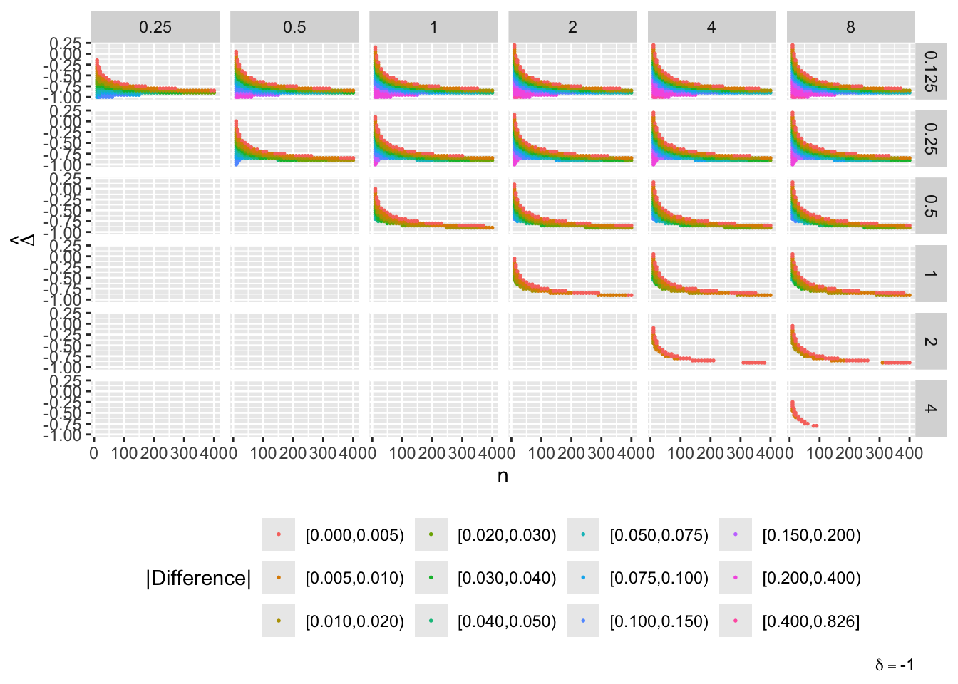
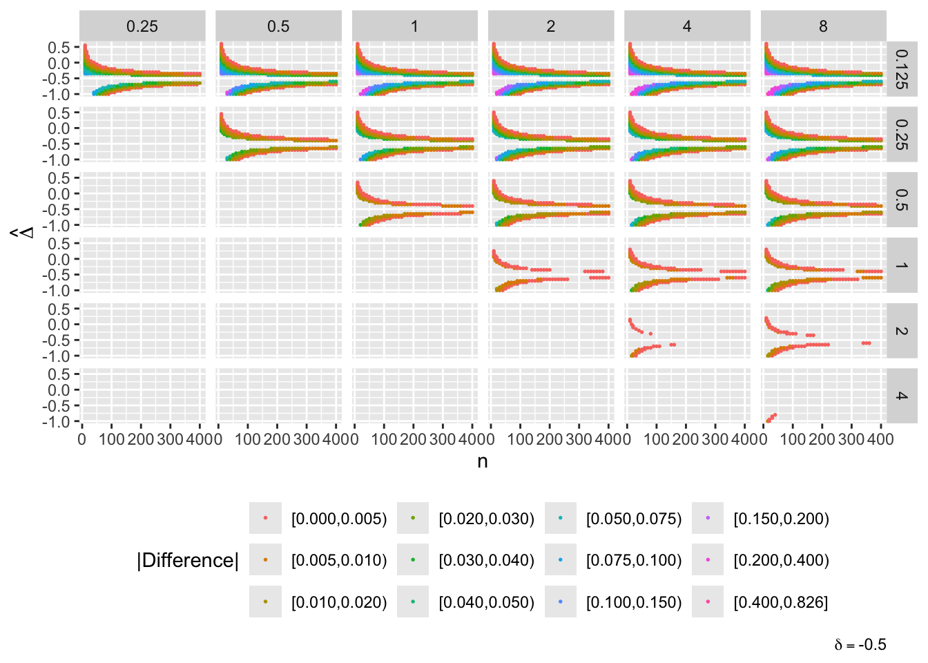
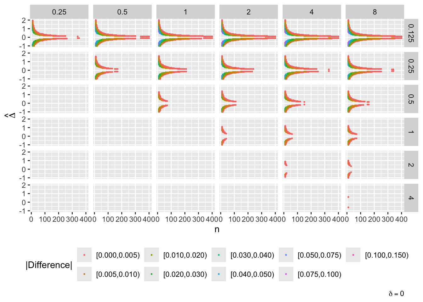
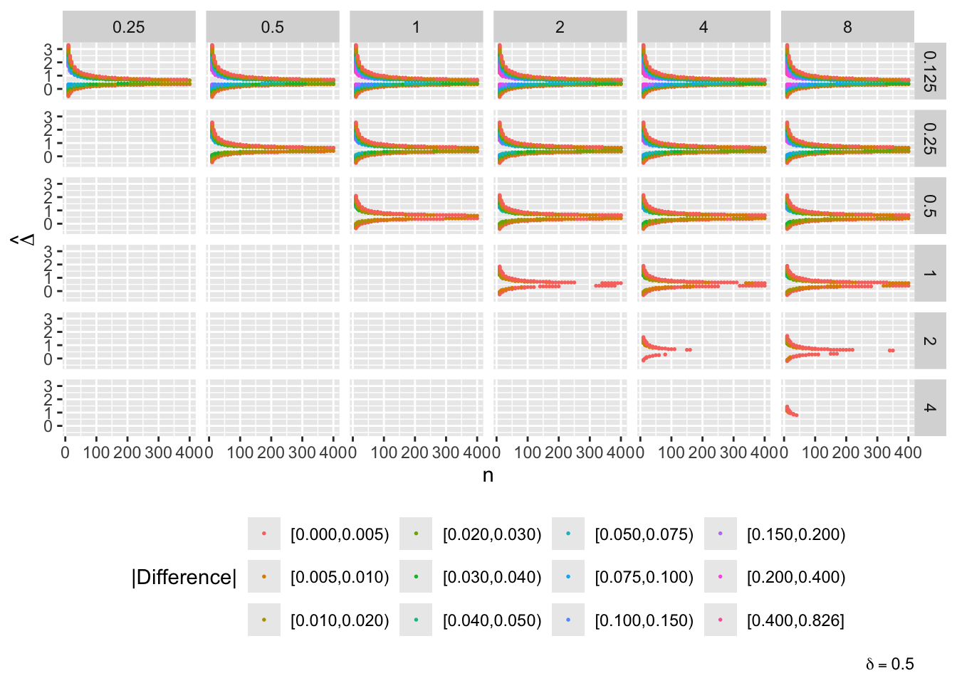
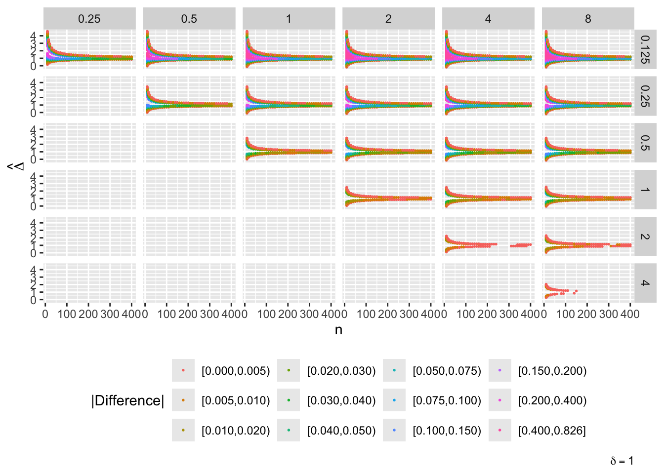
- “Mouth” from the left of each panel corresponds to regions where both posterior probabilities are in [0.1, 0.9]
- Most extremely different priors examined had SD=0.25 (skeptical of large \(\Delta\)) vs. SD=8 (large \(\Delta\) are likely)
- For \(\delta=0\) differences vanish for \(n > 200\)
- For \(\delta=-1\) differences are greatest when observed differences in means \(\hat{\Delta} = -1\)
- For \(\delta=1\) differences are greatest when \(\hat{\Delta} = 1\)
- Required \(n=400\) for influence of prior to almost vanish everywhere when the most different priors are paired
- More realistic to compare somewhat skeptical SD=1 with skeptical SD=0.25
- Larger discrepancy when \(\delta=-1\) and \(\hat{\Delta}=-1\)
- \(n > 300\) makes for small discrepancy
Another display of the same conditions except for fewer values of \(\hat{\Delta}\).
Code
w <- expand.grid(n        = c(10, 15, seq(20, 400, by=10)),
                 delta    = seq(-1, 1, by=0.5),
                 s        = sigmas,
                 Deltahat = c(-1, -0.5, 0, 0.25, 0.5, 0.75, 1, 1.5))
setDT(w)
z <- lapply(1 : nrow(w), function(i) w[i, .(n, delta, s, Deltahat, pp=pp(1/s, n, delta, Deltahat))])
u <- rbindlist(z)
ggplot(u, aes(x=n, y=pp, color=factor(s))) + geom_line() +
  facet_grid(paste0('delta==', delta) ~ paste('hat(Delta)==', Deltahat), label='label_parsed') +
  guides(color=guide_legend(title=expression(paste('Prior ', sigma)))) +
  ylab(expression(Pr(Delta > delta ~ "|" ~ hat(Delta)))) +
  theme(legend.position='bottom')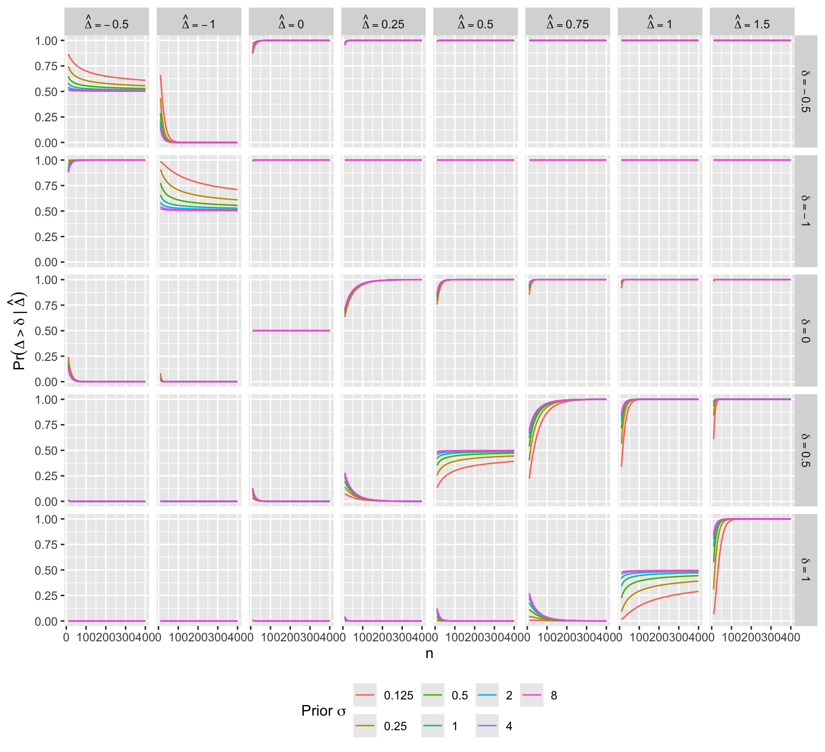
See Rigat (2023) for related ideas.
9.9 Sequential Monitoring and Futility Analysis
I want to make it quite clear that I have no objection with flexible designs where they help us avoid pursuing dead-ends. The analogous technique from the sequential design world is stopping for futility. In my opinion of all the techniques of sequential analysis, this is the most useful. — Senn (2013)
- Compute PP as often as desired, even continuously
- Formal Bayesian approach can also consider having adequate safety data
- Stop when PP > 0.95 for any efficacy and PP > 0.95 for safety event hazard ratio ≤ 1.2
- Spiegelhalter et al. (1993) argue for use of ‘range of equivalence’ in monitoring
- Bayesian design is very simple if no cap on n
- But often reach a point where clinically important efficacy unlikely to be demonstrated within a reasonable n
- Futility is more easily defined with Bayes. 3 possible choices:
- Stop when P(efficacy < ε) is > 0.9
- Use posterior predictive distribution at planned max sample size (Berry (2006))
- Pre-specify max n and continue until that n if trial not stopped early for efficacy or harm (more expensive)
- Insightful approximation of Spiegelhalter et al. (1993)
- use Z-statistic at an interim look
- assume fraction f of subjects randomized to date
- based only on observables
Code
spar(bty='l')
pf <- function(z, f) pnorm(z/sqrt(1 - f) - 1.96 * sqrt(f) / sqrt(1 - f))
zs <- seq(-1, 3, length=200)
fs <- c(.1, .25, .4, .75, .9)
d <- expand.grid(Z=zs, f=fs)
f <- d$f
d$p <- with(d, pf(Z, f))
d$f <- NULL
p <- split(d, f)
labcurve(p, pl=TRUE, ylab='Predictive Probability')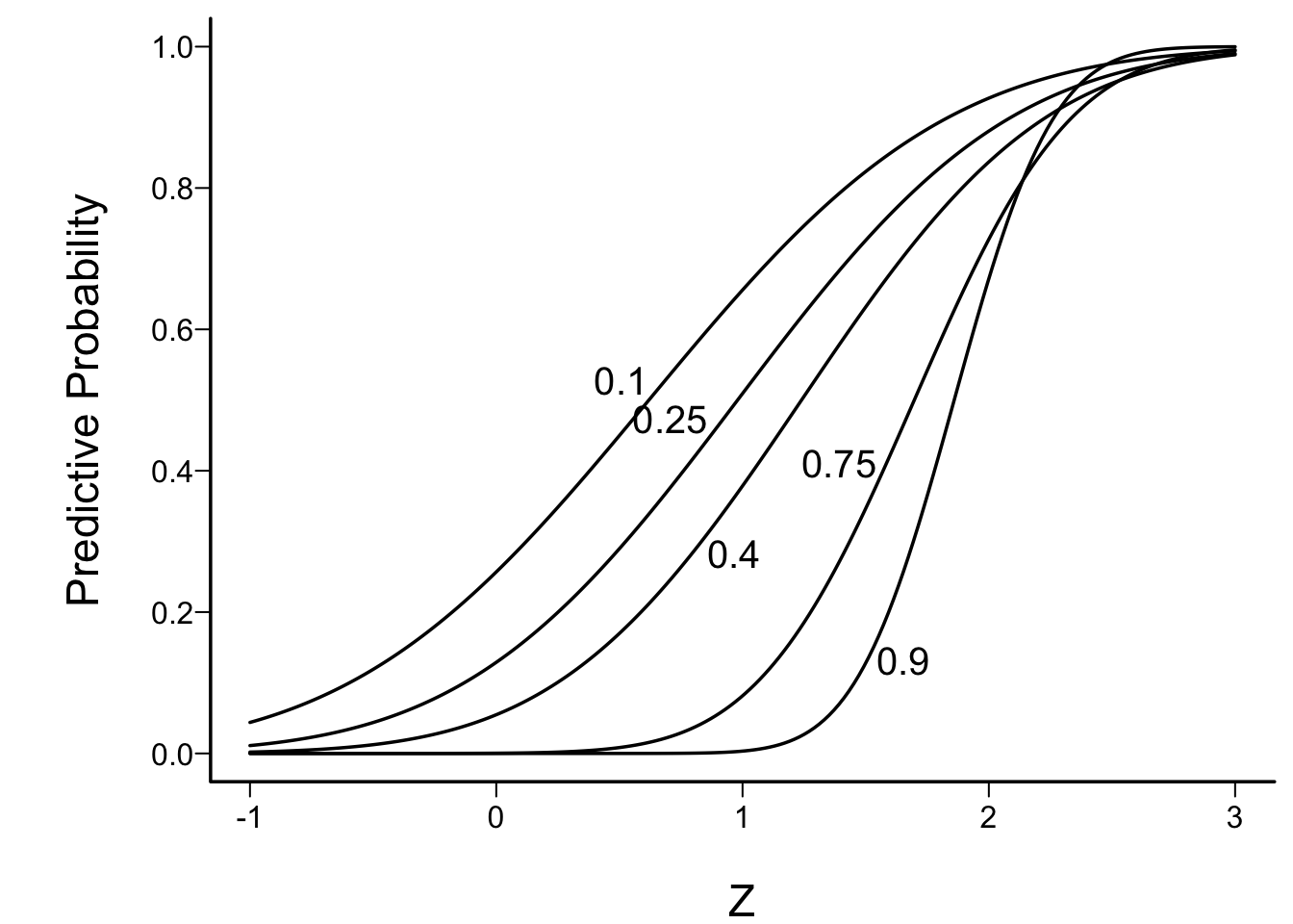
Example: to have reasonable hope of demonstrating efficacy if an interim Z value is 1.0, one must be less than 1/10th of the way through the trial
For example simulations of futility see this
The published report of any study attempts to answer the crucial question: What does this trial add to our knowledge? The strength of the Bayesian approach is that it allows one to express the answer formally. It therefore provides a rational framework for dealing with many crucial issues in trial design, monitoring and reporting. In particular, by making explicitly different prior opinions about efficacy, and differing demands on new therapies, it may shed light on the varying attitudes to balancing the clinical duty to provide the best treatment for individual patients, against the desire to provide sufficient evidence to convince the general body of clinical practice. — Spiegelhalter et al. (1993)
9.10 Example Operating Characteristics
Even with a disadvantageous mismatch between the prior used in the analysis and the prior used to generate the universe of efficacies, the design was able to stop early for evidence of non-trivial efficacy in 0.401 of 10,000 trials over a skeptical distribution of true efficacies, and was right 0.91 of the time when doing so. The design was right 0.98 of the time in terms of there being truly some efficacy when stopping for more than trivial efficacy. Stopping early for evidence of less than trivial efficacy was possible in 0.518 of the trials and was the correct decision 0.97 of the time. One quarter of such trials stopped with fewer than 14 participants studied and half had a sample size less than 32. Overall the average sample size at the time of stopping was 138 for the most skeptical prior, which is just over ½ what a traditional frequentist design would require (234) just to have power to detect the MCID, still not providing evidence for non-trivial efficacy, inefficacy, or similarity. With the Bayesian sequential design only 0.024 of the trials ended without a conclusion for the most skeptical prior.
For the Bayesian sequential design at the start of this chapter, simulate the operating characteristics for the following setting.
- Two-arm parallel-group RCT with equal sample sizes per group
- Response variable is normal with standard deviation 1.0
- Estimand of interest is \(\Delta\) = the unknown difference in means
- MCID is \(\delta=0.3\)
- Minimum clinically detectable difference is \(\gamma=0.1\)
- Similarity interval is \(\Delta \in [-0.15, 0.15]\)
- Maximum affordable sample size is 750 per treatment group
- Required minimum precision in estimating \(\Delta\): \(\pm 0.4\) (half-width of 0.95 credible interval)
- \(\rightarrow\) minimum sample size \(N_{p}\) before stopping for efficacy
- Allow stopping for inefficacy at any time, even if the treatment effect cannot be estimated after stopping, i.e., one only knows there is a high probability that the effect \(< \gamma\).
- The first analysis takes place after the first participant has been enrolled and followed, then after each successive new participant’s data are complete. The first look for efficacy is delayed until the \(N_{p}^\text{th}\) participant has been followed so that the magnitude of the treatment effect has some hope of being estimated.
- Prior for \(\Delta\) is normal with mean 0 and SD \(\sigma\) such that \(P(\Delta > 0.75) = \kappa\) where \(\kappa\) is varied over \({0.2, 0.1, 0.05, 0.025}\)
- This corresponds to \(\sigma=\) 0.8911, 0.5852, 0.456, 0.3827
- These are skeptical priors, chosen because the treatment is assumed to be an incremental rather than a curative therapy
With these similarity limits a large number of studies were stopped early for similarity. In one test with a narrower similarity interval, 0.035 of simulated studies were stopped early for similarity.When using an ultra-high information continuous response variable as in this example, with the between-subject standard deviation known to be 1.0, the data having a normal distribution, and not delaying the first look, it is possible to make a decision with any one participant if she has a very impressive response. This could never happen with a binary endpoint or with unknown SD.
The assumed data model leads to a frequentist point estimate of \(\Delta\) = \(\hat{\Delta}\) = difference in two means, with variance \(\frac{2}{n}\), where \(n\) is the per-group sample size. The one-sided frequentist power for a two-tailed test with \(\alpha=0.05\) is \(1 - \Phi(1.96 - \frac{0.3}{\sqrt{\frac{2}{n}}})\), and setting this to 0.9 requires \(n=2[\frac{1.96 + 1.282}{0.3}]^2 = 234\). 1.282 is \(\Phi^{-1}(0.9)\).
To arrive at \(N_{p}\), the minimum sample size needed to achieve non-embarrassing precision in estimating \(\Delta\), keep in mind that skeptical priors for \(\Delta\) push the posterior distribution for \(\Delta\) towards zero, resulting in narrower posterior distributions. To be conservative in estimating \(N_{p}\) use a flat prior. The 0.90 credible interval is \(\hat{\Delta} \pm 1.645\sqrt{\frac{2}{n}}\). Setting the half-length of the interval to \(\delta=0.3\) results in \(n = N_{p} = 2(\frac{1.645}{0.3})^2 = 60\) per group.
Were a margin of error of 0.2 been required, \(N_{p}=135\), i.e., the first look for possible stoppage for efficacy would be at the \(135^\text{th}\) participant. Setting the required precision to 0.085 would result in no early stopping for efficacy, which is a choice that some trial designers may make, but it requires massive justification for the choice of the maximum sample size.
At a given interim look with a cumulative difference in means of \(\hat{\Delta}\) the posterior distribution of \(\Delta | \hat{\Delta}\) is normal with variance \(\frac{1}{\tau + \frac{n}{2}}\) and mean \(\frac{n\hat{\Delta}}{n + 2\tau}\) where \(\tau\) is the prior precision, \(\frac{1}{\sigma^2}\). Here is a function to compute the posterior probability that \(\Delta > \delta\) given the current difference in means \(\hat{\Delta}\).
Code
pp <- function(delta, Deltahat, n, kappa) {
  sigma <- psd(0.75, kappa)
  tau   <- 1. / sigma ^ 2
  v     <- 1. / (tau + n / 2.)
  m     <- n * Deltahat / (n + 2. * tau)
  1. - pnorm(delta, m, sqrt(v))
}
A simple Bayesian power calculation for a single analysis after \(n\) participants are enrolled in each treatment group, and considering only evidence for any efficacy, sets the probability at 0.9 that the posterior probability of \(\Delta > 0\) exceeds 0.95 when \(\Delta=\delta\). The posterior probability PP that \(\Delta > 0\) is \(\Phi(\frac{n\hat{\Delta}/\sqrt{2}}{\sqrt{n + 2\tau}})\). Making use of \(\hat{\Delta} \sim n(\delta, \frac{2}{n})\), the probability that PP > 0.95 is \(1 - \Phi(\frac{za - \delta}{\sqrt{\frac{2}{n}}})\) where \(z = \Phi^{-1}(0.95)\) and \(a=\frac{\sqrt{2}\sqrt{n + 2\tau}}{n}\).
Code
# Special case when gamma=0, for checking
bpow <- function(n, delta=0.3, kappa=0.05) {
  tau <- 1. / psd(0.75, kappa) ^ 2
  z <- qnorm(0.95)
  a <- sqrt(2) * sqrt(n + 2 * tau) / n
  1. - pnorm((z * a - delta) / sqrt(2 / n))
}
bpow <- function(n, delta=0.3, gamma=0, kappa=0.05, ppcut=0.95) {
  tau <- 1. / psd(0.75, kappa) ^ 2
  z <- qnorm(ppcut)
  a <- n + 2. * tau
  1. - pnorm(sqrt(n / 2) * ((a / n) * (gamma + z * sqrt(2 / a) ) - delta))
}
findx <- function(x, y, ycrit, dec=0) round(approx(y, x, xout=ycrit)$y, dec)
R$bayesN <- round(findx(10:500, bpow(10:500), 0.9))
bpow(R$bayesN)
[1] 0.9006247Setting the Bayesian power to 0.9 results in \(196\) when \(\kappa=0.05\). Contrast this with the frequentist sample size of 234.
To understand the stringency of adding the requirement that efficacy is non-trivial to the requirement of having a very high probability that any efficacy exists, consider a sample size (45) and current mean difference (0.3) where the probability of any efficacy is 0.9. Compute the probability of non-trivial efficacy with that mean difference. The prior probability of a very large (0.75) or larger treatment effect is taken as \(\kappa=0.05\).
Code
pp( 0, 0.3, 45, 0.05)[1] 0.9017632Code
pp(0.1, 0.3, 45, 0.05)[1] 0.7790777Code
pp( 0, 0.36, 45, 0.05)[1] 0.9394288Code
pp(0.1, 0.36, 45, 0.05)[1] 0.8478874At the point at which there is over 0.9 chance of any efficacy in the right direction, the probability of non-trivial efficacy is 0.78. To achieve a probability of 0.85 would require an observed mean difference of 0.36 which raises the probability of any efficacy to 0.94.
What if instead we wanted 0.9 Bayesian power to achieve a PP > 0.85 that \(\Delta > \gamma\), the threshold for a detectable treatment effect? Let’s compute over a range of \(n\) the two relevant probabilities: of getting \(P(\Delta > 0) > 0.95\) and of getting \(P(\Delta > 0.10) >0.85\), and also compute Bayesian power for \(P(\Delta > 0.15) > 0.8\).
Code
gammas <- c(0,      .1, .15)
ppcuts <- c(0.95, 0.85, 0.8)
w <- expand.grid(crit=1:3, n=seq(10, 750, by=5))
setDT(w)
w[, Criterion := paste0('Pr(efficacy > ', gammas[crit], ') > ', ppcuts[crit])]
w[, p := bpow(n=n, gamma=gammas[crit], ppcut=ppcuts[crit])]
ggplot(w, aes(x=n, y=p, col=Criterion)) + geom_line() +
  scale_y_continuous(breaks=seq(0, 1, by=0.1)) +
  ylab('Bayesian Power') +
  theme(legend.position='bottom')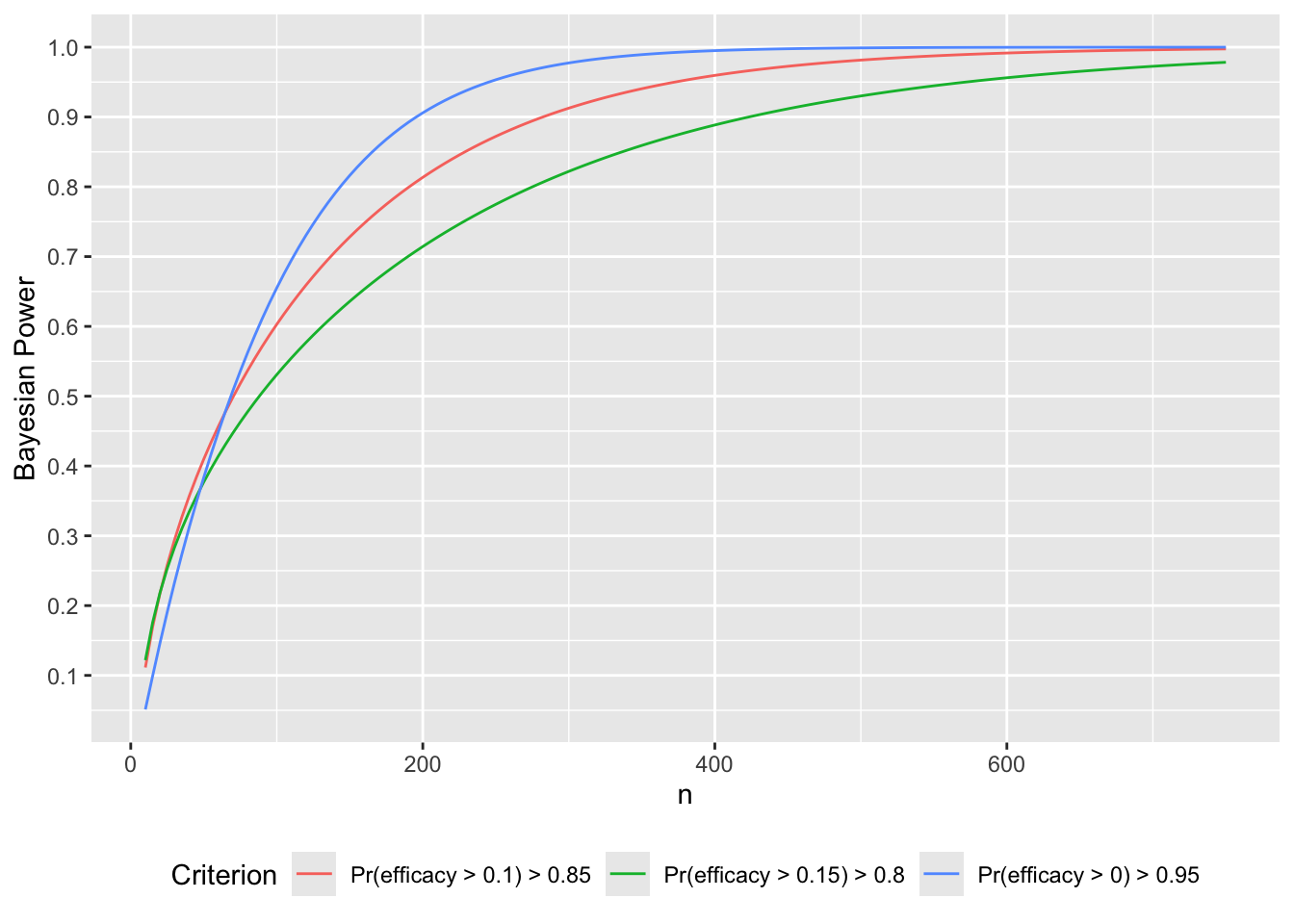
Code
# Solve for n to get Bayesian power of 0.9
p <- w[, .(n=findx(n, p, 0.9)), by=.(crit, Criterion)]
navg <- if(length(R$stopn))
  R$stopn[conclusion == 'non-trivial efficacy' & kappa==0.001, Mean]
For a fixed sample-size study the necessary \(N\) to have a 0.9 chance that the posterior probability of more than trivial efficacy exceeds 0.85 is 282.
Later in this section the expected sample size to establishment of non-trivial efficacy will be estimated when continuous sequential analysis is allowed. This number is 122 for the most skeptical prior used. The more general expected sample size is that required on the average to reach any conclusion. This number is 138.
9.10.1 Decision Thresholds
Before simulating the trials, let’s compute the decision thresholds, i.e., the least impressive values of the observed difference in means \(\hat{\Delta}\) that would trigger a given conclusion, as a function of the current sample size. Let \(\hat{\Delta}\) be a regular sequence of values for each sample size. For the current purpose don’t delay any efficacy looks, and treat each of the three reasons for stopping independently. For inefficacy, the \(\hat{\Delta}\) threshold is the highest \(\hat{\Delta}\) leading to stopping for inefficacy. For non-trivial efficacy, this is the lowest \(\hat{\Delta}\) leading to stopping for non-trivial effectiveness. For similarity the threshold is an interval with the lower value being the minimum \(\hat{\Delta}\) meeting the similarity criterion and the upper limit is the maximum \(\hat{\Delta}\) meeting the criterion.
Do the calculations for one \(\kappa\).
Code
difs <- seq(-1.5, 1.5, by=0.001)
ns   <- 1 : 750
d <- expand.grid(dif=difs, n=ns)
setDT(d)
thresh <- function(Deltahat, n, kappa=0.05) {
  # For an ascendeing Deltahat vector and single value of n
  # Compute posterior probability of any efficacy
  p1 <- pp(0., Deltahat, n, kappa)
  # Compute probability of non-trivial efficacy
  p2 <- pp(0.1, Deltahat, n, kappa)
  # Compute probability of similarity
  p3 <- pp(-0.15, Deltahat, n, kappa) -
        pp( 0.15, Deltahat, n, kappa)

  ineff  <- max(Deltahat[p2 < 0.025])
  eff    <- min(Deltahat[p1 > 0.95 & p2 > 0.85])
  simlow <- min(Deltahat[p3 > 0.95])
  simhi  <- max(Deltahat[p3 > 0.95])
  x <- c(ineff, eff, simlow, simhi)
  x[is.infinite(x)] <- NA
  list(conclusion=c('inefficacy', 'non-trivial efficacy', 'similarity-low', 'similarity-high'),
       Deltahat=x)
}

w <- d[, thresh(dif, n, kappa=0.05), by=n]
R$threshold <- w
w[n %in% c(50, 100, 200, 750)]
n conclusion Deltahat
<int> <char> <num>
1: 50 inefficacy -0.309
2: 50 non-trivial efficacy 0.360
3: 50 similarity-low NA
4: 50 similarity-high NA
5: 100 inefficacy -0.181
6: 100 non-trivial efficacy 0.264
7: 100 similarity-low NA
8: 100 similarity-high NA
9: 200 inefficacy -0.096
10: 200 non-trivial efficacy 0.211
11: 200 similarity-low NA
12: 200 similarity-high NA
13: 750 inefficacy -0.001
14: 750 non-trivial efficacy 0.156
15: 750 similarity-low -0.066
16: 750 similarity-high 0.066Code
ggplot(w, aes(x=n, y=Deltahat, col=conclusion)) + geom_line() +
  scale_x_continuous(minor_breaks=seq(0, 675, by=25)) +
  scale_y_continuous(breaks=seq(-1.5, 1.5, by=0.5),
                     minor_breaks=seq(-1.5, 1.25, by=0.1)) +
  ylab(expression(hat(Delta))) +
  labs(title='Decision thresholds in terms of observed differences in means')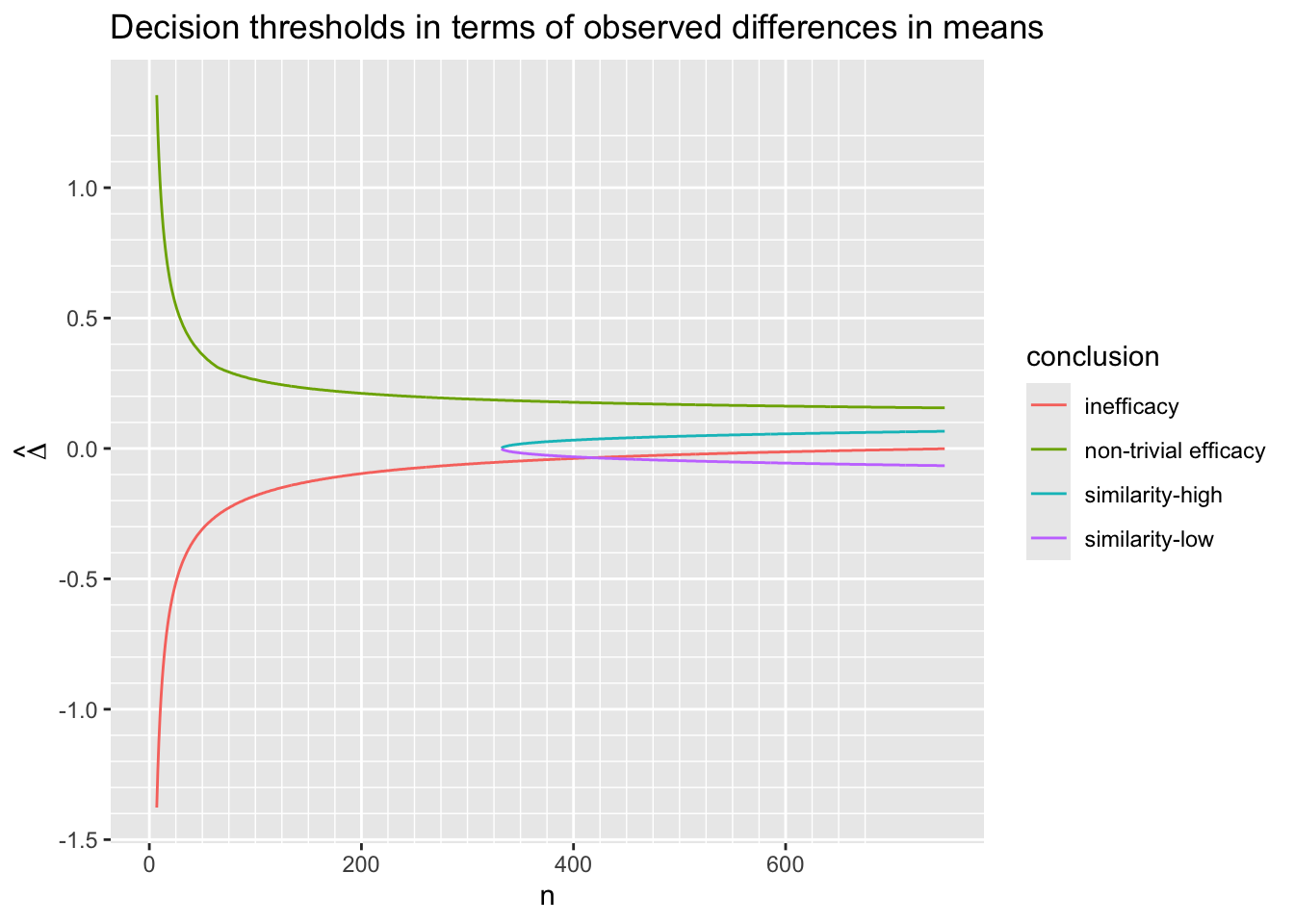
Code
sim.min   <- w[conclusion == 'similarity-low' & ! is.na(Deltahat), min(n)]
sim.max   <- w[conclusion == 'similarity-high' & n == 750, Deltahat]
ineff100  <- w[conclusion == 'inefficacy' & n == 100, Deltahat]
ineff200  <- w[conclusion == 'inefficacy' & n == 200, Deltahat]
nte50     <- w[conclusion == 'non-trivial efficacy' & n == 50, Deltahat]
nte200    <- w[conclusion == 'non-trivial efficacy' & n == 200, Deltahat]
nte.min   <- w[conclusion == 'non-trivial efficacy' & n == 750, Deltahat]
A few observations are in order.
- Similarity can’t be concluded until \(n > 332\)
- Even then the observed difference needs to be almost exactly zero to make that conclusion
- At the maximum sample size \(n=750\) similarity is concluded if the absolute value of the observed \(\hat{\Delta}\) is 0.066 or less (recall that similarity was defined as \(\Delta \in [-0.15, 0.15]\))
- An inefficacy conclusion is possible if \(\hat{\Delta} < -0.181\) when \(n=100\) and if \(\hat{\Delta} < -0.096\) when \(n=200\)
- A non-trivial efficacy conclusion is possible if \(\hat{\Delta} > 0.36\) when \(n=50\) or when \(\hat{\Delta} > 0.211\) when \(n=200\)
- When \(\hat{\Delta} = 0.156\) then planned maximum sample size of \(n=750\) is required to be able to conclude non-trivial efficacy. Recall that the MCID is 0.3 and the threshold for trival effect is \(\Delta=0.1\).
NoteDecision Thresholds on \(z\) Scale
Since the observed treatment effect \(\hat{\Delta}\) has variance \(\frac{2}{n}\) with \(n\) participants per group, the \(\hat{\Delta}\) thresholds are easily converted into the \(z\) scale \(\sqrt{\frac{n}{2}}\hat{\Delta}\).
Code
ggplot(w, aes(x=n, y=Deltahat * sqrt(n / 2), col=conclusion)) + geom_line() +
  scale_x_continuous(minor_breaks=seq(0, 675, by=25)) +
  ylab(expression(z)) +
  labs(title='Decision thresholds on the z-scale')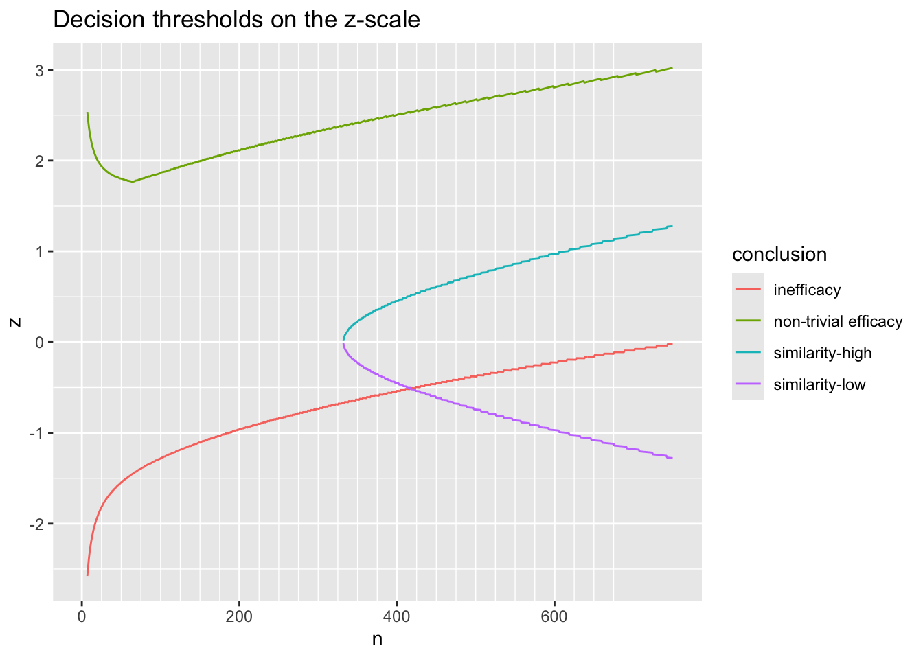
The patterns are different from what is seen with a frequentist approach, as here we see that when \(n > 50\) the critical value for \(z\) increases. That is because we are demanding at least an 0.85 chance that the efficacy is non-trivial (\(\Delta > \gamma\)). The drop in the upper curve from the lowest \(n\) for which a conclusion of non-trivial efficacy is possible (\(n=7\)) to \(n=50\) is due to the influence of the skeptical prior for \(\Delta\) when \(n\) is small. When a flat analysis prior is used for \(\Delta\), the upturn disappears.
9.10.2 Simulation
Now we simulate 10,000 sequential trials for each \(\kappa\) to evaluate the Bayesian operating characteristics. \(\kappa\) and the true unknown treatment effect \(\Delta\) are varied. Studies are allowed to proceed to an upper limit sample size of 750 in each group. Each study is stopped when any stopping criterion is satisfied.
The first function simulates one complete trial, computing the cumulative summary statistic (difference in means) after 1, 2, …, 750 participants in each treatment group.
Code
sim <- function(Delta, kappa, N=750) {
  # Simulate raw data for whole planned trial,
  # for each treatment
  y1 <- rnorm(N,    0., 1.)
  y2 <- rnorm(N, Delta, 1.)
  j  <- 1 : N
  ybar1 <- cumsum(y1) / j
  ybar2 <- cumsum(y2) / j
  Deltahat <- ybar2 - ybar1
  Deltahat  # cumulative mean difference
}
The next function executes the stopping rules for one trial, looking sequentially.
Code
sim1 <- function(Delta, kappa, ignore=59) {
  Deltahat <- sim(Delta, kappa)
  n <- 1 : length(Deltahat)
  # Compute posterior probability of any efficacy
  p1 <- pp(0., Deltahat, n, kappa)
  # Compute probability of non-trivial efficacy
  p2 <- pp(0.10, Deltahat, n, kappa)
  # Compute probability of similarity
  p3 <- pp(-0.15, Deltahat, n, kappa) -
        pp( 0.15, Deltahat, n, kappa)

  # For each decision find first sample size at which criterion was satisfied
  k <- n > ignore
  ineff <- which((p2 < 0.025))[1]   # if which() is empty, empty[1] = NA
  eff   <- which(k & (p1 > 0.95 & p2 > 0.85))[1]
  sim   <- which(k & (p3 > 0.95))[1]
  u <- function(r, n) list(conclusion=r, n=n)
  # If not stopped, trial went to maximum
  All <- c(ineff, eff, sim)
  if(all(is.na(All))) return(u('none', max(n)))
  first <- min(All, na.rm=TRUE)
  if(! is.na(ineff) && ineff == first) return(u('inefficacy', ineff))
  if(! is.na(eff)   && eff   == first) return(u('non-trivial efficacy', eff))
  u('similarity', sim)
}
Run all 50,000 trials. For each \(\Delta\) and \(\kappa\) simulate one clinical trial. Do this over a very fine grid of \(\Delta\) so that we can later smooth the individual results and do not need multiple trials for any one value of \(\Delta\). \(\Delta\)s are drawn from a mean zero normal distribution with \(P(\Delta > 0.75) = 0.025\).
Code
Deltas <- qnorm(seq(0.0001, 0.9999, length=10000), sd=psd(0.75, 0.025))
kappas <- c(0.2, 0.1, 0.05, 0.025, 0.01, 0.001)
set.seed(3)
d <- expand.grid(Delta=Deltas, kappa=kappas)
setDT(d)
d[, .q(conclusion, n) := sim1(Delta, kappa), by=.I]  # 7 sec.
Here are the analysis \(\Delta\) priors. The distribution of the universe of efficacies used to generate the clinical trials has \(\kappa=0.025\).
Code
x <- seq(-2.5, 2.5, length=300)
w <- expand.grid(Delta=x, kappa=kappas)
setDT(w)
w[, sigma := psd(0.75, kappa)]
w[, density := dnorm(Delta, sd=sigma)]
ggplot(w, aes(x=Delta, y=density,
    col=paste0(kappa, ' (', round(sigma, 2), ')'))) + geom_line() +
  xlab(expression(Delta)) + ylab('') +
  guides(color=guide_legend(title=expression(kappa(sigma))))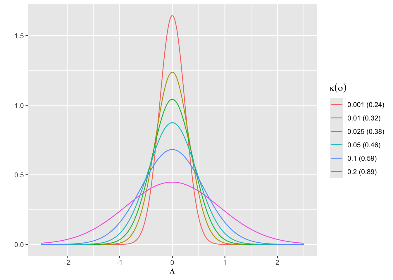
For each \(\kappa\) show the frequencies of stopping for the various conclusions.
Code
w <- d[, table(conclusion, kappa)]
w
kappa
conclusion 0.001 0.01 0.025 0.05 0.1 0.2
inefficacy 4984 5007 5066 5101 5159 5184
non-trivial efficacy 3895 3973 3997 3968 4017 4010
none 242 193 227 194 175 172
similarity 879 827 710 737 649 634Code
R$propconc <- round(prop.table(w, margin=2), 3)The prior skepticism \(\kappa\) has greater impact on stopping for similarity and stopping with no conclusion.
Examine the mean and median stopping time (final N) by reason for stopping and \(\kappa\).
Code
qmean <- function(x) {
  qu <- round(quantile(x, (1:3)/4))
  list(Mean   = round(mean(x)),
       Q1     = qu[1],
       Median = qu[2],
       Q3     = qu[3])
}
w <- d[, qmean(n), by=.(conclusion, kappa)]
options(datatable.print.class=FALSE)
print(w, nrows=100)
conclusion kappa Mean Q1 Median Q3
1: inefficacy 0.200 62 13 31 80
2: non-trivial efficacy 0.200 102 60 60 85
3: similarity 0.200 423 347 378 465
4: none 0.200 750 750 750 750
5: inefficacy 0.100 65 16 35 82
6: non-trivial efficacy 0.100 103 60 60 91
7: similarity 0.100 421 345 381 466
8: none 0.100 750 750 750 750
9: inefficacy 0.050 69 18 38 89
10: non-trivial efficacy 0.050 106 60 60 92
11: similarity 0.050 413 341 367 446
12: none 0.050 750 750 750 750
13: inefficacy 0.025 70 21 41 90
14: similarity 0.025 415 337 368 462
15: non-trivial efficacy 0.025 107 60 60 96
16: none 0.025 750 750 750 750
17: inefficacy 0.010 73 23 44 95
18: similarity 0.010 402 331 357 440
19: non-trivial efficacy 0.010 114 60 60 107
20: none 0.010 750 750 750 750
21: inefficacy 0.001 76 27 49 100
22: similarity 0.001 388 316 338 428
23: non-trivial efficacy 0.001 122 60 64 130
24: none 0.001 750 750 750 750
conclusion kappa Mean Q1 Median Q3Code
R$stopn <- wEven with the most skeptical prior of the four priors, more than half of the simulated studies which ultimately stopped for efficacy could be stopped with that conclusion after just 60 participants, the minimum required for precision. We also need to examine the stopping times counting the other reasons. Here are the mean and median number of participants when stopping is for any reason (including going to the maximum sample size of 750).
Code
w <- d[, qmean(n), by=.(kappa)]
w
kappa Mean Q1 Median Q3
1: 0.200 113 30 60 110
2: 0.100 116 33 60 117
3: 0.050 122 37 60 126
4: 0.025 125 40 60 129
5: 0.010 130 44 60 142
6: 0.001 138 49 65 160Code
R$stopany <- wFor planning purposes the expected sample size may be taken as 138. Sequential analysis without the traditional frequentist limitations on the number of looks makes a large difference in trial efficiency while providing evidence in more dimensions.
Now consider the most important aspect of the performance of the design: the primary Bayesian operating characteristic—correctness of decisions about treatment effect. For our simulation study we judge the alignment between the decision about the treatment effect and the (unknown to us and to the sequential analyses but known to the simulation code) true treatment effect that was in play when the data were simulated. So for each prior and each decision that was made, we estimate the distribution of true treatment effects that were in effect when combining all the simulated trials resulting in that decision. This is the distribution of the \(\Delta\) values conditional on stopping (or going to the sample size limit of 750 for the no-conclusion simulations) and on the reason for stopping. Keep in mind that for the simulations \(\Delta\)s were drawn from \(\kappa=0.025\).
Examine distributions of underlying true \(\Delta\) for each prior and each conclusion (reason for stopping).
Code
del <- c(-0.1, 0, 0.1, 0.3)
ggplot(d, aes(x=Delta, color=conclusion)) + geom_density() +
  facet_wrap(~ kappa, ncol=2) +
  scale_x_continuous(breaks=seq(-1, 1, by=0.5),
                     minor_breaks=seq(-1, 1, by=0.1)) +
  geom_vline(xintercept=del, col='blue', alpha=0.2) +
  xlab(expression(Delta)) + xlim(-1, 1) +
  theme(legend.position='bottom')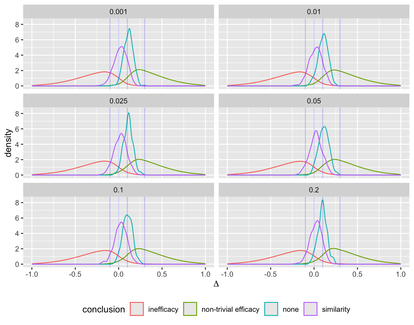
Code
sp <- d[, spikecomp(Delta, tresult='segments'), by=.(conclusion, kappa)]
ggplot(sp) + geom_segment(aes(x=x, y=y1, xend=x, yend=y2, alpha=I(0.3))) +
    scale_y_continuous(breaks=NULL, labels=NULL) + ylab('') +
    facet_grid(conclusion ~ kappa) +
    geom_vline(xintercept=del, col='red', alpha=0.2) +
    xlab(expression(Delta))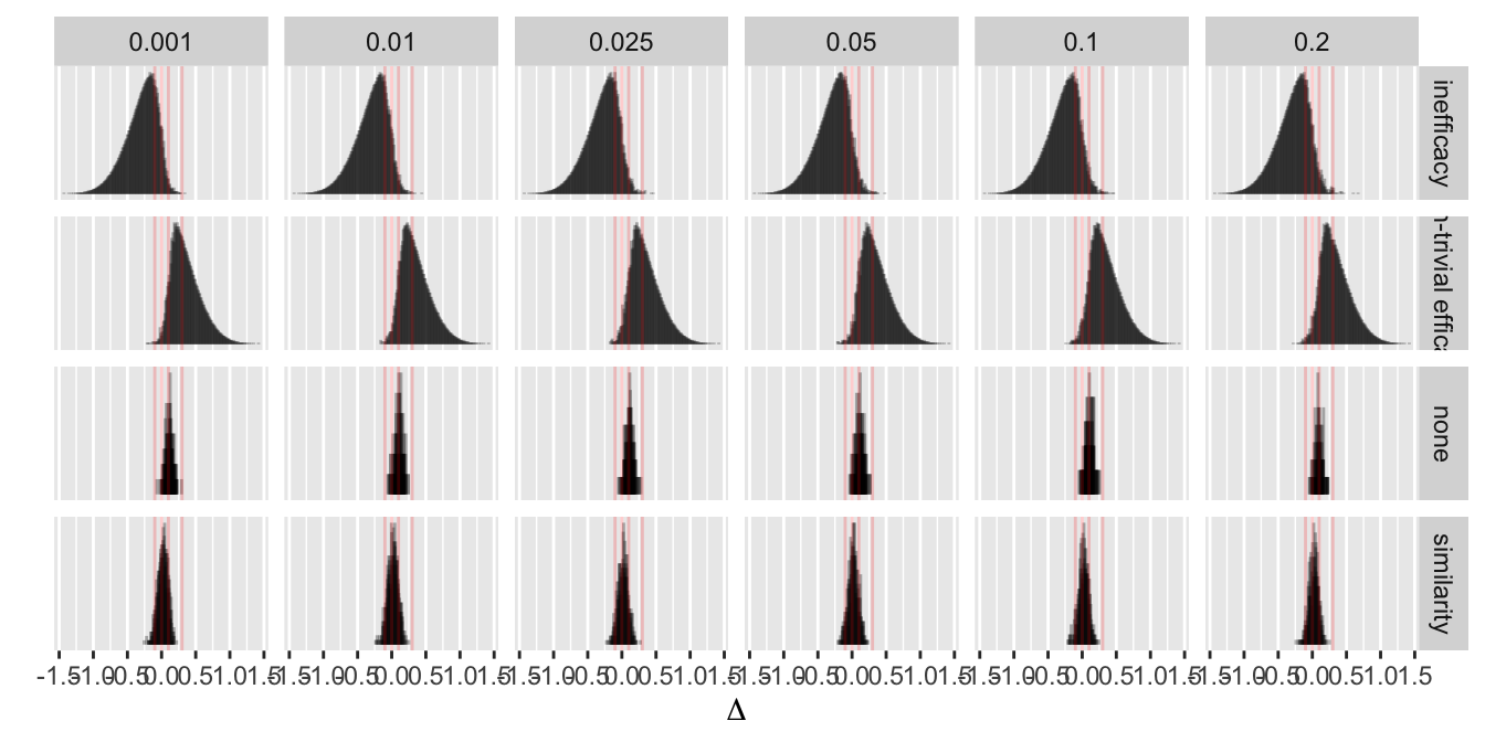
For a conclusion of non-trivial efficacy, the true effect in play was rarely > 0.2. Let’s look at the actual proportions of true \(\Delta\)s in various intervals vs. the conclusion made.
Code
z <- cube(d, .('Δ<0'         = sum(Delta < 0),
              'Δ<0.1'        = sum(Delta < 0.1),
              '-0.15<Δ<0.15' = sum(Delta >= -0.15 & Delta <= 0.15),
              'Δ>0.1'        = sum(Delta > 0.1),
              'Δ>0'          = sum(Delta > 0)),
  by=.q(kappa, conclusion))
z
kappa conclusion Δ<0 Δ<0.1 -0.15<Δ<0.15 Δ>0.1 Δ>0
1: 0.200 inefficacy 4670 5020 1633 164 514
2: 0.200 non-trivial efficacy 97 367 663 3643 3913
3: 0.200 similarity 224 555 607 79 410
4: 0.200 none 9 89 147 83 163
5: 0.100 inefficacy 4659 5012 1622 147 500
6: 0.100 non-trivial efficacy 98 380 677 3637 3919
7: 0.100 similarity 235 554 612 95 414
8: 0.100 none 8 85 139 90 167
9: 0.050 inefficacy 4649 4973 1571 128 452
10: 0.050 non-trivial efficacy 72 351 637 3617 3896
11: 0.050 similarity 273 624 699 113 464
12: 0.050 none 6 83 143 111 188
13: 0.025 inefficacy 4644 4955 1544 111 422
14: 0.025 similarity 270 614 673 96 440
15: 0.025 non-trivial efficacy 81 370 656 3627 3916
16: 0.025 none 5 92 177 135 222
17: 0.010 inefficacy 4609 4915 1504 92 398
18: 0.010 similarity 321 705 784 122 506
19: 0.010 non-trivial efficacy 61 328 612 3645 3912
20: 0.010 none 9 83 150 110 184
21: 0.001 inefficacy 4620 4917 1494 67 364
22: 0.001 similarity 329 747 844 132 550
23: 0.001 non-trivial efficacy 47 270 527 3625 3848
24: 0.001 none 4 97 185 145 238
25: 0.200 <NA> 5000 6031 3050 3969 5000
26: 0.100 <NA> 5000 6031 3050 3969 5000
27: 0.050 <NA> 5000 6031 3050 3969 5000
28: 0.025 <NA> 5000 6031 3050 3969 5000
29: 0.010 <NA> 5000 6031 3050 3969 5000
30: 0.001 <NA> 5000 6031 3050 3969 5000
31: NA inefficacy 27851 29792 9368 709 2650
32: NA non-trivial efficacy 456 2066 3772 21794 23404
33: NA similarity 1652 3799 4219 637 2784
34: NA none 41 529 941 674 1162
35: NA <NA> 30000 36186 18300 23814 30000
kappa conclusion Δ<0 Δ<0.1 -0.15<Δ<0.15 Δ>0.1 Δ>0Code
R$ncorrect <- z
bar <- function(x) round(mean(x), 2)
z <- cube(d, .('Δ<0'         = bar(Delta < 0),
              'Δ<0.1'        = bar(Delta < 0.1),
              '-0.15<Δ<0.15' = bar(Delta >= -0.15 & Delta <= 0.15),
              'Δ>0.1'        = bar(Delta > 0.1),
              'Δ>0'          = bar(Delta > 0)),
  by=.q(kappa, conclusion))
R$correct <- z
g <- function(w, kappa) {
  u <- copy(w)
  if(is.na(kappa)) kappa <- 'All'
  vline <- paste(rep('-', 60), collapse='')
  cat('\n', vline, '\nκ=', kappa, '\n', sep='')
  u[, conclusion := ifelse(is.na(conclusion), 'All', conclusion)]
  print(u)
  invisible()
}
u <- z[, g(.SD, kappa), by=kappa]
------------------------------------------------------------
κ=0.2
             conclusion  Δ<0 Δ<0.1 -0.15<Δ<0.15 Δ>0.1  Δ>0
1:           inefficacy 0.90  0.97         0.32  0.03 0.10
2: non-trivial efficacy 0.02  0.09         0.17  0.91 0.98
3:           similarity 0.35  0.88         0.96  0.12 0.65
4:                 none 0.05  0.52         0.85  0.48 0.95
5:                  All 0.50  0.60         0.30  0.40 0.50

------------------------------------------------------------
κ=0.1
             conclusion  Δ<0 Δ<0.1 -0.15<Δ<0.15 Δ>0.1  Δ>0
1:           inefficacy 0.90  0.97         0.31  0.03 0.10
2: non-trivial efficacy 0.02  0.09         0.17  0.91 0.98
3:           similarity 0.36  0.85         0.94  0.15 0.64
4:                 none 0.05  0.49         0.79  0.51 0.95
5:                  All 0.50  0.60         0.30  0.40 0.50

------------------------------------------------------------
κ=0.05
             conclusion  Δ<0 Δ<0.1 -0.15<Δ<0.15 Δ>0.1  Δ>0
1:           inefficacy 0.91  0.97         0.31  0.03 0.09
2: non-trivial efficacy 0.02  0.09         0.16  0.91 0.98
3:           similarity 0.37  0.85         0.95  0.15 0.63
4:                 none 0.03  0.43         0.74  0.57 0.97
5:                  All 0.50  0.60         0.30  0.40 0.50

------------------------------------------------------------
κ=0.025
             conclusion  Δ<0 Δ<0.1 -0.15<Δ<0.15 Δ>0.1  Δ>0
1:           inefficacy 0.92  0.98         0.30  0.02 0.08
2:           similarity 0.38  0.86         0.95  0.14 0.62
3: non-trivial efficacy 0.02  0.09         0.16  0.91 0.98
4:                 none 0.02  0.41         0.78  0.59 0.98
5:                  All 0.50  0.60         0.30  0.40 0.50

------------------------------------------------------------
κ=0.01
             conclusion  Δ<0 Δ<0.1 -0.15<Δ<0.15 Δ>0.1  Δ>0
1:           inefficacy 0.92  0.98         0.30  0.02 0.08
2:           similarity 0.39  0.85         0.95  0.15 0.61
3: non-trivial efficacy 0.02  0.08         0.15  0.92 0.98
4:                 none 0.05  0.43         0.78  0.57 0.95
5:                  All 0.50  0.60         0.30  0.40 0.50

------------------------------------------------------------
κ=0.001
             conclusion  Δ<0 Δ<0.1 -0.15<Δ<0.15 Δ>0.1  Δ>0
1:           inefficacy 0.93  0.99         0.30  0.01 0.07
2:           similarity 0.37  0.85         0.96  0.15 0.63
3: non-trivial efficacy 0.01  0.07         0.14  0.93 0.99
4:                 none 0.02  0.40         0.76  0.60 0.98
5:                  All 0.50  0.60         0.30  0.40 0.50

------------------------------------------------------------
κ=All
             conclusion  Δ<0 Δ<0.1 -0.15<Δ<0.15 Δ>0.1  Δ>0
1:           inefficacy 0.91  0.98         0.31  0.02 0.09
2: non-trivial efficacy 0.02  0.09         0.16  0.91 0.98
3:           similarity 0.37  0.86         0.95  0.14 0.63
4:                 none 0.03  0.44         0.78  0.56 0.97
5:                  All 0.50  0.60         0.30  0.40 0.50
Code
z <- z[kappa == 0.2]
nte.cor   <- z[conclusion == 'non-trivial efficacy', 6]
nte.any   <- z[conclusion == 'non-trivial efficacy', 7]
ineff.any <- z[conclusion == 'inefficacy', 3]
ineff.cor <- z[conclusion == 'inefficacy', 4]
noconc    <- R$propconc['none', '0.001']
The least favorable result is obtained when \(\kappa=0.2\) when the analysis prior is significantly less skeptical than the way the \(\Delta\)s were generated. To highlight two important points from that first part of the table, for trials that were stopped with a conclusion of non-trivial efficacy, 0.91 of such trials were truly generated by \(\Delta > 0.1\). But 0.98 had any efficacy (\(\Delta > 0\)). For trials stopped for inefficacy, 0.9 of them were generated by a harmful treatment. 0.97 of them were generated by a harmful or at most only trivially effective treatment. Inconclusive studies tended to have treatment effect near \(\Delta = 0.1\). Only about 0.024 of the simulated trials resulted in no conclusion when \(\kappa=0.001\), i.e., wasted resources by randomizing 750 participants to each treatment arm only to have no conclusion at all.
To better understand the “no conclusion” results here are the quartiles and 0.1 and 0.9 quantiles of true \(\Delta\)s in effect when trials went to the maximum sample size without stopping.
Code
g <- function(x) {
  z <- quantile(x, c(10, 25, 50, 75, 90)/100)
  as.list(round(z, 2))
}
d[conclusion == 'none', g(Delta), by=kappa]
kappa 10% 25% 50% 75% 90%
1: 0.200 0.03 0.07 0.10 0.13 0.16
2: 0.100 0.03 0.06 0.10 0.14 0.17
3: 0.050 0.03 0.07 0.11 0.15 0.19
4: 0.025 0.04 0.07 0.11 0.14 0.17
5: 0.010 0.03 0.07 0.11 0.14 0.18
6: 0.001 0.04 0.07 0.12 0.15 0.18The median true \(\Delta\) when no conclusion could be reached was very near \(\gamma = 0.1\), the threshold for triviality of treatment effect. So \(\frac{1}{2}\) of the futile trials were generated by trivial efficacy. Very few if any of the trials were generated by a completely ineffective treatment (\(\Delta < 0\)).
Finally, examine the distribution of true \(\Delta\) values as a function of deciles of stopping time, when the conclusion was non-trivial efficacy.
Code
sp <- d[conclusion=='non-trivial efficacy',
        spikecomp(Delta, tresult='segments'), by=cut2(n, g=10)]
ggplot(sp) + geom_segment(aes(x=x, y=y1, xend=x, yend=y2, alpha=I(0.3))) +
    scale_y_continuous(breaks=NULL, labels=NULL) + ylab('') +
    facet_wrap(~ cut2) +
    geom_vline(xintercept=del, col='red', alpha=0.2) +
    xlab(expression(Delta))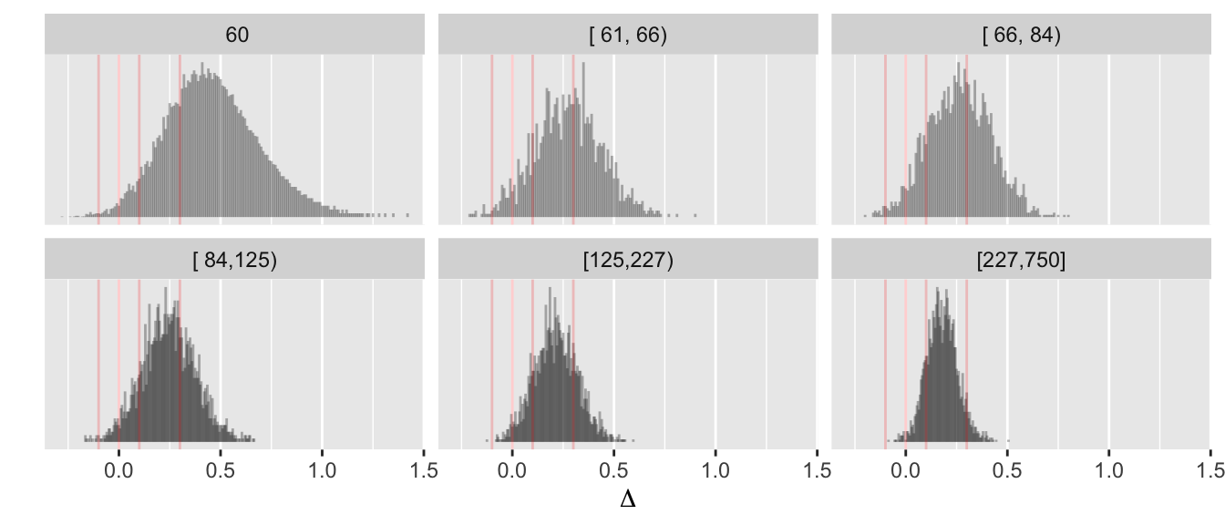
Many studies stopped at the minimum of N=60 and these were reliable in judging the treatment to have more than trivial efficacy.
9.10.3 Bayesian Operating Characteristics of Frequentist Procedure
Consider the expected sample size and Bayesian operating characteristics (probability that made decisions are correct) of a frequentist group sequential testing procedure. The R gsDesign package is used to compute the group sequential one-sided stopping boundaries. The following changes are made from what was done for the simulation of the Bayesian procedure:
- use a one-sided test and one-sided stopping boundaries to give the frequentist procedure the benefit of the doubt when comparing with a directional Bayesian decision rule
- This results in a smaller sample size for a single-look fixed \(N\) design
gsDesignonly allows 30 data looks for O’Brien-Fleming boundaries; for the less conservative Hwang-Shih-DeCani (HSD) boundaries (the default ingsDesign), continuous looks are still not possible, but the stopping boundary algorithm works for looks after every 5 patients are accrued when the first look is at \(N=60\). The following simulation will use the HSD algorithm with \(\gamma=-4\) looks at \(N=60, 65, 70, ..., 750\) for efficacy and similarity, but will start looking at \(N=5\) for inefficacy. These HSD bounds are among the least conservative bounds that still use a close-to-nominal \(\alpha\) at the final look.- The minimum precision sample size of \(N=60\) is respected for efficacy and similarity, and three stopping rules are implemented, in this order: stopping for evidence of inefficacy/trivial efficacy, for non-trivial efficacy, and for similarity. Note that the minimum sample size of 60 per group for assessing similarity is not really consequential, as conclusions of similarity require much larger sample sizes than that.
For this \(N=60, 65, ..., 750\) scheme, there is an anomaly with HSD boundaries—they are not monotonic in \(N\), taking a turn at around \(N=90\). Per Keaven Anderson, author of
gsDesign, the bound is smaller on the left due to waiting until the initial sample is \(N=60\) before doing the first analysis, and then incrementing by small amounts of \(\alpha\) thereafter.Compute the sample size needed for a fixed design with one-sided \(\alpha=0.05\) and power of 0.9. The one-sided frequentist power for a one-tailed test with \(\alpha=0.05\) is \(1 - \Phi(1.645 - \frac{0.3}{\sqrt{\frac{2}{n}}})\), and setting this to 0.9 requires \(n=2[\frac{1.645 + 1.282}{0.3}]^2 = 190\).
Compute HSD one-sided stopping boundaries for efficacy assessment at \(N=60, 65, ..., 750\) and inefficacy assessment at \(N=5, 10, 15, ..., 750\). Recall that \(N\) is per group. The inefficacy stopping boundaries would be identical to the efficacy boundaries had they had the same look schedule. This is because the one-sided test for inefficacy merely shifts the observed mean difference by the triviality threshold \(\gamma\). The inefficacy boundary is actually the negative of what is plotted below.
Code
require(gsDesign)
eff_looks   <- seq(60, 750, by=5)
ineff_looks <- seq( 5, 750, by=5)
gs          <- gsDesign(k = length(eff_looks), test.type = 1, alpha = 0.05, timing = eff_looks / 750)
upper_eff   <- gs$upper$bound
gs          <- gsDesign(k = length(ineff_looks), test.type=1, alpha=0.05, timing = ineff_looks / 750)
lower_ineff <- - gs$upper$bound
gs          <- gsDesign(k = length(eff_looks), test.type=1, alpha = 0.025, timing = eff_looks / 750)
upper_sim   <- gs$upper$bound
d <- rbind(data.frame(type = 'efficacy',   n = eff_looks,   bound =   upper_eff),
           data.frame(type = 'inefficacy', n = ineff_looks, bound = - lower_ineff),
           data.frame(type = 'similarity', n = eff_looks,   bound =   upper_sim))
ggplot(d, aes(x=n, y=bound, color=type)) + geom_line() + xlab('N') + ylab('Boundary')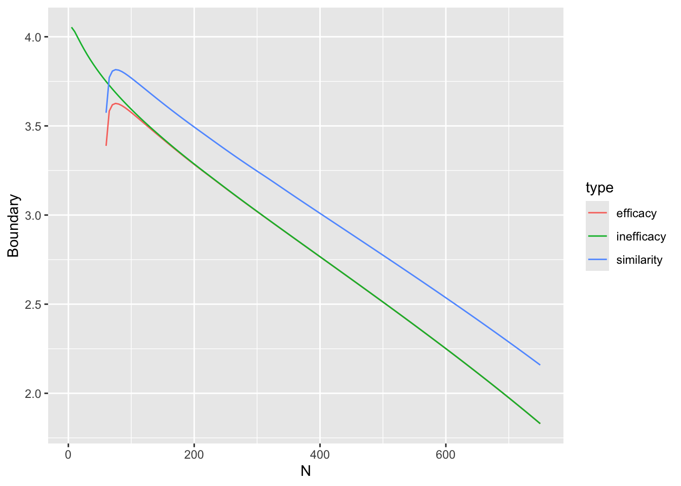
Find the stopping boundary for efficacy at \(N = 190\).
Code
crit <- upper_eff[eff_looks == freqN1]
crit
[1] 3.311607Let’s see how much power is lost from multiplicity adjustment when the look is at $N=190. The power is \(1 - \Phi(3.3116067 - \frac{0.3}{\sqrt{\frac{2}{190}}})\)
Code
pow <- pnorm(crit - 0.3 / sqrt(2 / freqN1))
pow
[1] 0.6508323The multiplicity-adjusted power is so much lower than 0.9 because the group sequential-adjusted critical value of 3.3116067 is so much larger than 1.645. The power at the highest planned sample size of 750 would be barely affected by the sequential frequentist multiplicity adjustment, but \(N=750\) is a long time to wait for results.
Alternate procedures such as sample size restimation do not solve this problem because they require discounting of early results when combining early with extended data, to preserve \(\alpha\).
For assessing evidence for similarity, use the standard conservative TOST procedure – two one-sided tests. To correspond to a Bayesian interval with 0.95 probability as we are using, TOST must use \(\alpha=0.025\). To conclude similarity with similarity bounds of \([-0.15, 0.15]\) at the overall upper bound of \(\alpha=0.025\) we must reject both \(H_{0}: \Delta \leq -0.15\) and \(H_{0}: \Delta \geq 0.15\) at the \(\alpha=0.025\) level. To make this a group sequential test we use the group sequential stopping boundaries rather than the (smaller) standard normal critical values.
Similarity assessment uses the same look schedule as efficacy so has the same group sequential stopping boundaries as efficacy, since each of the two one-sided tests is at one-sided \(\alpha=0.05\).
Let’s implement the triple stopping rules: stopping early for inefficacy (less than trivial efficacy), non-trivial efficacy, or similarity. The value of \(\kappa\) chosen to describe the universe of zero-mean treatment effects used in the simulation is 0.025, i.e., \(P(\Delta > 0.75) = 0.025\).
Simulate one complete trial, computing the cumulative summary statistic (difference in means) after 1, 2, 3, …, 750 participants are in each treatment group.
Code
sim <- function(Delta, N=750) {
  # Simulate raw data for whole planned trial,
  # for each treatment
  y1 <- rnorm(N,    0., 1.)
  y2 <- rnorm(N, Delta, 1.)
  j  <- 1 : N
  ybar1 <- cumsum(y1) / j
  ybar2 <- cumsum(y2) / j
  Deltahat <- ybar2 - ybar1
  Deltahat  # cumulative mean difference at all possible looks
}
Define a function that executes the frequentist stopping rules for one trial, looking sequentially at sample sizes in eff_looks and ineff_looks (efficacy and inefficacy looks).
Code
mn <- function(a, b) if(any(b)) min(a[b]) else NA
sim1 <- function(Delta) {
  Deltahat <- sim(Delta)
  # Compute z statistic for any efficacy
  z1  <- Deltahat[eff_looks] / sqrt(2 / eff_looks)
  # Compute z statistic for inefficacy (trivial or no or negative efficacy)
  z2  <- (Deltahat[ineff_looks] - 0.1) / sqrt(2 / ineff_looks)
  # Compute z statistic for one-sided tests uses in TOST for similarity
  z3L <- (Deltahat[eff_looks] + 0.15) / sqrt(2 / eff_looks)
  z3U <- (Deltahat[eff_looks] - 0.15) / sqrt(2 / eff_looks)

  # For each decision find first sample size at which criterion was satisfied
  ineff <- mn(ineff_looks, z2  < lower_ineff)
  eff   <- mn(eff_looks,   z1  > upper_eff)
  simi  <- mn(eff_looks,   z3L > upper_sim & z3U < - upper_sim)

  u <- function(r, n) list(conclusion=r, n=n)
  # If not stopped, trial went to maximum
  if(is.na(ineff) && is.na(eff) && is.na(simi)) return(u('none', max(eff_looks)))
  first <- min(ineff, eff, simi, na.rm=TRUE)
  if(! is.na(ineff) && ineff == first) return(u('inefficacy',           ineff))
  if(! is.na(eff)   && eff   == first) return(u('non-trivial efficacy', eff))
  if(! is.na(simi)  && simi  == first) return(u('similarity',           simi))
  stop('program logic error')
}
Run all 10,000 trials. For each \(\Delta\) simulate one clinical trial.
Code
Deltas <- qnorm(seq(0.0001, 0.9999, length=10000), sd=psd(0.75, 0.025))
set.seed(5)
d <- data.table(Delta=Deltas)
d[, .q(conclusion, N) := sim1(Delta), by=.I]  # 0.5 sec.
cat('\nNumber of trials reaching each conclusion:\n\n')
Number of trials reaching each conclusion:Code
freqconc <- d[, .N, by=conclusion]
freqconc
conclusion N
1: inefficacy 4868
2: similarity 589
3: none 432
4: non-trivial efficacy 4111Code
R$freqconc <- freqconcEstimate typical stopping times as a function of \(\Delta\) for each conclusion.
Code
ggplot(d, aes(Delta, N, col=conclusion)) + geom_smooth(method=loess) +
  xlab(expression(Delta)) + ylab('Average N Per Group')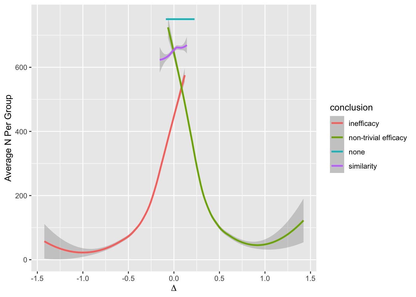
Examine the mean and median stopping time (final N per group) by reason for stopping.
Code
w <- cube(d, qmean(N), by=.q(conclusion))
w
conclusion Mean Q1 Median Q3
1: inefficacy 202 75 150 290
2: similarity 652 610 640 690
3: none 750 750 750 750
4: non-trivial efficacy 254 90 190 375
5: <NA> 273 90 195 415Code
R$stopn_freq <- wLet’s look at the actual proportions of true \(\Delta\)s in various intervals vs. the conclusion made.
Code
z <- cube(d, .('Δ<0'         = sum(Delta < 0),
              'Δ<0.1'        = sum(Delta < 0.1),
              'Δ>0.1'        = sum(Delta > 0.1),
              'Δ>0'          = sum(Delta > 0),
              '-0.15<Δ<0.15' = sum(Delta >= -0.15 & Delta <= 0.15)),
          by=.q(conclusion))
z
conclusion Δ<0 Δ<0.1 Δ>0.1 Δ>0 -0.15<Δ<0.15
1: inefficacy 4699 4866 2 169 1395
2: similarity 253 558 31 336 587
3: none 38 316 116 394 407
4: non-trivial efficacy 10 291 3820 4101 661
5: <NA> 5000 6031 3969 5000 3050Code
R$ncorrect_freq <- z
z <- cube(d, .('Δ<0'         = bar(Delta < 0),
              'Δ<0.1'        = bar(Delta < 0.1),
              'Δ>0.1'        = bar(Delta > 0.1),
              'Δ>0'          = bar(Delta > 0),
              '-0.15<Δ<0.15' = bar(Delta >= -0.15 & Delta <= 0.15)),
  by=.q(conclusion))
z
conclusion Δ<0 Δ<0.1 Δ>0.1 Δ>0 -0.15<Δ<0.15
1: inefficacy 0.97 1.00 0.00 0.03 0.29
2: similarity 0.43 0.95 0.05 0.57 1.00
3: none 0.09 0.73 0.27 0.91 0.94
4: non-trivial efficacy 0.00 0.07 0.93 1.00 0.16
5: <NA> 0.50 0.60 0.40 0.50 0.30Code
R$correct_freq <- z
if(FALSE) {   ## ???
g <- function(w, kappa) {
  u <- copy(w)
  if(is.na(kappa)) kappa <- 'All'
  vline <- paste(rep('-', 60), collapse='')
  cat('\n', vline, '\nκ=', kappa, '\n', sep='')
  u[, conclusion := ifelse(is.na(conclusion), 'All', conclusion)]
  print(u)
  invisible()
}
u <- z[, g(.SD, kappa), by=kappa]
z <- z[kappa == 0.2]
nte.cor   <- z[conclusion == 'non-trivial efficacy', 6]
nte.any   <- z[conclusion == 'non-trivial efficacy', 7]
ineff.any <- z[conclusion == 'inefficacy', 3]
ineff.cor <- z[conclusion == 'inefficacy', 4]
noconc    <- R$propconc['none', '0.001']
}
In the chart below, frequentist group sequential procedure performance appears in parentheses.
The frequentist sequential procedure is seen as ultra-conservative by a Bayesian. Because of its conservatism, when a group sequential stopping rule triggers, the conclusion has a high probability of being correct. The problem is that the frequentist design draws conclusions far too late. Expected sample sizes are more than double that required for the simple Bayesian sequential design, which benefits greatly from having no multiplicities to penalize for.
Group sequential designs are touted as providing a safety net for patients enrolled in clinical trials, by looking for early harm from a treatment. This is misleading because the power of group sequential methods is extremely low at early looks. This would be even more of a problem were O’Brien - Fleming stopping boundaries used instead of HSD used here.
9.11 Borrowing Information
- When the treatment has been well studied in prior randomized clinical trials it is reasonable to use at least some of that information in the prior distribution for the treatment effect in the new study
- Some discounting is required because there may be doubt about
- similarity of patients
- general time trends in outcomes
- changes in concomitant therapies that could detract from efficacy estimated in patients before such therapies were in use
- changes in how outcomes are measured including duration of follow-up
- Some ideal situations for borrowing of information include
- use of a device on a bone that is not the bone previously studied, or use on skin on another part of the body from that studied
- studying a device that is a tweak of a device that has been extensively studied previously
- use of a drug on a different patient population where the difference in patients is not directly related to what the drug is intended to prevent
- use of adult data about a drug to inform efficacy for treating the same disease in children
- use of a device on a bone that is not the bone previously studied, or use on skin on another part of the body from that studied
- The posterior probability distribution of the treatment effect from the earlier study/studies becomes part of the prior
- Important to include results from randomized studies that showed unimpressive treatment effects along with those that were “positive”; no cherry picking allowed
- Discounting can be done a variety of ways, including power priors and mixtures of priors
- Mixtures of priors are appealing and more interpretable
- Mix a prior \(f_1\) that is somewhat skeptical of large treatment effects from the new data alone with an optimistic prior \(f_2\) from previous studies
- Prior for the new study: \(f(\theta) = (1 - a) f_{1}(\theta) + a f_{2}(\theta)\)
- \(a\) may be directly interpreted as the applicability of the previous data to the current comparison
- Applicability can be thought of in two ways (see below); for purpose of Bayesian analysis which of the two you prefer does not matter
- For either notion of applicability, uncertainties (width of posterior distribution from previous studies) must be carried forward
- Applicability is a number between 0 and 1 and is either
- The degree to which you think that relative efficacy of treatment as learned from previous trials applies as the relative efficacy in the current trial or
- The probability that what is learned about relative efficacy in previous studies fully applies to the new study
- To anchor the values:
- \(a=0 \rightarrow\) previous data should be completely ignored
- \(a=1 \rightarrow\) previous data are completely relevant and the new study is unnecessary
- To justify a value of \(a\) one should undertake a survey on a reasonable number (say 12-20) of experts including, for drug studies, clinical pharmacologists familiar with absorption and metabolism of the drug in different patient types
- See this for excellent work the FDA has done related to borrowing adult data for pediatric drug trials
But it is important to note that strong arguments can be made for including the raw data from other studies in a joint analysis with the new trial data, instead of summarizing the other data through a posterior distribution that is converted to a prior and then down-weighted. Down-weighting can come from adding a bias parameter for the historical data when forming the joint new data/old data Bayesian models. Major advantages of this approach include
- using a standard simple prior (e.g., Gaussian) for discounting
- making assumptions more explicit
- explicitly modeling bias
- getting more accurate analysis, for example by not assuming normality for a point estimate from historical data
- covariate adjustment
This last point is all-important. If there is a shift in the distribution of important prognostic factors between two data sources, this shift can be handled elegantly and simply using standard covariate adjustment. This is far more effective and efficient than matching or playing with inclusion criteria. Without analyzing the raw data, the effect of covariate shifts is very hard to counter, especially when the outcome model is nonlinear. It is often unclear what part of the covariate distribution (e.g., shift in means vs. a shift in only one of the tails) should be accounted for when using summary and not raw data.
A simple case study in joint raw data modeling for incorporating historical control data into an RCT may be found at fharrell.com/post/hxcontrol. The joint analysis is facilitated by the Bayesian approach, which allows one to specify any number of models for joint analysis. When the models share one or more parameters, interesting things happen. The case study illustrates that
- When the new RCT has some but not enough control patients, and control information from historical data is incorporated into the analysis, the prior distribution for the bias in the historical data is important. The amount of bias can be estimated.
- When the new RCT has no controls, so that control information is coming only from the historical data, the prior distribution for the bias in the historical data is incredibly important. The amount of bias cannot be estimated from the data at hand, and comes solely from the bias parameter’s prior distribution. This truly reflects the limitation of not having concurrent controls.
9.11.1 Example Joint Data Model
- RCT control: \(Y \sim n(\mu_{c}, \sigma)\)
- RCT active: \(Y \sim n(\mu_{a}, \sigma)\)
- Historical control: \(Y \sim n(\mu_{c} + b, \sigma)\)
- Bias \(b \sim n(0, \tau)\)
- \(\tau\) controls amount of borrowing
- \(\tau = \infty\): historical data irrelevant
- \(\tau = 0\): historical data trusted as much as within-study control data
- Historical data and concurrent controls are estimating the same thing
9.11.2 Extension to Extrapolation
- Let \(X\) be the extrapolation factor (e.g., age)
- At the root is treatment \(\times X\) interaction
- Model: \(Y \sim n(\beta_{0} + \beta_{1}Tx + \beta_{2}X + \beta_{3}\text{Tx} \times X, \sigma)\)
- No restriction on \(\beta_{3} \rightarrow\) new study stands on its own
- Skeptical prior on \(\beta_{3} \rightarrow\) borrow information
- Can also add a nonlinear interaction with a more skeptical prior
fharrell.com/post/ia quantifies how non-overlap of \(X\) distributions relates to the precision of \(X\)-specific treatment effects.