1 High-Level View
Evidence-building for therapeutic effectiveness can be based solely on Bayesian ideas. This allows maximum design flexibility while maintaining rigor, and simplifies analyses and their interpretation. Bayesian design and analysis strategies can be based on
- prior distributions for the unknown treatment effect that are chosen collaboratively
- priors that merely place constraints on treatment effects (e.g., low probability of extensive benefit or extensive harm) in the usual case where there is no solid existing evidence, but the treatment is known to be incremental rather than curative
- purely Bayesian operating characteristics such as the chance that the trial will result in definitive evidence (e.g., posterior probability \(> 0.95\)) for efficacy, similarity, non-inferiority, inferiority, or futility
- choosing maximum sample size and interim analysis schedule based on those operating characteristics, and estimating a distribution for the actual sample size
- executing the design, which can allow for complex adaptations with no increase in analysis complexity
- summarizing evidence with the last-computed posterior probability that efficacy \(> E\) for any desired value of \(E\) (or posterior probability of non-inferiority, etc.)
Frequentist operating characteristics are not needed in the Bayesian paradigm, and Bayesian operating characteristics are more direct and easier to simulate, e.g., simulate 10,000 trials over a continuous distribution of unknown efficacy \(E\) and estimate, as a function of \(E\), the probability of ever hitting a posterior probability \(> 0.95\) over the planned sequential data looks (including the final planned look).
Error probabilities in the Bayesian setting “come along for the ride” and pertain to actual decision errors and not \(\alpha\). If one acts as if the treatment works after computing a Bayesian posterior probability of efficacy of 0.96, the probability that the wrong action was taken is 0.04.
Would a regulator rather know
- the chance of making an assertion of efficacy if a drug has no effect
or - the chance that the drug is ineffective (either has no effect or harms the patient)?
Bayesian modeling provides the perfect point in the logic flow at which to inject context-specific skepticism, or relevant positive evidence from other studies
So the Bayesian and frequentist approaches are based on inverse measures: one deals with probabilities of hypotheses given the data and the other involves probabilities of data sets given hypotheses. — Berry (1987)
A fundamental tenet of the Bayesian approach: data does not create beliefs; rather it modifies existing beliefs.
We need an evidence measure that ignores ignorable contexts and factors in contexts that matter. And instead of computing a measure of data surprise if the null hypothesis is true, Bayes reacts to whatever unknown value of the parameter is thrown at it, focused by the prior.
What is the principal distinction between Bayesian and classical statistics? It is that Bayesian statistics is fundamentally boring. There is so little to do: just specify the model and the prior, and turn the Bayesian handle. There is no room for clever tricks or an alphabetic cornucopia of definitions and optimality criteria. — Dawid (2000)
With Bayes you start with a prior distribution for θ and given your data make an inference about the θ-driven process generating your data (whatever that process happened to be), to quantify evidence for every possible value of θ. With frequentism, you make assumptions about the process that generated your data and infinitely many replications of them, and try to build evidence for what θ is not.
1.1 Essence of Bayes
Bayesian statistics is a mechanism for rationally updating beliefs in the light of new data. It is tailored for decision making. Here are some of its features.
P-values assume no drug effect and compute the probability of observing data more extreme than yours; the Bayesian posterior probability is the chance the effect is positive given the observed data.
The second is the type I error. An example of the first is the chance of a positive drug effect of 0.98, which means that one has a 0.02 chance of being wrong, whether or not the drug is approved. A type I (long-run false positive chance) error of 0.05 may be useful when designing the study, but once results are available p=0.03 is just a measure of how surprising the data are if the null hypothesis is true, and gives no clue about our evidence for the null and only indirect evidence for the non-null.
The chance that blood pressure is lowered \(\geq\) 5mmHg, the chance that at least 3 of 5 efficacy endpoints are improved by the drug.
The current chance the drug is effective has the same intrepretation whether or not this probability was also computed 100 subjects ago.
Frequentist methods must envision replications of the experiment and must incorporate the intended analysis schedule in computing probabilities of data extremes under the null, which can be very complicated. Forward Bayesian posterior probabilities are merely functions of the prior distribution and the current data and are computed the same whether in the context of a simple one-look data analysis or in an analysis conducted inside a complex adaptive or sequential strategy.
It is easy to compute the chance of a positive drug effect on two clinical endpoints in children at the 10th data look given a specific skeptical prior distribution for this effect, the posterior distribution from an adult trial, and given that the adult data are 0.7 relevant to children.
1.2 Statistical Big Picture
- Traditional frequentist approach: try to gather evidence against the null
- To obtain indirect evidence for a drug effect, show that assuming the null leads to an unlikely observation
- Type I assertion probability \(\alpha\): Prob(asserting efficacy when drug effect is exactly 0); does not use data
- Is not the probability of making an error (that would be Prob(drug doesn’t work if we conclude it does))
- p-value: Prob(someone else’s data more impressive than mine if exact study design could be repeated and the null were exactly true)
- p-value does not tell us the degree to which observed efficacy was due to random chance (that would be Prob(H0) whereas a p-value assumes H0)
What is needed for decision making?
- A forecast of what will happen
- how likely it is that the drug works
- predicting what we don’t know
- Utility/loss/cost function - consequences of
- acting as if an event will happen (or drug is effective)
- acting as if the event won’t happen (or the drug is ineffective)
- Make decision to optimize expected utility
- for all possible magnitudes of efficacy (E), integrates
- likelihood of efficacy being E (degree of belief) and
- utility of making a pro-efficacy decision if it were E
- for all possible magnitudes of efficacy (E), integrates
- Example: betting on a game involves your estimate of the chance a team will win, not the value of a past state should the team ultimately win
- Decision making is in forward-mode; doesn’t assume a truth and work backwards
What about uncertainty, data, evidence, and beliefs?
- Probability is our best way of of capturing uncertainty about unknowns
- Probability is always subjective, depending on the information available to the beholder
- Outside of long-run relative frequencies in simple examples, we require statements about one-time events
- E.g.: whatever produced our data, what’s the chance that positive efficacy was behind it?
- Frequentist: what should I do?; Bayesian: what should I believe and to what degree? (Blume (2002))
- automated dichotomous decisons are always arbitrary (e.g., p-value cutoffs) and oversimplified (ignore clinical significance)
- Bayes provides an objective way for building beliefs
- To get beliefs out, you must put beliefs in
- one cannot compute a posterior (post-data) probability without an anchor (prior probability)
1.3 Drug Approval
- Based on totality of evidence for efficacy & safety
- Approvals seldom revisited unless safety problems emerge
- Benefit-risk tradeoff: need to demonstrate more efficacy when there is a (nonfatal) safety signal
Types of errors in regulatory process:
- Disapproval for a drug that is actually safe and effective
- Approval of a drug that is safe but whose effectiveness has been overestimated and is positive but clinically trivial
- Approval of a drug that is not effective but is safe
- Approval of a drug that is not effective and not safe
- Approval of a drug that has negative effectiveness but is safe (e.g. drug slightly raises blood pressure)
- Approval of a drug that has negative effectiveness and is unsafe
| Statistical evidence that drug works | ||
|---|---|---|
| + | - | |
| Drug works | correct | incorrect |
| Drug doesn’t work | incorrect | correct |
- False positive: lower left entry; Prob(false +) = Prob(drug doesn’t work | statistical evidence it works)
- A Bayesian quantity; not available with frequentist paradigm
- Frequentist Prob(statistical evidence + | drug has zero effect)
- This is not Prob(regulator’s regret)
- Just as with specificity of a diagnostic test, is not very relevant once the data (test) are known
There are members of regulatory authorities who have claimed that one of their roles is to have a successful track record in terms of there being a low proportion of approved drugs that turn out to be ineffective. However, regulatory authorities are not charged with evaluating a new treatment in the context of other sponsors, RCTs, and treatments when this contextualization involves discounting the evidence at hand from a single RCT. But even if this fell under regulatory perview, it is just not possible to estimate long-run performance under the frequentist paradigm.
A true error probability: The chance that a treatment is truly ineffective when there is a specific evidence for efficacy, quantified with a posterior probability.
To better understand the vast difference between Bayesian thinking and traditional frequentist thinking, consider long-run performance of a Bayesian decision process based on statistical evidence over a series of RCTs. Consider one decision direction—acting as if a treatment works, i.e., has efficacy in the right direction. How would one estimate the expected number of approved treatments that were actually ineffective or harmful? Suppose that in 4 RCTs the Bayesian posterior probabilities of positive efficacy were 0.9, 0.96, 0.99, and 0.94 and that one has agreed to use certain (but possibly different) prior distributions for each of the studies. The expected number of RCTs for which efficacy was truly in the right direction is 0.9 + 0.96 + 0.99 + 0.94 = 3.79. The expected number of mistakes among these 4 approvals is 4 - 3.79 = 0.21. This is what long-run statistical performance looks like, if it were to be of interest, and it is not possible to estimate these expected numbers using frequentist statistics.
Now turn to the usual situation where evidence is assessed primarily from a study at hand. The error probability that matters the most is the probability of being wrong in acting as if the treatment performs in a given way. For the moment suppose the evidence favors efficacy and the error probability of interest is the probability of being wrong in acting as if the treatment works. Let
- \(a\) denote the agreed-upon prior distribution selected during study design, called the analysis prior
- \(s\) denote a prior distribution that may be in effect for an empowered critic of the study design, called the sampling prior or simulation prior
Let’s suppose that substantial evidence entails a probability exceeding 0.95 that the treatment effect is in the right direction under \(a\). Then the error probability of interest is the probability that efficacy is zero or in the wrong direction when the posterior probability of it being in the right direction is, say 0.96, calculated under \(a\). To an observer who uses \(a\) the probability of the substantial evidence being misleading is by definition 0.04. In general if we let \(\Delta\) be the true unknown treatment difference, with positive \(\Delta\) denoting benefit, the probability of being wrong in the efficacy assessment, i.e., the probability that the substantial evidence for efficacy is misleading, is \(P(\Delta \leq 0 | P(\Delta > 0 | \mathrm{data}, a) = 0.96, s)\) = 0.04 when \(s = a\).
So for a Bayesian assessment of evidence for efficacy when one is currently focusing on evidence for positive efficacy there are two major tasks of interest:
- determining at the design stage who are the “observers who matter” and incorporating their prior into the agreed upon single prior \(a\) (which is a skeptical prior when no information is being borrowed from other studies), or
- computing \(P(\Delta < 0 | P(\Delta > 0 | \mathrm{data}, a) = p), a), s \neq a)\) to determine if its meaningfully far from \(P(\Delta \leq 0 | P(\Delta > 0 | \mathrm{data}, a) = 0.96, s=a)\).
See here for example calculations of the probabilities of making a mistake from the standpoints of the study designers and a critic whose prior disagrees with the designer’s.
See Also
- When the Alpha is the Omega: P-values, “Substantial Evidence,” and the 0.05 Standard at FDA by Lee Kennedy-Shaffer
1.4 Statistical Inference
- 3 statistical paradigms: frequentist, likelihood, Bayesian
- Bayesian: more clear/clinically relevant interpretation, solve complex problems e.g. inference in sequential/adaptive designs
- Also provides:
- a way to incorporate extra-study information
- quantification of evidence for clinical significance
- draw simultaneous inference about multiple endpoints
- easy simple-size re-estimation
- exact inference under non-normality
- Frequentist approach objective at the beginning
- but endless subjective debates at the end (how to translate evidence about data to evidence about effects, multiplicity, benefit:risk, totality of evidence)
- Bayesian approach involves subjectivity in quantifying beliefs at beginning
- but at the end results in concise clinically relevant statements about beliefs, updated by data
- pre-specification of how all final evidential quantities are to be computed
See Also
frequentist, likelihood, and Bayesian paradigms overview by S Senn
introduction and reading list by Etz, et al.
Heuts et al. (2024), Ionan et al. (2023), Ruberg et al. (2023), Bendtsen (2018), Kruschke (2013), Kruschke & Liddell (2017), Kruschke (2015), Berry (2006), Spiegelhalter et al. (2004), Albert (2007), McElreath (2016), Lindley (1993)
An excellent paper (Lindley (1993)) may be found here
This paper gives a clear explanation of the fundamental problem with p-values and why it is necessary to bring background information into the analysis.The case for a Bayesian approach to benefit-risk assessment by Costa et al.
Richard McElreath’s online lectures
Mark Lai’s Course handouts for Bayesian Data Analysis
Ionan et al. (2022): usage of Bayesian methods at FDA CDER and CBER
Natanegara et al. (2014): survey of pharmaceutical industry, regulatory, and research institutions to determine hindrances to adoption of Bayesian approaches in medical product development:
insufficient knowledge about the Bayesian approach
lack of clarity from regulatory authorities
need for better Bayesian training
need for fully worked-out case studies
need for more information about trial design, sample size determination, success criteria, and interim decisions
1.5 Comparison of Frequentist and Bayesian Approaches
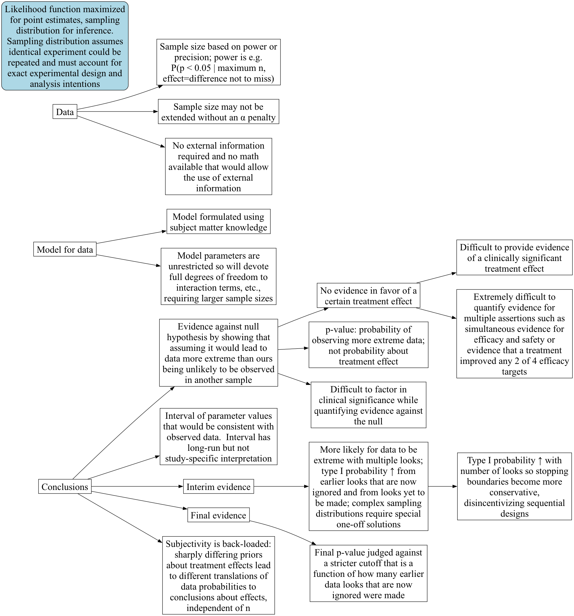
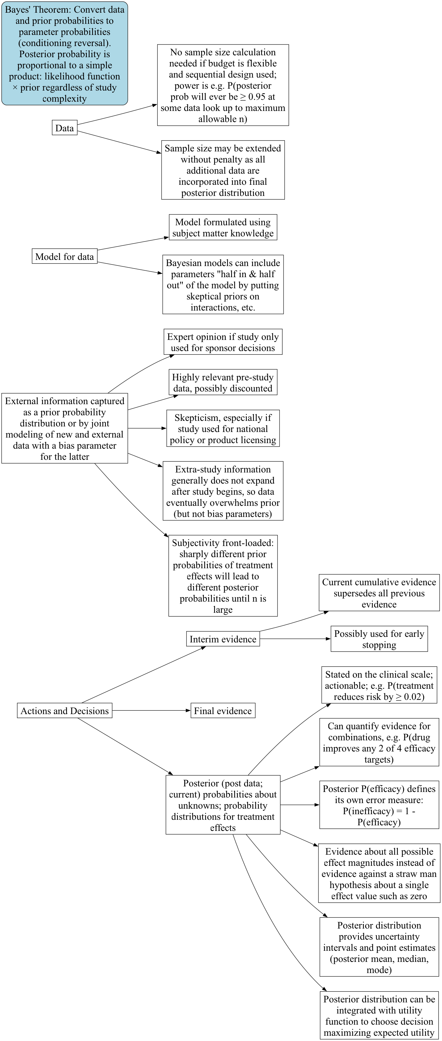
Paradigm Maps: Frequentist | Bayesian
In what appears below1, effect refers to the true unknown treatment effect that generated the observed data, i.e., the systematic signal that needs to be disentangled from all of the random variation. In frequentist parlance this would be called the unknown population treatment effect, and in the Bayesian world is the unknown parameter that is part of the process generating the current dataset, which may in some cases also be a population parameter if repeated sampling were possible (i.e., if a clinical trial could be repeated with no changes in protocol or concomitant therapies). The mode of Bayesian analysis referred to here is posterior analysis using a posterior (“post data”) probability distribution2. In the probability notation below, P(A) means the probability that assertion A is true, and P(A|B) means the conditional probability that A is true given that B is true. Decision refers to playing the odds to maximize the chance of making the right decision analogous to betting decisions made in a round of a card game. Bayesian formal decision analysis, in which the optimal decision is chosen to maximize expected utility, is also available, but requires cost/utility functions that are difficult to specify when there are multiple stakeholders. That approach is not discussed further.
1 Thanks for input from Andrew Hartley of PPD
2 There is another school of Bayesian inference based on Bayes factors which is less flexible and less directly applicable to decision making.
| Concept | Frequentist | Bayesian |
|---|---|---|
| Sample | One of a series of identically distributed samples | Sample may be one of a kind, or replicable |
| Sample size | Maximum sample size usually fixed; selected to achieve a pre-specified power to detect a (usually exaggerated) single effect size | May be left unspecified, or compute an expected sample size; selected to provide pre-specified chance of meeting the study objective, possibly balanced against cost of research |
| Effect | Population effect | Effect generating one dataset, or population effect |
| Probability | Long-run relative frequency; applies only to repeatable experiments | Degree of belief, quantification of veracity, or long-run relative frequency; applies even to one-time events e.g. P(efficacy in context of current concomitant medications) |
| Probabilities computed | Chances about data | Chances about effects that generated the data |
| Goal | Conclusions | Decisions |
| How goal is reached | Infer an assertion is true if assuming it does not lead to a “significant” contradiction | High probability of being correct allows one to act as if an assertion is true whether or not it is true |
| Method of inference | Indirect: assume no effect, attempt proof by contradiction | Direct: compute P(effect | data and prior) |
| Direction of evidence | Evidence against an assertion | Evidence in favor of an assertion |
| Primary evidence measure for fixed \(n\) studies with one data look | p-value: P(another sample would have data more extreme than this study’s | H\(_0\)) | P(efficacy | data, prior) |
| Evidence measure for sequential study | p-value not available; can only use a p-value cutoff \(\alpha^*\) that controls overall type I probability \(\alpha\) | P(efficacy | current cumulative data, prior) |
| Possible error with one data look | \(\alpha\)=Type I: P(data are impressive | no effect) = P(p-value < \(\alpha\)) | P(inefficacy) = 1 - P(effect) |
| Possible error from sequential looks | P(p-value < \(\alpha^*\) | H\(_0\)) at earlier, current, or future looks | current P(inefficacy) = 1 - P(effect) |
| Medical diagnosis analogy | \(\alpha\)=1 - specificity = P(test positive| disease absent) | P(disease is present | test result) |
| External information needed | None, at the cost of indirectness | Directness, at the cost of specifying a prior |
| Objectivity | Objective until translating evidence about data into evidence about effects | Subjective choice of prior, then objective actionability |
| Calculations | Simplified by assuming H\(_0\) when design is simple | Can be complex |
| Calculations required for adaptive or sequential designs | Complex one-off derivations caused by complex sampling distributions | No additional complexity since computing P(effect) not P(data) |
| Sequential trials | Conservative due to penalty for past and future looks | Efficient because looking often at data doesn’t modify how one computes P(effect); older evidence merely superseded by latest data |
| Flexibility | Limited because design adaptations change \(\alpha\) due to opportunities for extreme data | Unlimited within constraints of good science and pre-specification |
| Sample size extension | Complex and requires an \(\alpha\) penalty, making the added patients less informative | Trivial, no penalty |
| Actionability | Unclear since p-values are P(extreme data | no effect) | Probabilities are about quantities of direct clinical interest: P(effect | current information and prior) |