5  Posterior Probabilities With Sequential Analysis

In a Bayesian analysis) It is entirely appropriate to collect data until a point has been proven or disproven, or until the data collector runs out of time, money, or patience. — Edwards et al. (1963)

… sequential designs are often disappointing in what they tell us about the treatment beyond the fact that it works. How well it works is usually not well established. It is sometimes given that the reason that results from sequential trials may be unreliable is precisely because they are sequential. However, I favor a different explanation. They are unreliable when and if they stop early, because in that case, they deliver less information. Many of these difficulties are inherited by flexible designs, and indeed, it has even been claimed that they bring no advantages compared with sequential designs. … I want to make it quite clear that I have no objection with flexible designs where they help us avoid pursuing dead-ends. The analogous technique from the sequential design world is stopping for futility. In my opinion of all the techniques of sequential analysis, this is the most useful. — Senn (2013)

• Bayesian approach allows aggressive sequential testing and early study termination
• Point estimate at termination is pulled back by prior → perfect calibration
• Things go wrong if
  • model incorrectly specified (this also hurts frequentist)
  • prior used in analysis conflicts with prior used by study’s judge
• What if assess efficacy at will and terminate the instant P(efficacy) > 0.95?
• PP on average above 0.95 but remains perfectly calibrated as long as no subtitution of prior
• Math and Bayes’ theorem dictate perfect calibration independent of stopping rule, but simulation exposes logic flow
• Example:
  • one-arm study with maximum n=500
  • look after each subject
  • assume the E raw data measurement with σ=1
  • efficacy = mean μ>0

5.1 Skeptical Prior

• Prior taken to allow harm equally likely as benefits (mean 0)
• Favors no effect (peak of prior density function at 0)
• Low probability of large effects
• Mixtures of normals: flexible way to specify priors
• 1:1 mix of two normals, each with mean 0
• SD of first: P(μ>1)=0.1
• SD of second: P(μ>0.25)=0.05

sd1 <- 1    / qnorm(1 - 0.1)
sd2 <- 0.25 / qnorm(1 - 0.05)

spar(bty='l')
wt  <- 0.5   # 1:1 mixture
pdensity <- function(x) wt * dnorm(x, 0, sd1) + (1 - wt) * dnorm(x, 0, sd2)
x <- seq(-3, 3, length=200)
plot(x, pdensity(x), type='l', xlab=expression(mu), ylab='Prior Density')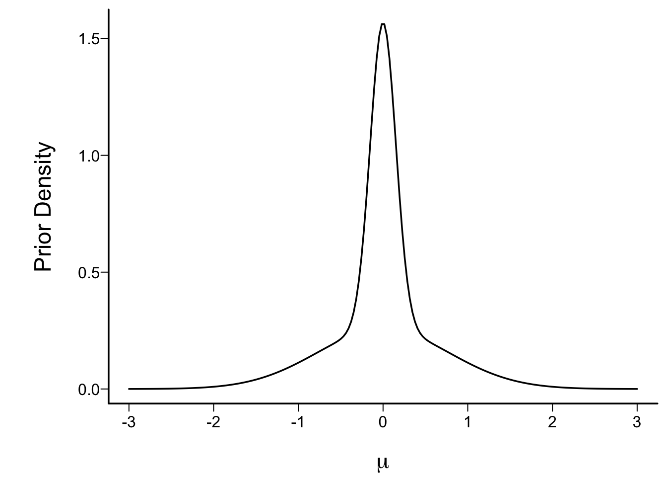

Skeptical prior distribution for the unknown mean in a single arm study. This is a 1:1 mixture of zero mean normals with SD=0.780 and 0.152 respectively.

• Simulate 50,000 different (on μ) studies; reflects real-world case where μ is unknown
• Frequentists emphasize whether if nature throws the null at you, you will not declare the truth non-null
• Bayesian inference: whatever nature throws at you, can we reconstruct what happened?
• Given prior beliefs, Bayes tries to reveal hidden truths by updating your beliefs
• Simulations reflect this:
  • draw μ from the prior
  • generate data assuming that μ
  • do Bayesian analysis that doesn’t know μ but knows the prior generating μ
  • sample sizes analyzed: 1, 2, 3, …, 500
  • for speed, the code generates all 500 data points but they are revealed one-at-a-time
• Stop the instant P(efficacy) ≥ 0.95 or P(futility) ≥ 0.9
• Futility: μ < 0.05

simseq <- function(N, prior.mu=0, prior.sd, wt, mucut=0, mucutf=0.05,
                postcut=0.95, postcutf=0.9,
                ignore=20, nsim=1000) {
  prior.mu <- rep(prior.mu, length=2)
  prior.sd <- rep(prior.sd, length=2)
  sd1 <- prior.sd[1]; sd2 <- prior.sd[2]
  v1 <- sd1 ^ 2
  v2 <- sd2 ^ 2
  j <- 1 : N
  cmean <- Mu <- PostN <- Post <- Postf <- postfe <- postmean <- numeric(nsim)
  stopped <- stoppedi <- stoppedf <- stoppedfu <- stopfe <- status <-
    integer(nsim)
  notignored <- - (1 : ignore)

  # Derive function to compute posterior mean
  pmean <- gbayesMixPost(NA, NA, d0=prior.mu[1], d1=prior.mu[2],
                                 v0=v1, v1=v2, mix=wt, what='postmean')
  
  for(i in 1 : nsim) {
    # See http://stats.stackexchange.com/questions/70855
    component <- if(wt == 1) 1 else sample(1 : 2, size=1, prob=c(wt, 1. - wt))
    mu <- prior.mu[component] + rnorm(1) * prior.sd[component]
    # mu <- rnorm(1, mean=prior.mu, sd=prior.sd) if only 1 component
    
    Mu[i] <- mu
    y  <- rnorm(N, mean=mu, sd=1)
    ybar <- cumsum(y) / j    # all N means for N sequential analyses
    pcdf <- gbayesMixPost(ybar, 1. / j,
                          d0=prior.mu[1], d1=prior.mu[2],
                          v0=v1, v1=v2, mix=wt, what='cdf')
    post  <- 1 - pcdf(mucut)
    PostN[i] <- post[N]
    postf <- pcdf(mucutf)
    s <- stopped[i] <-
      if(max(post) < postcut) N else min(which(post >= postcut))
    Post[i]  <- post[s]   # posterior at stopping
    cmean[i] <- ybar[s]   # observed mean at stopping
    # If want to compute posterior median at stopping:
    #    pcdfs <- pcdf(mseq, x=ybar[s], v=1. / s)
    #    postmed[i] <- approx(pcdfs, mseq, xout=0.5, rule=2)$y
    #    if(abs(postmed[i]) == max(mseq)) stop(paste('program error', i))
    postmean[i] <- pmean(x=ybar[s], v=1. / s)
    
    # Compute stopping time if ignore the first "ignore" looks
    stoppedi[i] <- if(max(post[notignored]) < postcut) N
    else
      ignore + min(which(post[notignored] >= postcut))
    
    # Compute stopping time if also allow to stop for futility:
    # posterior probability mu < 0.05 > 0.9
    stoppedf[i] <- if(max(post) < postcut & max(postf) < postcutf) N
    else
      min(which(post >= postcut | postf >= postcutf))
    
    # Compute stopping time for pure futility analysis
    s <- if(max(postf) < postcutf) N else min(which(postf >= postcutf))
    Postf[i] <- postf[s]
    stoppedfu[i] <- s

    ## Another way to do this: find first look that stopped for either
    ## efficacy or futility.  Record status: 0:not stopped early,
    ## 1:stopped early for futility, 2:stopped early for efficacy
    ## Stopping time: stopfe, post prob at stop: postfe

    stp <- post >= postcut | postf >= postcutf
    s <- stopfe[i] <- if(any(stp)) min(which(stp)) else N
    status[i] <- if(any(stp)) ifelse(postf[s] >= postcutf, 1, 2) else 0
    postfe[i] <- if(any(stp)) ifelse(status[i] == 2, post[s],
                                     postf[s]) else post[N]
  }
  list(mu=Mu, post=Post, postn=PostN, postf=Postf,
       stopped=stopped, stoppedi=stoppedi,
       stoppedf=stoppedf, stoppedfu=stoppedfu,
       cmean=cmean, postmean=postmean,
       postfe=postfe, status=status, stopfe=stopfe)
}

nsim <- 50000
g <- function() {
    set.seed(1)
    simseq(500, prior.mu=0, prior.sd=c(sd1, sd2), wt=wt, postcut=0.95,
           postcutf=0.9, nsim=nsim)
}
z       <- runifChanged(g, sd1, sd2, wt, nsim)
mu      <- z$mu
post    <- z$post
postn   <- z$postn
st      <- z$stopped
sti     <- z$stoppedi
stf     <- z$stoppedf
stfu    <- z$stoppedfu
cmean   <- z$cmean
postmean<- z$postmean
postf   <- z$postf
status  <- z$status
postfe  <- z$postfe
rmean <- function(x) formatNP(mean(x), digits=3)
k  <- status == 2
kf <- status == 1

• 20393 trials stopped early for efficacy, proportion=0.408
  • of 24907 trials with μ>0, proportion=0.786
  • of 2367 trials with μ∈[0.15, 0.2], proportion=0.895
  • of 12210 trials with μ≥0.2, proportion=0.981

• 28438 trials stopped early for futility
• 1169 trials went to completion (n=500)
• Average PP of efficacy at stopping for efficacy: 0.961
• Of trials stopped early for efficacy, proportion with μ > 0: 0.960
• Average PP of futility at stopping for futility: 0.920
• Of trials stopped early for futility, proportion with μ < 0.05: 0.923
• Perfect calibration of PP at stopping point
• Check calibration of P(efficacy) if did not stop for either reason (1169 trials)
  • Assessed using smooth calibration curve exactly as in risk models
  • Relate actual P(μ>0) (from prior) to PP(μ>0)

spar(left=1)
v <- val.prob(postn[status == 0], mu[status == 0] > 0, m=200,
              legendloc=c(.6, .4),
         xlab='Posterior Probability of Efficacy at 500th Look',
         ylab='Proportion of Trials\nwith Efficacy > 0')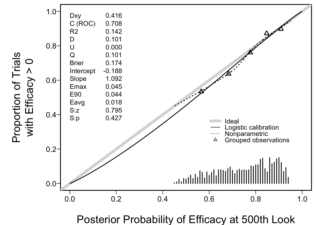

• Histogram showing distribution of true μ when stopped early for efficacy

spar(bty='l')
hist(mu[k], nclass=50, xlim=c(-1,4), xlab='Efficacy', main='')
abline(v=0, col='red', lwd=0.5)
regret <- mean(mu[k] <= 0)
text(-0.5, 500, paste0('Proportion regret=', round(regret, 3)), srt=90, adj=0)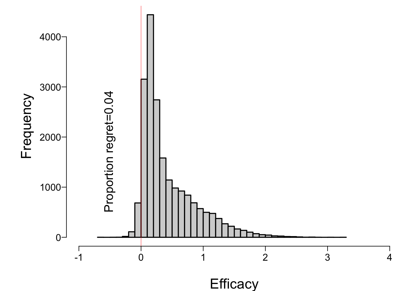

• Check calibration of posterior mean when stop early for efficacy
  • Relate posterior and ordinary sample mean to true μ using “super smoother”

spar(bty='l')
plot(0, 0, xlab='Estimated Efficacy',
     ylab='True Efficacy', type='n', xlim=c(-2, 4), ylim=c(-2, 4))
abline(a=0, b=1, col=gray(.9), lwd=4)
lines(supsmu(cmean[k],    mu[k]))
lines(supsmu(postmean[k], mu[k]), col='blue')
text(2, .4, 'Sample mean')
text(-1, .8, 'Posterior mean', col='blue')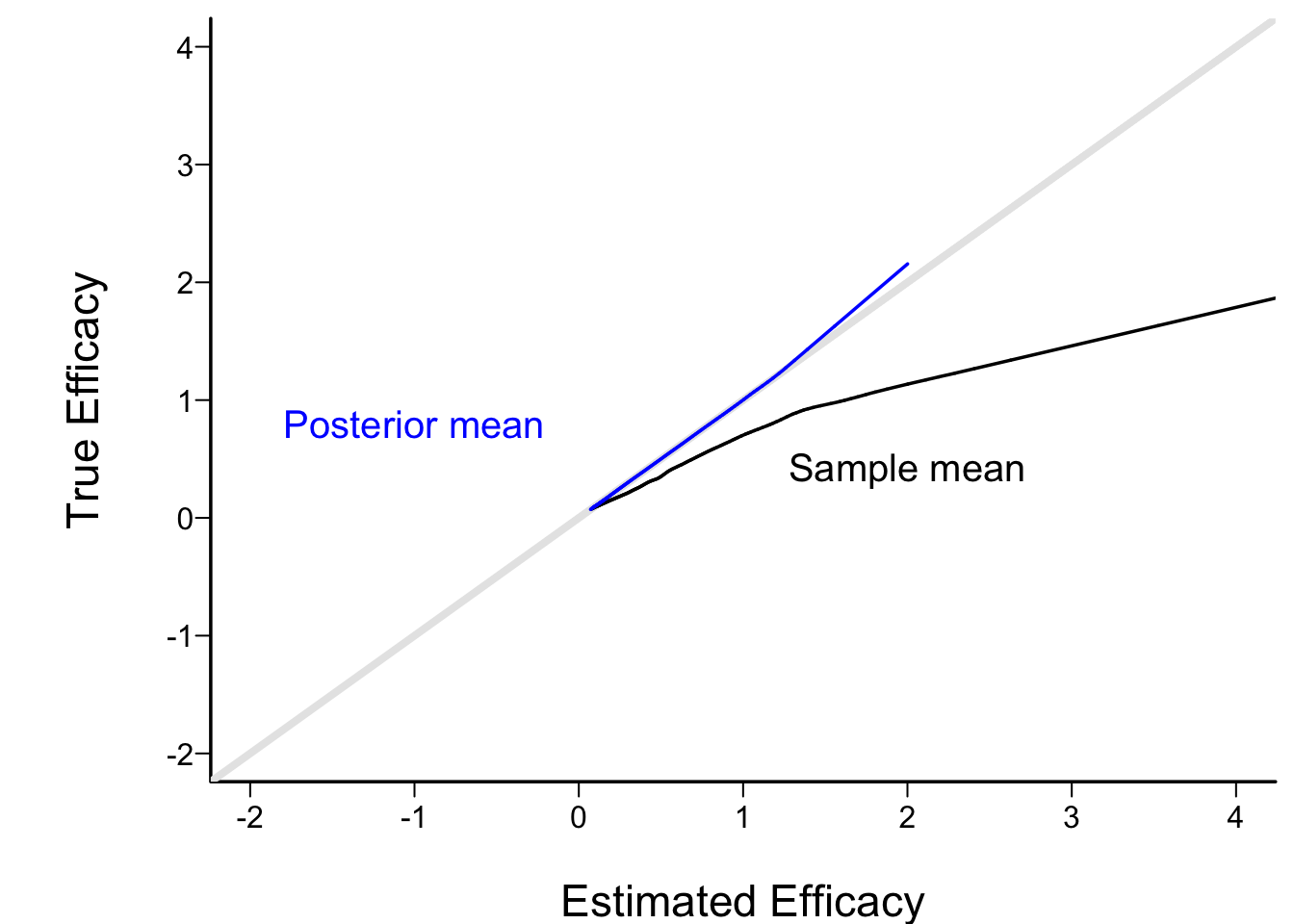

• Frequentist adjustment to sample mean for early stopping is complex, as is CL
• Automatic for Bayesian posterior mean, median, mode, credible interval

Median Stopping Time as a Function of True μ

• Expect to stop earlier when μ generating the data was larger
• Use a parametric survival model (log-normal) to flexibly relate μ to the stopping time
• No early stopping for efficacy → right-censor at sample size of 500

dd <- datadist(mu); options(datadist='dd')
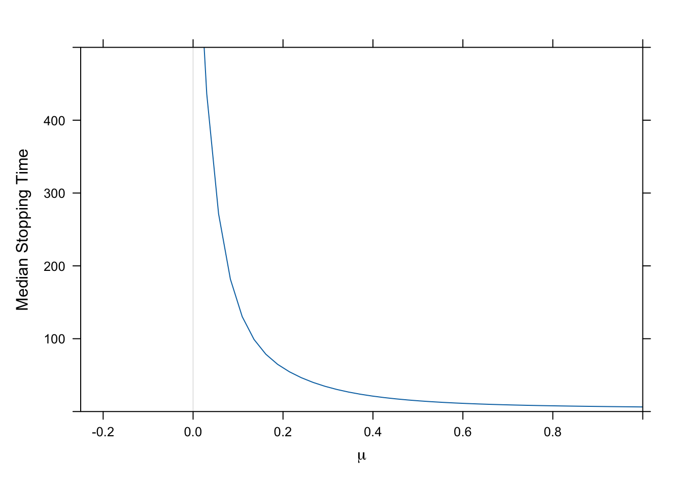
f <- psm(Surv(st, st < 500) ~ rcs(mu, 6), dist='lognormal')
plot(Predict(f, mu, fun=exp, conf.int=FALSE), xlim=c(-.25, 1), ylim=c(0, 500),
     ylab='Median Stopping Time',
     abline=list(list(v=0, col=gray(.9))))

Estimated median stopping time for efficacy as a function of true value of μ, using a log-normal survival time distribution and a restricted cubic spline in μ with 6 default knots. Studies never stopping are right censored at 500 trials.

Edwards, W., Lindman, H., & Savage, L. J. (1963). Bayesian statistical inference for psychological research. Psych Rev, 70(3), 193–242. http://psycnet.apa.org/doi/10.1037/h0044139

Senn, S. (2013). Being Efficient About Efficacy Estimation. Statistics in Biopharmaceutical Research, 5(3), 204–210. https://doi.org/10.1080/19466315.2012.754726

"Every time the statistician working in the pharmaceutical industry does a sample size determination for a trial using a responder analysis, he or she should do the same calculation using the original measure.  If the dichotomy is preferred, an explanation as to why the extra millions are going to be spent should be provided."