    Min      1Q  Median      3Q     Max
-24.580  -4.619   0.154   4.241  24.293
β
S.E.
t
Pr(>|t|)
Intercept
-5.4630
3.6567
-1.49
0.1354
sbp0
1.0048
0.0260
38.62
<0.0001
trt=B
-3.1831
0.3620
-8.79
<0.0001
Code
summary(f)
Effects Response: sbp
Low
High
Δ
Effect
S.E.
Lower 0.95
Upper 0.95
sbp0
135.2
144.5
9.296
9.341
0.2419
8.867
9.816
trt --- B:A
1.0
2.0
-3.183
0.3620
-3.893
-2.473
Code
f <-lrm(ds ~ sbp0 + trt, data=d)f
Logistic Regression Model
lrm(formula = ds ~ sbp0 + trt, data = d)
Model Likelihood
Ratio Test
Discrimination
Indexes
Rank Discrim.
Indexes
Obs 1500
LR χ2 53.82
R2 0.075
C 0.670
0 1357
d.f. 2
R22,1500 0.034
Dxy 0.339
1 143
Pr(>χ2) <0.0001
R22,388.1 0.125
γ 0.339
max |∂log L/∂β| 2×10⁻⁵
Brier 0.083
τa 0.059
β
S.E.
Wald Z
Pr(>|Z|)
Intercept
-15.1566
1.8989
-7.98
<0.0001
sbp0
0.0920
0.0132
6.96
<0.0001
trt=B
-0.2715
0.1807
-1.50
0.1330
Code
summary(f)
Effects Response: ds
Low
High
Δ
Effect
S.E.
Lower 0.95
Upper 0.95
sbp0
135.2
144.5
9.296
0.8549
0.1229
0.6141
1.09600
Odds Ratio
135.2
144.5
9.296
2.3510
1.8480
2.99100
trt --- B:A
1.0
2.0
-0.2715
0.1807
-0.6256
0.08268
Odds Ratio
1.0
2.0
0.7623
0.5349
1.08600
Pearson’s r correlation between the SBP outcome and the death/stroke outcome: 0.22
If frequentist analysis is repeated 2500 times, correlation across the 2500 of the estimated treatment effects on DS and the estimated treatment effects on SBP is 0.142
Bayesian analysis below uses independent models for the two outcomes
Bayesian Analysis
Uses Stan and R rstan package
Regression coefficients have multivariate normal prior with means zero
SD of priors computed so that
P(SBP reduction > 10mmHg) = 0.1
P(OR < 0.5) = 0.05
Residual SD has flat prior on the positive line
Stan No-U-turn sampler in 4 chains with 5,000 post-warmup iterations
20,000 paired posterior draws, took 10m on 4-course machine
        Mean     Median      Lower      Upper
b1 -3.178025 -3.1782677 -3.8796797 -0.5324795
b2 -0.212865 -0.2117236 -0.5324795  0.1025766
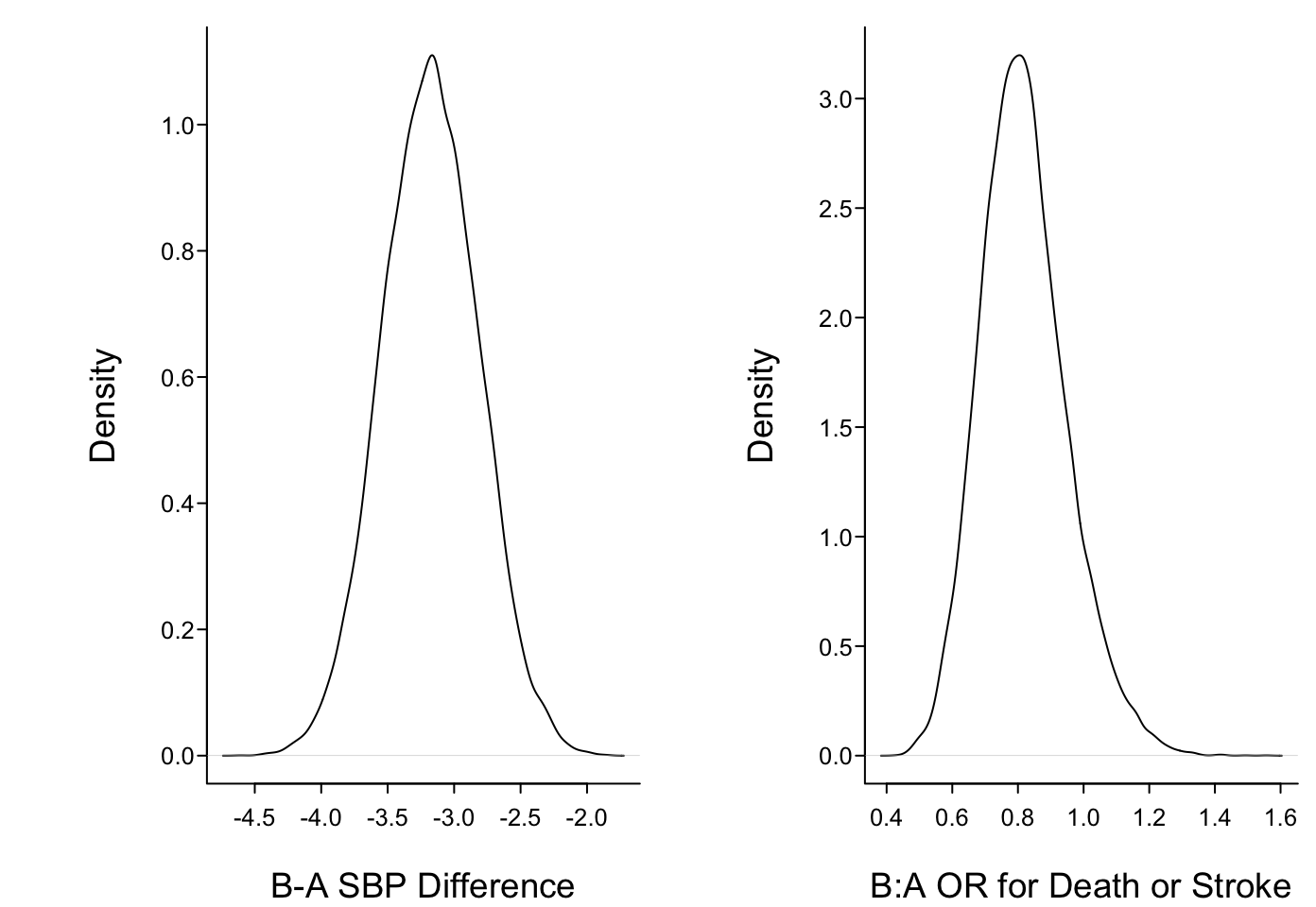
The posterior mean and median log odds ratio is less impressive than the frequentist maximum likelihood estimate of -0.271 because of the skeptical prior
Variety of posterior probabilities easily calculated
Non-inferiority is defined by SBP increase less than 1mmHg and DS increased by an odds ratio less than 1.05
Similarity with respect to effect on DS is an odds ratio between 0.85 and 1/0.85
Final calculation is mean number of targets achieved when the targets are any SBP reduction and any reduction of odds of DS
Code
cat('Prob(SBP reduced at least 2 mmHg) = ', rmean(b1 <-2), '\n','Prob(B:A OR for DS < 1) = ', rmean(b2 <0), '\n','Prob(SBP reduced ≥ 2 and OR < 1) = ', rmean(b1 <-2& b2 <0), '\n','Prob(SBP reduced ≥ 2 or OR < 1) = ', rmean(b1 <-2| b2 <0), '\n','Prob(Non-inferiority) = ', rmean(b1 <1& b2 <log(1.05)),'\n','Prob(DS similar) = ', rmean(exp(b2) >0.85&exp(b2) <1/0.85), '\n','E(# targets achieved) = ', rmean((b1 <0) + (b2 <0)), '\n',sep='')
Prob(SBP reduced at least 2 mmHg) = 0.999
Prob(B:A OR for DS < 1)           = 0.908
Prob(SBP reduced ≥ 2 and OR < 1)  = 0.908
Prob(SBP reduced ≥ 2 or  OR < 1)  = 1.000
Prob(Non-inferiority)             = 0.948
Prob(DS similar)                  = 0.363
E(# targets achieved)             = 1.908
Correlation between the posterior draws is 0.024
6 probabilities above are forward probabilities directly addressing clinical questions
Frequentist solutions for these questions are highly indirect or unavailable
Source Code
```{r echo=FALSE}require(rms)require(qreport)knitr::read_chunk('stan.r')options(prType='html')rmean <-function(x) formatNP(mean(x), digits=3)```# Bayesian Analysis of Simulated RCT with Two Endpoints* Treatments A,B* RCT for hypertension, n=1500* Covariate adjustment for baseline systolic bp* Outcomes + incidence of death or stroke (DS) within 1y<br>binary for illustration, logistic model<br>B:A odds ratio 0.8<br>1y SBP also predicts DS + SBP at 1y, linear model, B:A treatment effect 3mmHg* SBP assumed to be normal with σ=7mmHg given baseline SBP* To estimate population parameters simulate a sample of size n=40,000```{r stansimdatafun}``````{r stansimpop,results='asis'}```* Regression coefficient for treatment when don't adjust for 1y SBP: `r round(btrt, 4)`; B:A odds ratio: `r round(exp(btrt), 4)`* Trial could be run sequentially but we used fixed n=1500 with only one look* Traditional analysis:```{r stansimrct,results='asis'}```* Pearson's r correlation between the SBP outcome and the death/strokeoutcome: `r re`* If frequentist analysis is repeated 2500 times, correlation across the 2500 of the estimated treatment effects on DS and the estimated treatment effects on SBP is 0.142* Bayesian analysis below uses independent models for the two outcomes#### Bayesian Analysis {-}* Uses `Stan` and R `rstan` package* Regression coefficients have multivariate normal prior with means zero* SD of priors computed so that + P(SBP reduction > 10mmHg) = 0.1 + P(OR < 0.5) = 0.05* Residual SD has flat prior on the positive line* Stan No-U-turn sampler in 4 chains with 5,000 post-warmup iterations* 20,000 paired posterior draws, took 10m on 4-course machine```{r stanrun,eval=FALSE}``````{r pstan,echo=FALSE}r <-readLines('stan.lst')cat(r, sep='\n')betas <-readRDS('betas.rds')```* Posterior densities obtained using kernel density estimators```{r postdens}#| fig.width: 7.25#| fig.cap: 'Posterior densities for treatment effects on two outcomes'spar(mfrow=c(1,2), bty='l')b1 <- betas[, 1]b2 <- betas[, 2]plot(density(b1), type='l', xlab='B-A SBP Difference', main='')plot(density(exp(b2)), type='l', xlab='B:A OR for Death or Stroke', main='')```* Posterior means, medians, and 0.95 credible intervals are computed simply by using ordinary samples estimates on the posterior draws```{r stanmcr}ci1 <-quantile(b1, c(0.025, 0.975))ci2 <-quantile(b2, c(0.025, 0.975))data.frame(Mean=c(mean(b1), mean(b2)), Median=c(median(b1), median(b2)),Lower=c(ci1[1], ci2[1]), Upper=c(ci2[1], ci2[2]), row.names=c('b1', 'b2'))```* The posterior mean and median log odds ratio is less impressive than the frequentist maximum likelihood estimate of `r round(coef(f)['trt=B'], 3)` because of the skeptical prior* Variety of posterior probabilities easily calculated* Non-inferiority is defined by SBP increase less than 1mmHg and DS increased by an odds ratio less than 1.05* Similarity with respect to effect on DS is an odds ratio between 0.85 and 1/0.85* Final calculation is mean number of targets achieved when the targets are any SBPreduction and any reduction of odds of DS```{r stanpp}cat('Prob(SBP reduced at least 2 mmHg) = ', rmean(b1 <-2), '\n','Prob(B:A OR for DS < 1) = ', rmean(b2 <0), '\n','Prob(SBP reduced ≥ 2 and OR < 1) = ', rmean(b1 <-2& b2 <0), '\n','Prob(SBP reduced ≥ 2 or OR < 1) = ', rmean(b1 <-2| b2 <0), '\n','Prob(Non-inferiority) = ', rmean(b1 <1& b2 <log(1.05)),'\n','Prob(DS similar) = ', rmean(exp(b2) >0.85&exp(b2) <1/0.85), '\n','E(# targets achieved) = ', rmean((b1 <0) + (b2 <0)), '\n',sep='')```* Correlation between the posterior draws is `r round(cor(b1,b2), 3)`* 6 probabilities above are forward probabilities directly addressing clinical questions* Frequentist solutions for these questions are highly indirect or unavailable