5 Analysis File Creation

flowchart LR
Im[Import] --> vn[Manageable<br>Variable<br>Names] --> An[Annotate<br>Add Metadata]
An --> Int["Internal<br>(imported labels)"] & Ext[External]
An --> lu[Labels<br>Units]
An --> V["View Data Dictionary<br>(metadata)"]
Im --> csv[CSV] & bin[Binary]
Im --> mf[Multiple Files<br>Looping]

5.1 Note on File Directory Structure

I have a directory for each major project, and put everything in that directory (including data files) except for graphics files for figures, which are placed in their own subdirectory underneath the project folder. The directory name for the project includes key identifying information, and files within that directory do not contain project information in their names, nor do they contain dates, unless I want to freeze an old version of an analysis script.

With Quarto I specify that html files are to be self-contained, so there are no separate graphics files.

For multi-analyst projects or ones in which you want to capture the entire code history, having the project on github is worthwhile.

5.2 Importing and Creating Annotated Analysis Files

I typically create a compact analysis file in a separate R script called create.r and have it produce compressed R binary data.frame or data.table .rds files using saveRDS(name, 'name.rds', compress='xz'). Then I have an analysis script named for example a.qmd (for Quarto reports) or a.Rmd (for RMarkdown reports) that starts with d <- readRDS('name.rds'). This process is especially helpful with analysis file creation takes multiple steps or files are large. readRDS is very fast for loading binary R objects, and qread is even faster.

See Section 5.6 for an alternative that is generally preferable to saveRDS using the qs package: qsave(name, 'name.qs') and d <- qread('name.qs').

Templates for analysis reports are here, and a comprehensive report example may be found here.There is an older way to read/write binary R objects using R load and save and Hmisc frontends for them Load and Save. Files using these formats typically have suffixes of .rda, .RData, or .sav, and using load stores the object under its original name, which might not be clear until you check your R .global environment by looking in the upper right RStudio panel.

When variables need to be recoded, have labels added or changed, or have units of measurement added, I specify those using the Hmisc package upData function.

Variable labels and units of measurement are used in special ways in my R packages. This will show up in the describe and contents function outputs below and in axis labels for graphics.

To facilitate some operations requiring variable names to be quoted, the Hmnisc package provides the .q function so that you don’t have to quote names that are legal R object names.

require(Hmisc)
.q(a, b, c, 'this and that')    # same as c('a', 'b', 'c', 'this and that')

[1] "a"             "b"             "c"             "this and that"

.q(dog=a, giraffe=b, cat=c)     # same as c(dog='a', giraffe='b', cat='c')

    dog giraffe     cat 
    "a"     "b"     "c"

Here is an upData example:

# Function to recode from atypical coding for yes/no in raw data
yn <- function(x) factor(x, 0:1, c('yes', 'no'))
d <-
  upData(d,
         rename = .q(gender=sex, any.event=anyEvent),
         posSE    = yn(posSE),
         newMI    = yn(newMI),
         newPTCA  = yn(newPTCA),
         newCABG  = yn(newCABG),
         death    = yn(death),
         hxofHT   = yn(hxofHT),
         hxofDM   = yn(hxofDM),
         hxofCig  = factor(hxofCig, c(0, 0.5, 1),
                           c('heavy', 'moderate', 'non-smoker')), 
         hxofMI   = yn(hxofMI),
         hxofPTCA = yn(hxofPTCA),
         hxofCABG = yn(hxofCABG),
         chestpain= yn(chestpain),
         anyEvent = yn(anyEvent),
         drop=.q(event.no, phat, mics, deltaEF,
                 newpkmphr, gdpkmphr, gdmaxmphr, gddpeakdp, gdmaxdp,
                 hardness),
         labels=c(
           bhr       = 'Basal heart rate',
           basebp    = 'Basal blood pressure',
           basedp    = 'Basal Double Product bhr*basebp',
           age       = 'Age',
           pkhr      = 'Peak heart rate',
           sbp       = 'Systolic blood pressure',
           dp        = 'Double product pkhr*sbp',
           dose      = 'Dose of dobutamine given',
           maxhr     = 'Maximum heart rate',
           pctMphr   = 'Percent maximum predicted heart rate achieved',
           mbp       = 'Maximum blood pressure',
           dpmaxdo   = 'Double product on max dobutamine dose',
           dobdose   = 'Dobutamine dose at max double product',
           baseEF    = 'Baseline cardiac ejection fraction',
           dobEF     = 'Ejection fraction on dobutamine', 
           chestpain = 'Chest pain', 
           ecg       = 'Baseline electrocardiogram diagnosis',
           restwma   = 'Resting wall motion abnormality on echocardiogram', 
           posSE     = 'Positive stress echocardiogram',
           newMI     = 'New myocardial infarction',
           newPTCA   = 'Recent angioplasty',
           newCABG   = 'Recent bypass surgery', 
           hxofHT    = 'History of hypertension', 
           hxofDM    = 'History of diabetes',
           hxofMI    = 'History of myocardial infarction',
           hxofCig   = 'History of smoking',
           hxofPTCA  = 'History of angioplasty',
           hxofCABG  = 'History of coronary artery bypass surgery',
           anyEvent  = 'Death, newMI, newPTCA, or newCABG'),
         units=.q(age=years, bhr=bpm, basebp=mmHg, basedp='bpm*mmHg',
           pkhr=mmHg, sbp=mmHg, dp='bpm*mmHg', maxhr=bpm,
           mbp=mmHg, dpmaxdo='bpm*mmHg', baseEF='%', dobEF='%',
           pctMphr='%', dose=mg, dobdose=mg)
         )

saveRDS(d, 'stressEcho.rds', compress='xz')
# Or qsave(d, 'stressEcho.qs')

# Note that we could have automatically recoded all 0:1 variables
# if they were all to be treated identically:

for(x in names(d)) 
  if(all(d[[x]] %in% c(0,1))) d[[x]] <- yn(d[[x]])

If you want to look up a variable’s comment without having to quote its name use the following:

vcom <- function(...)
  vcomment[as.character(sys.call()[-1])]
# Example usage: vcom(age,sbp,dbp)

Sometimes metadata comes from a separate source. Suppose you imported a data frame d but have also imported a data frame m containing metadata: the same variable names in d (variable name) plus fields label, units, and comment. Dataset m can contain variables not currently being used. To add the labels and units into d and to store comments separately, use the following example.

n <- names(d)
i <- n %nin% m$name
if(any(i)) cat('The following variables have no metadata:',
               paste(n[i], collapse=', '), '\n')
vcomment        <- m$comment
names(vcomment) <- m$name
mn              <- subset(m, name %in% n)
labs            <- mn$label
un              <- mn$units
names(labs)     <- names(un) <- mn$name
d <- upData(d, labels=labs, units=un)

To look up the comment for a variable at any time use e.g. vcomment['height']. All comments were saved in vector vcomment in case the metadata dictionary m defined variables that are not in d but were to be imported later in the script. Comments for multiple variables can be looked up using e.g. vcomment[.q(height, weight, age)].

The R rio package will import most any file type, using mainly the file suffix to determine the type. rio handles files on the web in a unified fashion and also makes file decompression seamless when you access a compressed file archive. It uses the ultra-fast data.table fread function for reading plain-text files such as .csv files.

The Hmisc function fImport is a front-end to rio’s import function that makes it so that variable labels are fully supported by Hmisc and other package’s functions. fImport by default converts imported variable names to lower case when they do not contain mixed case, unless such conversion would result in duplicate variable names. There is an option to convert underscores in variable names to periods.

The built-in function in R for reading .csv files is read.csv. The Hmisc package has a function csv.get which calls read.csv but offers some enhancements in variable naming, date handling, and reading variable labels from a specified row number. Illegal characters in variable names are changed to periods, and by default underscores are also changed to periods. If any variable names are changed and the labels argument is not given, original variable names are stored in the variable label attributes.

Here is an example of using csv.get where the column headings in the first row are better suited as variable labels, and the user has added variable names on the second row. We keep underscores in variable names.

# Create a virtual .csv file
f <-
'Subject ID,Starting Date,Height,Weight
id,sdate,ht,wt_lbs
1,2002-03-07,73,191
2,2007-01-17,68,162
'
require(Hmisc)
# text= is available in csv.get starting with Hmisc 5.0-1
d <- csv.get(text=f, vnames=2, labels=1, skip=2, allow='_')
d

  id      sdate ht wt_lbs
1  1 2002-03-07 73    191
2  2 2007-01-17 68    162

contents(d)


Data frame:d    2 observations and 4 variables    Maximum # NAs:0

              Labels   Class Storage
id        Subject ID integer integer
sdate  Starting Date    Date  double
ht            Height integer integer
wt_lbs        Weight integer integer

The fread function in the data.table package is blazing fast for reading large files and offers a number of options.

If reading data exported from REDCap that are placed into the project directory I run the following to get rid of duplicate (factor and non-factor versions of variables REDCap produces) variables and automatically convert dates to Date variables:

require(Hmisc)
require(qs)
getRs('importREDCap.r')   # source() code to define function
mydata <- importREDCap()  # by default operates on last downloaded export
qsave(mydata, 'mydata.qs')

When file names are not given to importREDCap the function looks for the latest created .csv file and .R file with same prefix and uses those. See this for more information.

getRs('importREDCap.r') also defines the cleanupREDCap function serving several useful roles. It can remove html code (tags) that sometimes clutters variable labels, and it converts sequences representing REDCap multiple choice variables into a single multiple choice variable using the Hmisc package mChoice function to do the work. During the export process, REDCap converts what appears to be one multiple choice entity during data entry into one variable per possible choice, and these variables have names of the form basename___choice number (note the three underscores). Assuming that the checkboxLabels argument to drinkREDCap was set to TRUE if exporting using the REDCap API (see below), cleanupREDCap puts these back into a single variable. Such an mChoice variable has an internal value of, for example, 2;3;7 if choices 2, 3, and 7 were selected for a subject. These are converted to text form if you print the variable, run it through as.character() or format(), or if you run summary() or summaryM() on the variable. For example you may see output in the three choices example of "pain;stomach ache;headache". See mChoice documentation. When the new consolidated variables are created, the original choice variables created by REDCap are removed from the data table. The new variable is the base name of these deleted variables.

You can run cleanupREDCap on a data table d, making changes to it in place using

cleanupREDCap(d, ...)

or you can create a new dataset given a data table or data frame d using

d <- cleanupREDCap(d, ..., byref=FALSE)

The function appends records to a data frame crednotes in the user’s global environment. These records document the changes that importREDCap makes to the input REDCap form. crednotes is set to NULL just before the first append, and the user can run crednotes <- NULL at the top of the script if she wants to ensure that the notes start over if the script is run more than once in an R session.

There are several other features of cleanupREDCap¹:

¹ Many of these features are more automatically handled by the REDCap API, as of 2023-09-01.

By default REDCap labels and levels and the redcapFactor class are removed. You can override this with rmrcl=FALSE.
Set toPOSIXct=TRUE to have all POSIXlt date/time variables to the better POSIXct type.
Specify a vector of variable names in cdatetime to combine separate date and time variables into single date/time variables. Example: cdatetime=.q(visitdate, visittime, lastcontactdate, lastcontacttime).
Specify entrydate and id if you want to convert all date and date/time varibles to be days from entrydate for the corresponding study subject. id is a formula specifying the name of the ID variable in the dataset being processed, and the lookup within entrydate is on the basis of the ID value.
Specify drop as a vector of variable names to drop from the dataset before other processing. Most commonly this will include protected health information. When processing multiple datases, cleanupREDCap accumulates all the names of dropped variables in crednotes. The user can check that every variable named in drop was dropped in at least one dataset using code such as the example below.
Set check=FALSE to suppress checking for dat or tim being in variable names (ignoring case) without the variable officially being a date or time variable. This problem would cause importREDCap to err in processing toPOSIXct and cdatetime and especially entrydate.
Set fixdt to have date, date-time, and time values fixed by converting them to R date/time variables. Another parameter propdt (defaulting to 1/2) specifies the minimum proportion of legal dates/times occurring in a a character variable before it can be considered a date/time. Dates/times are recognized by six different formats (see the cleanupREDCap code for details). fixdt is only applied to variables whose names contain dat (but not data or dati or dat_) or tim. Original illegal values are stored as special missing values and are reported when you run describe().
Specify dsname= a character string form name to have this name recorded in crednotes
Specify mod= a list of functions that are used to transform variables. This is intended to use for restricting identifiability. For example one can truncate zip codes to the first 3 numbers and truncate age at an upper limit of 90. The mod specification for these are as follows (specify mod=phitransform to use these).

ziptrunc <- function(x) {
  if(is.numeric(x)) {
    x <- sprintf('%5s', x)   # right-justified in 5 digits
    x <- gsub(' ', '0', x)   # put leading zeros
    }
  substring(x, 1, 3)
}

phitransform <-
  list('truncate at 90'     = list('age', function(x) pmin(x, 90)),
       'drop last 2 digits' = list('zip', ziptrunc, regex=TRUE) )

The descriptors such as truncate at 90 are recorded in crednotes.

The importREDCap function deals with manually exported files. It would be better to create a reproducible automated workflow in which R makes a request to REDCap and a “live” export of forms in the REDCap database is run. This is facilitated by R package redcapAPI. To install the latest version of the API do the following.

devtools::install_github('vubiostat/redcapAPI', build_vignettes=TRUE)

The process of using the API starts by logging into REDCap and clicking on API on the left panel to fetch your API key. Then when running the API’s unlockREDCap function to unlock files the first time, unlockREDCap will request your API key and ask you for a password. In later runs you will only be requested to provide that password to get access to REDCap files, and in most cases the password is even remembered across R sessions. Those process ensures that sensitive API keys will not appear in your script, so the script can be freely shared or posted publicly.

There is one complication when using the REDCap “longitudinal” model for the database. If you have more than one form, some forms are baseline-only forms, and some are longitudinal, importing all the files at once will result in the baseline-only forms being expanded with many duplicate records per subject. So baseline and longitudinal forms need to be imported separately. In the following example, all baseline-only files are imported at once, and these files are stored in an R list object called B. Then longitudinal files are imported, and stored in list L.

The example code below handles this complication. Before doing that it retrieves all variable-level REDCap metadata for all forms and stores this in data frame meta.

require(redcapAPI)
require(Hmisc)
require(data.table)
getRS('importREDCap.r')   # fetch cleanupREDCap function from Github
api_url<- 'https://redcap..../api/'  # define your server URL

# Unlock two REDCap databases: EDC and Site

unlockREDCap(c(edc_conn  = 'Myproject EDC',
               site_conn = 'Myproject Site Information'),
             keyring = 'API_KEYs',
             envir = globalenv(),   # creates *_conn in global env
             url = api_url)

# Fetch all metadata
meta <- edc_conn$metadata()

# Remove any user-created html from field_label using Hmisc::markupSpecs
meta$field_label <- markupSpecs$html$totxt(meta$field_label)

head(meta)
# Data frame meta contains the following variables: 
# field_name form_name section_header field_type field_label select_choices_or_calculations
# field_note text_validation_type_or_show_slider_number text_validation_min text_validation_max
# identifier branching_logic required_field custom_alignment question_number matrix_group_name
# matrix_ranking field_annotation

# Save date/time stamp for beginning of REDCap export
when <- Sys.time()

# Define a function to fetch a specified list of forms from one database
# If forms are not specified, all forms will be retrieved
# Automatically create mChoice variables and convert character strings
# to dates if > 0.6 of the observations are legal dates
# The result is a list consisting of a collection of forms, and the
# date/time stamp of the data export is added as the 'export_time' attribute
fetch <- function(conn, forms=unique(conn$metadata()$form_name)) {
  if(missing(forms)) {
    cat('\nRetrieving all forms:\n\n')
    print(forms, quote=FALSE)
  }
  d <- exportBulkRecords(list(D=conn),
                         forms=list(D=forms),
                         batch_size=4735,
                         post = function(Records, rcon) {
                           Records |> mChoiceCast(rcon) |>
                             guessDate(rcon, threshold=0.6)})
  names(d) <- sub('^D_', '', names(d))  # Remove D_ prefixes from form names
  attr(d, 'export_time') <- Sys.time()
  d
}

baseline <-
  .q(contact_information,
     consent_documentation,
     demographics,
     pregnancy_assessment,
     inclusionexclusion,
     address_verification,
     randomization,
     pharmacy_confirmation,
     randomization_result,
     shipment_tracking,
     sdv,
     payment_form)

B <- fetch(edc_conn, baseline)

# Make all the baseline data frames data tables with record_id
# as the key.  Remove 4 variables from them

for(n in names(B)) {
  setDT(B[[n]], key='record_id')
  B[[n]][, .q(redcap_event_name, redcap_repeat_instrument,
              redcap_repeat_instance, redcap_survey_identifier) := NULL]
}

# Import longitudinal files

longitudinal <-
  .q(participant_reported_outcomes,
     participant_status,
     pi_data_verification,
     ad_hoc_report,
     healthcare_encounter,
     concomitant_therapy,
     adverse_event_form,
     dcri_sae_report,
     dcri_ae_review,
     participant_contact_log,
     unblinding_request,
     unblinding_result,
     sdv,
     vcc_ctom_unblinding_result,
     notes_to_file,
     results_reporting,
     adjudication)

L <- fetch(edc_conn, longitudinal)

# For all longitudinal forms restructure the event variable and convert
# to data.table with key of record_id and day
# Delete original variable along with redcap_survey_identifier
# Character variable day is made so that alphabetic sorting puts it
# in time order.  This requires putting a leading zero in one-digit days

etrans <- function(event) {
  event     <- sub('_arm_1', '', event)
  event[event == 'screening'] <- 'day_-1'
  sub('day_([1-9])$', 'day_0\\1', event)
}
  
for(n in names(L)) {
  L[[n]]$day <- etrans(L[[n]]$redcap_event_name)
  setDT(L[[n]], key=.q(record_id, day))
    # Do the following if not with drop= for importREDCap
  L[[n]][, .q(redcap_event_name, redcap_survey_identifier) := NULL]
}

L[[1]][, table(day)]

# Put baseline and longitudinal data tables in one large R object
R <- c(B, L)

# Remove html tags from variable labels and convert all sequences
# of multiple choices into single multiple choice variables using
# Hmisc::mChoice.  Use other features of cleanupREDCap too.
# We don't really need the mChoice part since we had the API
# handle this.

# Define combined vector of variables to remove from any dataset
# .q is in Hmisc; May not want to drop the redcap* variables.
drop <- .q(first_name, last_name, email_address, ph_number, addstrt,
           addcity, addstate, addzip5, additional_ph_1, additional_ph_2,
           additional_email, part_addstrt, part_addcity, part_addstate,
           part_addzip5, alt_full_name, alt_ph_number, alt_email,
           redcap_event_name, redcap_repeat_instrument,
           redcap_repeat_instance, redcap_survey_identifier)

# Define date/time variable pairs to be combined
cdt <- .q(visit_date, visit_time, lastcontact_date, lastcontact_time)
# Will drop the time variables and keep the date variables with
# their original names but they will be POSIXct date/time variables

lapply(R, cleanupREDCap, drop=drop, toPOSIXct=TRUE, cdatetime=cdt)

# Check that every variable that was supposed to be
# dropped in >=1 dataset was actually dropped at least once

dropped <- subset(crednotes, description='dropped')$name
j <- drop %nin% dropped.
if(any(j)) cat('Variables never dropped:',
               paste(drop[j], collapse=', '), '\n')

# Save entire database that is in one efficient R object to a
# binary file for fast retrieval
# Add export_time attribute to R to define export date/time
attr(R, 'export_time') <- when
qsave(R, 'R.qs')    # 5.8MB 0.2s
# saveRDS(..., compress='xz') resulted in 3MB R.rds file, 10.7s
# qsave(R, 'R.qs', preset='archive')  resulted in 3.8M, 2.8s

Subsequent programs may retrieve the database using R <- qread('R.qs') and access the export date/time stamp using attr(R, 'export_time').

See the Multiple Files tab for useful R examples for processing multiple files inside objects like the R list just created.

Here are some examples showing how to use mChoice variables.

r <- R$demographics$race_eth
levels(r)   # show all choice descriptions
summary(r)
# Get frequency table of all combinations, numeric form
table(r)
# Same but with labels
table(as.character(r))
# Count number of persons with 'American Indian or Alaska Native'
# as a choice (this was choice # 1)
sum(inmChoice(r, 1))
sum(inmChoice(r, 'American Indian or Alaska Native'))
# Count number of persons in either of two categories
sum(inmChoice(r, c('American Indian or Alaska Native', 'White')))
sum(inmChoice(r, 'White'))
# Count number in both categories
sum(inmChoice(r, c('American Indian or Alaska Native', 'White'),
              condition='all'))
# This is the same as:
sum(inmChoice(r, 'American Indian or Alaska Native') &
    inmChoice(r, 'White'))
# Create a new derived variable for the latter
R$demographics[, aiw := inmChoice(race_eth, c('American Indian or Alaska Native', 'White'),
                                  condition='all')]

SAS, Stata, and SPSS binary files are converted to R data.frames using the R haven package. Here’s an example:

require(haven)   # after you've installed the package
d <- read_sas('mydata.sas7bdat')
d <- read_xpt('mydata.xpt')        # SAS transport files
d <- read_dta('mydata.dta')        # Stata
d <- read_sav('mydata.sav')        # SPSS
d <- read_por('mydata.por')        # Older SPSS files

These import functions carry variable labels into the data frame and convert dates and times appropriately. Character vectors are not converted to factors.

The readxl package that comes with R reads binary Excel spreadsheet .xls and .xlsx files to produce something that is almost a data frame. Here is an example where the imported dataset is converted into a plain data.frame and the variable names are changed to all lower case. read_excel does not handle variable labels. You can specify which sheet or which cell range to import if desired.

d <- readxl::read_excel('my.xlsx')
# Or use require(readxl) then d <- read_excel(...)
d <- as.data.frame(d)
# Or better: make it a data table: setDT(d)
names(d) <- tolower(names(d))

If your spreadsheet has column headings that are more suitable as variable labels, you can use upData to move these labels to become variable names, and save the original column headings as labels. Here is an example where a data frame is constructed that might resemble the imported sheet, then it is transformed.

d <- data.frame('Age in Years'     = c(23, 47), 
                'Cholesterol, mg%' = c(226, 147),
                check.names=FALSE)
d

  Age in Years Cholesterol, mg%
1           23              226
2           47              147

vnames         <- .q(age, chol)    # new variable names, in order
renames        <- vnames
names(renames) <- names(d)
labels         <- names(d)
names(labels)  <- vnames
# Could have done
#  renames <- structure(vnames,   names=names(d))
#  labels  <- structure(names(d), names=vnames)
renames

    Age in Years Cholesterol, mg% 
           "age"           "chol"

labels

               age               chol 
    "Age in Years" "Cholesterol, mg%"

d <- upData(d, rename=renames, labels=labels)

Input object size:   912 bytes;  2 variables     2 observations
Renamed variable     Age in Years   to age 
Renamed variable     Cholesterol, mg%   to chol 
New object size:    1936 bytes; 2 variables 2 observations

  age chol
1  23  226
2  47  147

contents(d)


Data frame:d    2 observations and 2 variables    Maximum # NAs:0

               Labels   Class Storage
age      Age in Years integer integer
chol Cholesterol, mg% integer integer

One of the most important principles to following in programming data analyses is to not do the same thing more than once. Repetitive code wastes time and is harder to maintain. One example of avoiding repetition is in reading a large number of files in R. If the files are stored in one directory and have a consistent file naming scheme (or you want to import every .csv file in the directory), one can avoid naming the individual files. The results may be stored in an R list that has named elements, and there are many processing tasks that can be automated by looping over this list.

In the following example assume that all the data files are .csv files in the current working directory, and they all have names of the form xz*.csv. Let’s read all of them and put each file into a data frame named by the characters in front of .csv. These data frames are stuffed into a list named X. The Hmisc csv.get function is used to read the files, automatically translating dates to Date variables, and because lowernames=TRUE is specified, variable names are translated to lower case. There is an option to fetch variable labels from a certain row of each .csv file but we are not using that.

files <- list.files(pattern='xz.*.csv')  # vector of qualifying file names
# Get base part of *.csv
dnames <- sub('.csv', '', files)
X <- list()
i <- 0
for(f in files) {
  cat('Reading file', f, '\n')
  i <- i + 1
  d <- csv.get(f, lowernames=TRUE)
  # To read SAS, Stata, SPSS binary files use a haven function instead
  # To convert to data.table do setDT(d) here
  X[[dnames[i]]] <- d
}
saveRDS(X, 'X.rds', compress='xz')  # Efficiently store all datasets together
# Or qsave(X, 'X.qs')

To process one of the datasets one can do things like summary(X[[3]]) or summary(X$baseline) where the third dataset stored was named baseline because it was imported from baseline.csv.

Now there are many possibilities for processing all the datasets at once such as the following.

names(X)                  # print names of all datasets
k   <- length(X)          # number of datasets
nam <- lapply(X, names)   # list with k elements, each is a vector of names
# Get the union of all variable names used in any dataset
sort(unique(unlist(nam))) # all the variables appearing in any dataset
# Get variable names contained in all datasets
common <- names(X[[1]])
for(i in 2 : k) {
  common <- intersect(common, names(X[[i]]))
  if(! length(common)) break  # intersection already empty
}
sort(common)
# Compute number of variables across datasets
nvar <- sapply(X, length)  # or ncol
# Print number of observations per dataset
sapply(X, nrow)
# For each variable name count the number of datasets containing it
w <- data.table(dsname=rep(names(X), nvar), vname=unlist(nam))
w[, .N, keyby=vname]
# For each variable create a comma-separated list of datasets
# containing it
w[, .(datasets=paste(sort(dsname), collapse=', ')), keyby=vname]
# For datasets having a subject ID variable named id compute
# the number of unique ids
uid <- function(d) if('id' %in% names(d)) uniqueN(d$id) else NA
sapply(X, uid)
# To repeatedly analyze one of the datasets, extract it to a single data frame
d <- X$baseline
describe(d)

Most of these steps are automated in the qreport package multDataOverview function.

require(qreport)   # if not done already
m <- multDataOverview(X, ~ id)  # Leave off m <- if not needing to print m
# To print a long table showing all the datasets containing each variable,
# print m
m

Sometimes one keeps multiple versions of the raw data to be imported inside the project folder. If you want to import the file that was last modified you can use the Hmisc package latestFile function. You give it a pattern of file names to match. For example a pattern of .csv$ means “ending with .csv” and a pattern of ^baseline means “starting with baseline”. A pattern of foo means that foo is contained anywhere in the file name. Here is an example.

# Look for file names starting with base, followed by any number of
# characters, and ending with .csv
f <- latestFile('^base.*csv$')
d <- csv.get(f)

The Hmisc package cleanup.import function improves imported data storage in a number of ways including converting double precision variables to integer when originally double but not containing fractional values (this halves the storage requirement). cleanup.import has an argument moveUnits to extract units of measurements from labels (if enclosed in parentheses or brackets) and move them to units attributes. Hmisc::upData is the go-to function for annotating data frames/tables, renaming variables, and dropping variables. Hmisc::dataframeReduced removes problematic variables, e.g., those with a high fraction of missing values or that are binary with very small prevalence.

5.3 Variable Naming

I prefer short but descriptive variable names. As exemplified above, I use variable labels and units to provide more information. For example I wouldn’t name the age variable age.at.enrollment.yrs but would name it age with a label of Age at Enrollment and with units of years. Short, clear names unclutter code, especially formulas in statistical models. One can always fetch a variable label while writing a program (e.g., typing label(d$age) at the console) to check that you have the right variable (or put the data dictionary in a window for easy reference, as shown below). Hmisc package graphics and table making functions such as summaryM and summary.formula specially typeset units in a smaller font.

When the current dataset is named d or you run options(current_ds='dataset name') or have run the Hmisc extractlabs function, you can retrieve labels and units even easier while in the console. Using the Hmisc vlab function you can just type vlab(age).

5.4 Data Dictionary

The Hmisc package contents function will provide a concise data dictionary. Here is an example using the permanent version (which coded binary variables as 0/1 instead of N/Y) of the dataset created above, which can be accessed with the Hmisc getHdata function. The top of the contents output has the number of levels for factor variables hyperlinked. Click on the number to go directly to the list of levels for that variable.

require(Hmisc)
options(prType='html')
getHdata(stressEcho)
d <- stressEcho

Data Dictionary

contents(d)

d Contents

Data frame:d

558 observations and 31 variables, maximum # NAs:0

Name	Labels	Units	Levels	Storage
bhr	Basal heart rate	bpm		integer
basebp	Basal blood pressure	mmHg		integer
basedp	Basal Double Product bhr*basebp	bpm*mmHg		integer
pkhr	Peak heart rate	mmHg		integer
sbp	Systolic blood pressure	mmHg		integer
dp	Double product pkhr*sbp	bpm*mmHg		integer
dose	Dose of dobutamine given	mg		integer
maxhr	Maximum heart rate	bpm		integer
pctMphr	Percent maximum predicted heart rate achieved	%		integer
mbp	Maximum blood pressure	mmHg		integer
dpmaxdo	Double product on max dobutamine dose	bpm*mmHg		integer
dobdose	Dobutamine dose at max double product	mg		integer
age	Age	years		integer
gender			2	integer
baseEF	Baseline cardiac ejection fraction	%		integer
dobEF	Ejection fraction on dobutamine	%		integer
chestpain	Chest pain			integer
restwma	Resting wall motion abnormality on echocardiogram			integer
posSE	Positive stress echocardiogram			integer
newMI	New myocardial infarction			integer
newPTCA	Recent angioplasty			integer
newCABG	Recent bypass surgery			integer
death				integer
hxofHT	History of hypertension			integer
hxofDM	History of diabetes			integer
hxofCig	History of smoking		3	integer
hxofMI	History of myocardial infarction			integer
hxofPTCA	History of angioplasty			integer
hxofCABG	History of coronary artery bypass surgery			integer
any.event	Death, newMI, newPTCA, or newCABG			integer
ecg	Baseline electrocardiogram diagnosis		3	integer

Category Levels

gender

male

female

hxofCig

heavy

moderate

non-smoker

ecg

normal

equivocal

You can write the text output of contents into a text file in your current working directory, and click on that file in the RStudio Files window to create a new tab in the editor panel where you can view the data dictionary at any time. This is especially helpful if you need a reminder of variable definitions that are stored in the variable labels. Here is an example where the formatted data dictionary is saved.

Users having the xless system command installed can pop up a contents window at any time by typing xless(contents(d)) in the console. xless is in Hmisc.

capture.output(contents(d), file='contents.txt')

Or put the html version of the data dictionary into a small browser window to which you can refer at any point in analysis coding.

cat(html(contents(d)), file='contents.html')
browseURL('contents.html', browser='vivaldi -new-window')

RStudio provides a nice way to do this, facilitated by the htmlView helper function in qreport. htmlView takes any number of objects for which an html method exists to render them. They are rendered in the RStudio Viewer pane. If you are running outside RStudio, your default browser will be launched instead.

Occasionally RStudio Viewer will drop its arrow button making it impossible to navigate back and forth to different html outputs.

require(qreport)
# Defines htmlView, htmlViewx, kabl, maketabs, dataChk, ...
htmlView(contents(d))

In some cases it is best to have a browser window open to the full descriptive statistics for a data table/frame (see below; the describe function also shows labels, units, and levels).

For either approach it would be easy to have multiple tabs open, one tab for each of a series of data tables, or use htmlView.

To be able to have multiple windows open to see information about datasets it is advantageous to open an external browser window. The htmlViewx function will by default open a Vivaldi browser window with the first output put in a new window and all subsequent objects displayed as tabs within that same window. This behavior can be controlled with the tab argument, and you can use a different browser by issuing for example options(vbrowser='firefox'). As an example suppose that two datasets were read from the hbiostat.org/data data repository, and the data dictionary and descriptive statistics for both datasets were to be converted to html and placed in an external browser window for the duration of the R session.

In Windows you may have to specify a full path and firefox.exe.

getHdata(support)
getHdata(support2)
htmlViewx(contents(support ), describe(support ),
          contents(support2), describe(support2))

A screenshot of the result is here.

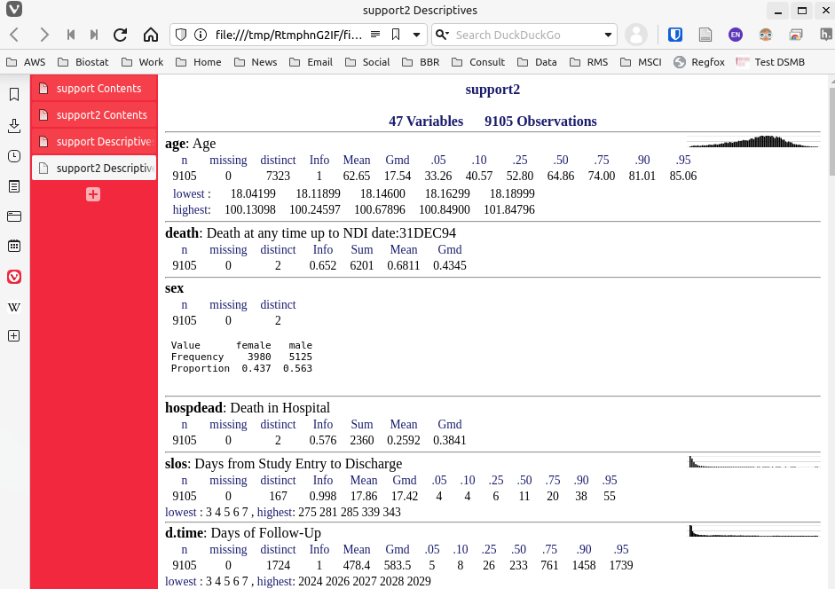
But for the majority of situations you can just let R automatically route the outputs of contents() and describe() to the Viewer when running from the console or running one line of code at a time in the script editor window. This assumes that options(prType='html') is in effect.

5.5 Efficient Storage and Retrieval With `fst`

The fst package of Mark Klik provides an incredibly efficient way to write and read binary files holding R data frames or data tables. For very large files, fst adds efficiency by providing fast direct access of selected rows and/or columns. The only downside is that fst drops user-added attributes of columns, e.g. units and label. So we need to use the Hmisc keepHattrib and restoreHattrib functions to save such attributes in a separate object and to apply them back to the data frame/table after running read_fst. Here is an example for a 10,000,000 row data table with three columns.

See Section 10.9 for more examples of the fst package.

require(data.table)
require(fst)
d <- data.table(a=runif(1e7), b=rnorm(1e7),
                f=factor(sample(c('a','b','c'), 1e7, replace=TRUE)))
d <- upData(d, labels=c(a='A', b='B', f='F'), units=c(b='cm'))

Input object size:   200002128 bytes;    3 variables     10000000 observations
New object size:    200003688 bytes;    3 variables 10000000 observations

at <- keepHattrib(d)
# The following took 1.5s (0.16s with default compress=50 but .fst file 1.5x larger)
write_fst(d,  '/tmp/d.fst',  compress=100)     # maximum compression
saveRDS(at, '/tmp/at.rds',   compress='xz')    # not a data frame; can't use fst
dr  <- read_fst('/tmp/d.fst', as.data.table=TRUE)  # 0.06s (0.03s with compress=50)
atr <- readRDS('/tmp/at.rds')
contents(dr)

dr Contents

Data frame:dr

10000000 observations and 3 variables, maximum # NAs:0

Name	Levels	Storage
a		double
b		double
f	3	integer

Category Levels

f

dr <- restoreHattrib(dr, atr)
contents(dr)

dr Contents

Data frame:dr

10000000 observations and 3 variables, maximum # NAs:0

Name	Labels	Units	Levels	Class	Storage
a	A			numeric	double
b	B	cm		numeric	double
f	F		3		integer

Category Levels

f

A pair of functions to automate this process is found in the saveRfiles script on github. Here is how this streamlines what is above. Let’s also show how to retrieve only a subset of the data table (two columns and only the first 1000 rows).

getRs('saveRfiles.r')
save_fst(d)

Data saved in d.fst and attributes saved in d-attr.rds

# In the next line the value of d is not used but d is used
# for the base file name
dr <- retrieve_fst(d, as.data.table=TRUE,
                   columns=.q(a, b), from=1, to=1000)
contents(dr)

dr Contents

Data frame:dr

1000 observations and 2 variables, maximum # NAs:0

Name	Labels	Units	Class	Storage
a	A		numeric	double
b	B	cm	numeric	double

invisible(file.remove('d.fst', 'd-attr.rds'))

5.6 Efficient Storage and Retrieval With `qs`

The qs package, like fst, provides fast reading and writing of R objects. Unlike fst, qs can store any type of object, does not lose attributes, and does not allow for direct access of selected rows or columns. Let’s compare qs, fst, and saveRDS for speed and disk storage efficiency. First, make sure that qs keeps all attributes.

require(qs)
getHdata(support)   # loads from hbiostat.org/data; has
                    # lots of variable attributes
qsave(support, '/tmp/support.qs')
w <- qread('/tmp/support.qs')
identical(support, w)

[1] TRUE

Now try some things on the 10,000,000 row data table created above.

saveRDS(d, '/tmp/d.rds')                  # 13.6s 128M
saveRDS(d, '/tmp/dc.rds', compress='xz')  #  124s 116M
write_fst(d, '/tmp/d.fst')                #  0.2s 161M
write_fst(d, '/tmp/dc.fst', compress=100) #  1.4s 122M
qsave(d, '/tmp/d.qs', nthreads=3)         #  0.3s 110M

Read times are as follows.

readRDS('/tmp/d.rds')           # 0.9 s
readRDS('/tmp/dc.rds')          # 7.5 s
read_fst('/tmp/d.fst')          # 0.04s
read_fst('/tmp/dc.fst')         # 0.07s
qread('/tmp/d.qs')              # 0.2 s
qread('/tmp/d.qs', nthreads=6)  # 0.16s

When direct access is not needed, i.e., when whole data frames/tables are to be read, the qs package would be a good default, especially if one takes into account that qs preserves all object attributes. qs dependencies are also more actively supported.

5.7 Secure File Storage and Transmission

Sometimes files contain sensitive information such as personal identifiers, addresses, phone numbers, or government ID numbers. Be aware of local rules for storage of files containing such information. My institution requires encrypting disks containing such files. Even if you don’t need protection locally, you may need to transmit sensitive files and need to prevent damage from them falling into the wrong hands. A way to do this is to encrypt data files that your R script outputs to disk, using a secure password for encryption and decryption, and sharing the password safely.

The Hmisc package has a function qcrypt that greatly simplifies a workflow to protect stored data. This workflow has the following features:

qcrypt is available as of Hmisc 5.1-1 and may be obtained here until that version is available in CRAN.

System keyrings are used to cache passwords, and the creator of the file is asked for the password only once (possibly again if rebooting the computer or otherwise starting a new session); handled by the keyring package
Passwords do not appear in R code but are entered into a pop-up window; done by the getPass package
Objects are saved externally in a very efficient manner using the qs package (see above)
The saved unencrypted file exists only momentarily in a temporary directory
The file is encrypted and saved in the current working directory using the safer package and the unencrypted file is immediately deleted
When a stored file is decrypted, the decrypted .qs file is stored only momentarily in a temporary directory, and is deleted once the unencrypted file is read using qs::qread.

The overhead of encrypting and decrypting is small, e.g., 0.5s for a data frame with 100,000 rows and 100 columns.

Here is an example using qcrypt to encrypt and then to decrypt a data frame. The decryption phase can appear in a different script and the password will still be cached.

x <- data.frame(...)
qcrypt(x, 'x')
x <- qcrypt('x')

1: Asks for a password (one-time); use qs::qsave to create a temporary file x.qs in a temporary directory; store encrypted version as x.qs.encrypted in current working directory; delete x.qs
2: Unencrypt x.qs.encrypted into a temporary directory as x.qs using the cached password; use qs::qread to read it; store the result in x

qcrypt also has the capability to encrypt general files such as html and pdf reports and csv files.

The safer package can encrypt/decrypt R objects and general files. qcrypt did not use safer’s object encryption capabilities because in a test the resulting .qs file was much larger due to originally sparse data not being sparse any more upon encryption.

The functions that qcrypt calls may only be called in an interactive R session. If you want to be able to run the main part (e.g., main.qmd) of a script in batch mode, create an interactive script like the following. If your operating system does not have a /tmp directory for storing temporary files, use another appropriate directory name.

require(Hmisc)
require(qs)

w <- qcrypt('w')                    # reads w.qs.encrypted
qsave(w, '/tmp/w.qs')

system('quarto render main.qmd')    # creates /tmp/u.qs

u <- qread('/tmp/u.qs')
qcrypt(u, 'u')                      # writes u.qs.encrypted

unlink(c('/tmp/w.qs', '/tmp/u.qs')) # remove temporary files

5.7.1 Depositing Files on `REDCap`

Users of REDCap have access to a file repository attached to each of their projects. This is often used to store documentation files but can also be used to securely store analysis files created by R that others who have project access can download. Thanks to an API and the R RCurl package, files can be automatically uploaded in R. An API token is retreived from REDCap. This token applies to a particular subdirectory in the project’s file repository, and uploads will put files in that subdirectory. If a file by the same name already exists, the newly uploaded file will have a sequential version number added to the file name. The user may wish to delete old files before running R so that this doesn’t happen.

Here is a function that makes it easy to write files to the repository.

upload <- function(file) {
  RCurl::postForm('https://redcap..../api/',   # specify your REDCap server
           token='put token for subdirectory here',
           content='fileRepository',
           action='import',
           returnFormat='csv',  # for example
           folder_id='52',
           file=RCurl::fileUpload(file))
}

upload('my.csv')

5.1 Note on File Directory Structure

5.2 Importing and Creating Annotated Analysis Files

5.3 Variable Naming

5.4 Data Dictionary

Data frame:d

Category Levels

gender

hxofCig

ecg

5.5 Efficient Storage and Retrieval With fst

Data frame:dr

Category Levels

f

Data frame:dr

Category Levels

f

Data frame:dr

5.6 Efficient Storage and Retrieval With qs

5.7 Secure File Storage and Transmission

5.7.1 Depositing Files on REDCap

5.5 Efficient Storage and Retrieval With `fst`

5.6 Efficient Storage and Retrieval With `qs`

5.7.1 Depositing Files on `REDCap`