flowchart LR
sf[Storage Formats]
sf1[Tree]
sf2[Short and Wide]
sf3[Tall and Thin]
sf3a[Uniform Number<br>of Rows,<br>With NAs]
sf3b[Variable Number<br>of Rows,<br>With Few NAs]
sf --> sf1 & sf2 & sf3
sf3 --> sf3a & sf3b
locf[Last<br>Observation<br>Carried<br>Forward]
crr[Carry<br>Forward<br>by Adding<br>Rows]
fi[Find First<br>Observation<br>Meeting Criteria]
cf[Using Functions<br>That Count<br>Criteria Met]
im[Inexact<br>Matching]
sf3a --> locf
sf3b --> crr & fi & cf & im
13 Manipulation of Longitudinal Data
The data.table package provides exceptional capabilities for manipulating longitudinal data, especially when performing operations by subject. Before showing a variety of examples that typify common tasks, consider that there are many ways to store longitudinal data, including
- as an R
listhierarchical tree with one branch per subject (not considered here) - “short and wide” with one column per time point (not considered here because this setup requires much more metadata setup, more storage space, and more coding)
- “tall and thin” with one row per subject per time point observed (the primary format considered in this chapter; typically there are few
NAs unless many response variables are collected at a single time and some of them areNA) - “tall and thin” with one row per subject per time point potentially observed, with missing values (
NA) for unobserved measurements (considered in the first example)
Here are some useful guidelines for making the most of data.table when processing longitudinal data. These elements are used in many of the examples in this chapter.
- Minimize the use of
$ - Don’t use
forloops or*apply - Write a little function that does what you need for one subject then incorporate that function inside
DT[…]after running a variety of tests on the function, for one subject at a time. Be sure to test edge cases such as there being no non-NAvalues for a subject. - Think generally. One of the examples in this chapter used run length encoding to make a function to count how many conditions are satisfied in a row (over time). That kind of counting function allows you to do all kinds of things elegantly.
13.1 Uniform Number of Rows
Consider first the case where most of the subjects have the same number of rows and NA is used as a placeholder with a certain measurement is not made on a given time. Though highly questionable statistically, last observation carried forward (LOCF) is sometimes used to fill in NAs so that simple analyses can be performed.
LOCF is a form of missing value imputation where imputed values are treated the same as real measurements, resulting in highly deflated estimates of standard errors and much higher than nominal \(\alpha\) in frequentist statistical testing.
data.table has an efficient built-in functions for LOCF (and for last observation carried backward and fill-in using a constant value): nafill and setnafill. Consider a longitudinal data table L with 5 observations per each of two subjects.
require(Hmisc)
require(data.table)
require(ggplot2)
L <- data.table(id  = c(1, 1, 1, 1, 1, 2, 2, 2, 2, 2),
                day = c(1, 2, 3, 4, 5, 1, 2, 3, 4, 5),
                y1  = 1:10,
                y2  = c(NA, 1, NA, NA, 2, 1, 2, 3, 4, NA),
                key = .q(id, day))
# .q(id, day) is the Hmisc version of c('id', 'day')
L
Key: <id, day>
id day y1 y2
<num> <num> <int> <num>
1: 1 1 1 NA
2: 1 2 2 1
3: 1 3 3 NA
4: 1 4 4 NA
5: 1 5 5 2
6: 2 1 6 1
7: 2 2 7 2
8: 2 3 8 3
9: 2 4 9 4
10: 2 5 10 NAsetnafill(L, "locf", cols=.q(y1, y2))
LKey: <id, day>
id day y1 y2
<num> <num> <int> <num>
1: 1 1 1 NA
2: 1 2 2 1
3: 1 3 3 1
4: 1 4 4 1
5: 1 5 5 2
6: 2 1 6 1
7: 2 2 7 2
8: 2 3 8 3
9: 2 4 9 4
10: 2 5 10 4setnafill changed the data table in place. Note that y1 is unchanged since it contained no NAs.
13.2 Variable Number of Rows
Consider the somewhat more frequently occuring situation where there is one row per subject per time at which a measurement is made. Consider a different data table L, and create records to fill out the observations, carrying forward to 4 days the subject’s last observation on y if it was assessed earlier than day 4.
L <- data.table(id = c(2, 2, 2, 3, 3, 3, 3, 4, 4, 5, 5, 5),
day = c(1, 2, 3, 1, 2, 3, 4, 1, 2, 1, 2, 3),
y = 1 : 12, key='id')
w <- copy(L)
u <- w[, .q(seq, maxseq) := .(1 : .N, .N),
by=id][
seq == maxseq & day < 4,]
u <- u[, .(day = (day + 1) : 4, y = y), by=id]
u
w <- rbind(L, u, fill=TRUE)
setkey(w, id, day)
w- 1
-
fresh start with no propagation of changes back to
L. Only needed if will be using:=to compute variables in-place and you don’t want the new variables also added toL. This is related to data.table doing things by reference instead of making copies.w <- Ldoes not create new memory forw. - 2
-
within one subject compute consecutive record numbers
1 : .Nand last record number.N - 3
- separately by subject
- 4
-
feed this result directly into a
data.tableoperation to save last records when the last record is on a day before day 4 - 5
- fill out to day 4 by adding extra observations, separately by subject
- 6
-
vertically combine observations in
Landu, filling variables missing from one of the data tables with missing values (NA) - 7
-
sort by subject
idanddaywithinidand set these variables as dataset keys
Key: <id>
      id   day     y
   <num> <int> <int>
1:     2     4     3
2:     4     3     9
3:     4     4     9
4:     5     4    12
Key: <id, day>
       id   day     y
    <num> <num> <int>
 1:     2     1     1
 2:     2     2     2
 3:     2     3     3
 4:     2     4     3
 5:     3     1     4
 6:     3     2     5
 7:     3     3     6
 8:     3     4     7
 9:     4     1     8
10:     4     2     9
11:     4     3     9
12:     4     4     9
13:     5     1    10
14:     5     2    11
15:     5     3    12
16:     5     4    12
Find the first time at which y >= 3 and at which y >= 7.
day[y >= 3] is read as “the value of day when y >= 3”. It is a standard subscripting operation in R for two parallel vectors day and y. Taking the minimum value of day satisfying the condition gives us the first qualifying day.L[, .(first3 = min(day[y >= 3]),
first7 = min(day[y >= 7])), by=id]Key: <id>
id first3 first7
<num> <num> <num>
1: 2 3 Inf
2: 3 1 4
3: 4 1 1
4: 5 1 1Same but instead of resulting in an infinite value if no observations for a subject meet the condition, make the result NA.
mn <- function(x) if(length(x)) min(x) else as.double(NA)
# as.double needed because day is stored as double precision
# (type contents(L) to see this) and data.table requires
# consistent storage types
L[, .(first3 = mn(day[y >= 3]),
      first7 = mn(day[y >= 7])), by=id]
Key: <id>
id first3 first7
<num> <num> <num>
1: 2 3 NA
2: 3 1 4
3: 4 1 1
4: 5 1 1Add a new variable z and compute the first day at which z is above 0.5 for two days in a row for the subject. Note that the logic below looks for consecutive days for which records exist for a subject. To also require the days to be one day apart add the clause day == shift(day) + 1 after shift(z) > 0.5.
set.seed(1)
w <- copy(L)
w[, z := round(runif(.N), 3)]
u <- copy(w)
u
Key: <id>
id day y z
<num> <num> <int> <num>
1: 2 1 1 0.266
2: 2 2 2 0.372
3: 2 3 3 0.573
4: 3 1 4 0.908
5: 3 2 5 0.202
6: 3 3 6 0.898
7: 3 4 7 0.945
8: 4 1 8 0.661
9: 4 2 9 0.629
10: 5 1 10 0.062
11: 5 2 11 0.206
12: 5 3 12 0.177mn <- function(x)
if(! length(x) || all(is.na(x))) as.double(NA) else min(x, na.rm=TRUE)
u[, consecutive := z > 0.5 & shift(z) > 0.5, by=id][,
firstday := mn(day[consecutive]), by=id]
uKey: <id>
id day y z consecutive firstday
<num> <num> <int> <num> <lgcl> <num>
1: 2 1 1 0.266 FALSE NA
2: 2 2 2 0.372 FALSE NA
3: 2 3 3 0.573 FALSE NA
4: 3 1 4 0.908 NA 4
5: 3 2 5 0.202 FALSE 4
6: 3 3 6 0.898 FALSE 4
7: 3 4 7 0.945 TRUE 4
8: 4 1 8 0.661 NA 2
9: 4 2 9 0.629 TRUE 2
10: 5 1 10 0.062 FALSE NA
11: 5 2 11 0.206 FALSE NA
12: 5 3 12 0.177 FALSE NAIn general, using methods that involve counters makes logic more clear, easier to incrementally debug, and easier to extend the condition to any number of consecutive times. Create a function that computes the number of consecutive TRUE values or ones such that whenever the sequence is interrupted by FALSE or 0 the counting starts over. As before we compute the first day at which two consecutive z values exceed 0.5.
nconsec is modified from code found here.nconsec <- function(x) x * sequence(rle(x)$lengths)
# rle in base R: run length encoding; see also data.table::rleid and
# https://stackoverflow.com/questions/79107086
# Example:
x <- c(0,0,1,1,0,1,1,0,1,1,1,1)
nconsec(x)
# To require that the time gap between measurements must be <= 2 time
# units use the following example
t <- c(1:9, 11, 14, 15)
rbind(t=t, x=x)
nconsec(x & t <= shift(t) + 2)
u <- copy(w)
# nconsec(z > 0.5) = number of consecutive days (counting current
# day) for which the subject had z > 0.5
# u[, firstday := mn(day[nconsec(z > 0.5) == 2]), by=id]
# | | | |
# minimum | | |
# day | |
# such that |
# it's the 2nd consecutive day with z > 0.5
u[,
firstday :=
mn(day
[
nconsec(z > 0.05)
== 2]),
by=id]
u- 1
-
for all rows in data table
u - 2
-
add new column
firstday - 3
-
whose value is the minimum
day(firstday) - 4
- such that
- 5
-
the number of consecutive days (previous or current) for which
z > 0.05 - 6
- equals 2
- 7
-
run separately by subject
id
 [1] 0 0 1 2 0 1 2 0 1 2 3 4
  [,1] [,2] [,3] [,4] [,5] [,6] [,7] [,8] [,9] [,10] [,11] [,12]
t    1    2    3    4    5    6    7    8    9    11    14    15
x    0    0    1    1    0    1    1    0    1     1     1     1
 [1] 0 0 1 2 0 1 2 0 1 2 0 1
Key: <id>
       id   day     y     z firstday
    <num> <num> <int> <num>    <num>
 1:     2     1     1 0.266        2
 2:     2     2     2 0.372        2
 3:     2     3     3 0.573        2
 4:     3     1     4 0.908        2
 5:     3     2     5 0.202        2
 6:     3     3     6 0.898        2
 7:     3     4     7 0.945        2
 8:     4     1     8 0.661        2
 9:     4     2     9 0.629        2
10:     5     1    10 0.062        2
11:     5     2    11 0.206        2
12:     5     3    12 0.177        2
13.3 Computing Gap Times Between Intervals
Suppose that subjects have varying numbers of intervals (observations) with start and stop times, and that we want to compute the interval gaps, i.e., the gap between the stop time from a previous interval and the current interval’s start time. This is easily done by sorting the data by ascending start within id and using the shift function to retrieve the previous interval’s stop time for the same id.
L <- data.table(id    = c( 1, 2,   2,   3, 3,  3),
                start = c(10, 1, 2.3, 0.1, 5, 22),
                stop  = c(99, 3,   5,   2, 9, 30),
                key = .q(id, start))
L[, gap := start -shift(stop), by=id]
L
Key: <id, start>
id start stop gap
<num> <num> <num> <num>
1: 1 10.0 99 NA
2: 2 1.0 3 NA
3: 2 2.3 5 -0.7
4: 3 0.1 2 NA
5: 3 5.0 9 3.0
6: 3 22.0 30 13.0L[, table(gap)]gap
-0.7 3 13
1 1 1 To print all the data for any subject having overlapping intervals, here are two approaches.
L[L[gap <= 0], on=.(id)]Key: <id, start>
id start stop gap i.start i.stop i.gap
<num> <num> <num> <num> <num> <num> <num>
1: 2 1.0 3 NA 2.3 5 -0.7
2: 2 2.3 5 -0.7 2.3 5 -0.7L[id %in% L[gap <= 0, id]]Key: <id, start>
id start stop gap
<num> <num> <num> <num>
1: 2 1.0 3 NA
2: 2 2.3 5 -0.713.4 Summarizing Multiple Baseline Measurements
Suppose that subjects have varying numbers of records, with some having only two measurements, and that at least one measurement occurs before an intervention takes place at day zero. Our goal is to summarize the pre-intervention measurements, adding three new variables to the data and doing away with baseline records but instead carrying forward the three baseline summarizes merged with the post-intervention responses. The three summary measures are
- the average response measurement over all measurements made between day -7 and day 0
- the average response over all measurements made earlier than day -7 if there are any (
NAotherwise) - the slope over all measurements made on day 0 or earlier if there are at least two such measurements that are at least 2 days apart (
NAotherwise)
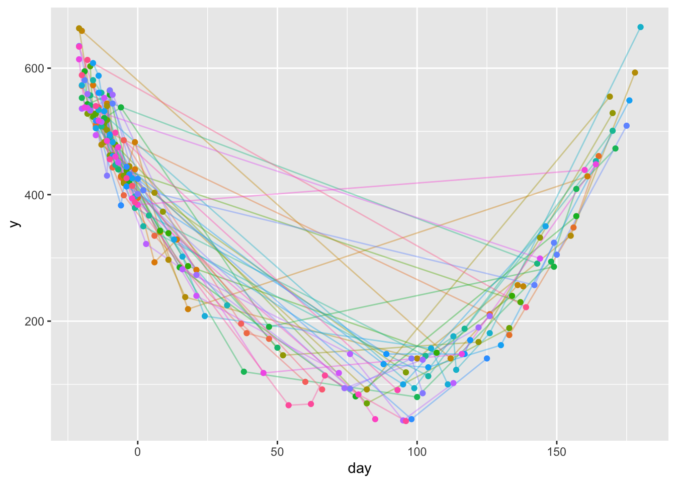
Simulate data, starting with simulating a random number npre of baseline measures from 1-5 and a possibly different random number npost of follow-up measurements from 1-5. Sample days without replacement so that measurements within subject are always on different days. The dataset has a subject-specific variable age that is not used in this analysis added to it. The overall mean time trend is quadratic in time.
set.seed(11)
n <- 40
w <- lapply(1 : n,
function(i) { npre <- sample(1:5, 1)
npost <- sample(1:5, 1)
day <- sort(c(sample(-21 : 0, npre),
sample(1 : 180, npost)))
age <- sample(40:80, 1)
y <- round(day + (day - 90)^2 / 20 + 30 * rnorm(npre + npost))
data.table(id=i, age, day, y=y)
} )
head(w)
u <- rbindlist(w)
u
# Show distribution of number of points per subject
with(u, table(table(id)))
u[, id := factor(id)]
ggplot(u, aes(x=day, y=y)) +
geom_line(aes(col=id, alpha=I(0.4)), data=u) +
geom_point(aes(col=id), data=u) +
guides(color='none')- 1
-
separately for integers 1, 2, 3, …, n runs a function on that integer with the function producing a
listthat is stored in an element of a largerlist; responseyis normal with mean being a quadratic function ofday - 2
-
argument
iis the subject number; for that subject simulate the number of observations then simulate data using that number - 3
-
stack all the little data tables into one tall data table
u - 4
-
ggplot2needs a variable mapped to thecoloraesthetic to be factor so it treats subjectidas categorical and doesn’t try to create a continuous color gradient
[[1]]
      id   age   day     y
   <int> <int> <int> <num>
1:     1    51    -6   427
2:     1    51    -5   486
3:     1    51    37   196
4:     1    51    60   104

[[2]]
      id   age   day     y
   <int> <int> <int> <num>
1:     2    42   -20   572
2:     2    42   -15   511
3:     2    42   -14   538
4:     2    42    -9   443
5:     2    42    -5   399
6:     2    42     6   335
7:     2    42    39   181
8:     2    42    47   172

[[3]]
      id   age   day     y
   <int> <int> <int> <num>
1:     3    66   -15   508
2:     3    66   126   211
3:     3    66   133   178
4:     3    66   156   348
5:     3    66   165   461

[[4]]
      id   age   day     y
   <int> <int> <int> <num>
1:     4    77   -16   573
2:     4    77    -6   429
3:     4    77    -1   440
4:     4    77     0   395
5:     4    77     6   293
6:     4    77    14   329
7:     4    77    21   281

[[5]]
      id   age   day     y
   <int> <int> <int> <num>
1:     5    42   -11   544
2:     5    42   -10   492
3:     5    42    -5   421
4:     5    42    -1   483
5:     5    42     8   341
6:     5    42    18   219
7:     5    42   161   429

[[6]]
      id   age   day     y
   <int> <int> <int> <num>
1:     6    58   -20   659
2:     6    58   112   141
3:     6    58   136   257
4:     6    58   138   255

        id   age   day     y
     <int> <int> <int> <num>
  1:     1    51    -6   427
  2:     1    51    -5   486
  3:     1    51    37   196
  4:     1    51    60   104
  5:     2    42   -20   572
 ---
218:    39    42   -20   589
219:    39    42   -18   613
220:    39    42   139   222
221:    40    48    -2   414
222:    40    48    66    92

2 3 4 5 6 7 8 9
4 3 4 9 5 9 3 3
For one subject write a function to compute all of the three summary measures for which the data needed are available. Don’t try to estimate the slope if some times are not at least 3 days apart. By returning a list the g function causes data.table to create three variables.
g <- function(x, y) {
j <- x <= 0 & ! is.na(y)
x <- x[j]; y <- y[j]
n <- length(x)
if(n == 0) return(list(y0 = NA_real_, ym8 = NA_real_, slope = NA_real_))
pre0 <- x >= -7
prem8 <- x < -7
list(y0 = if(any(pre0)) mean(y[pre0]) else NA_real_,
ym8 = if(any(prem8)) mean(y[prem8]) else NA_real_,
slope = if(length(x) > 1 && diff(range(x)) >= 3)
unname(coef(lsfit(x, y))[2]) else NA_real_)
}- 1
-
Analyze observations with non-missing
ythat are measured pre-intervention - 2
-
data.tablerequires all variables being created to have the same type for every observation; this includes the type ofNA - 3
-
range(x)computes a 2-vector with the min and maxx, anddiffsubtracts the min from the max. The&&and operator causesdiff(...)to not even be evaluated unless there are at least two points.lsfitis a simple function to fit a linear regression.coefextracts the vector of regression coefficients from the fit, and we keep the second coefficient, which is the slope. The slope carries an element name ofX(created bylsfit) which is removed byunname().
Check the function.
g(numeric(0), numeric(0))$y0
[1] NA
$ym8
[1] NA
$slope
[1] NAg(-10, 1)$y0
[1] NA
$ym8
[1] 1
$slope
[1] NAg(c(-10, -9), c(1, 2))$y0
[1] NA
$ym8
[1] 1.5
$slope
[1] NAg(c(-10, -3), c(1, 2))$y0
[1] 2
$ym8
[1] 1
$slope
[1] 0.1428571Now run the function separately on each subject. Then drop the pre-intervention records from the main data table u and merge the new baseline variables with the follow-up records.
base <- u[, g(day, y), by = .(id)]
head(base)
id y0 ym8 slope
<fctr> <num> <num> <num>
1: 1 456.5000 NA NA
2: 2 399.0000 516 -11.900901
3: 3 NA 508 NA
4: 4 421.3333 573 -10.073095
5: 5 452.0000 518 -6.131274
6: 6 NA 659 NAdim(u)[1] 222 4u <- u[day > 0] # Keep only post-intervention (follow-up) records
dim(u)[1] 115 4u <- Merge(base, u, id = ~ id) # Merge is in Hmisc Vars Obs Unique IDs IDs in #1 IDs not in #1
base 4 40 40 NA NA
u 4 115 40 40 0
Merged 7 115 40 40 0
Number of unique IDs in any data frame : 40
Number of unique IDs in all data frames: 40 uKey: <id>
id y0 ym8 slope age day y
<fctr> <num> <num> <num> <int> <int> <num>
1: 1 456.5 NA NA 51 37 196
2: 1 456.5 NA NA 51 60 104
3: 2 399.0 516 -11.90090 42 6 335
4: 2 399.0 516 -11.90090 42 39 181
5: 2 399.0 516 -11.90090 42 47 172
---
111: 38 407.0 498 -10.05983 57 62 69
112: 38 407.0 498 -10.05983 57 67 114
113: 38 407.0 498 -10.05983 57 96 42
114: 39 NA 601 NA 42 139 222
115: 40 414.0 NA NA 48 66 9213.5 Interpolation/Extrapolation to a Specific Time
Suppose that subjects have varying numbers of records, with some having only one measurement. Our goal is to summarize each subject with a single measurement targeted to estimate the subject’s response at 90 days. Our strategy is as follows:
- If the subject has a measurement at exactly 90 days, use it.
- If the subject has only one measurement, use that measurement to estimate that subject’s intercept (vertical shift), and use the time-response curve estimated from all subjects to extrapolate an estimate at 90 days.
- If the subject has two or more measurements, use the same approach but average all vertical shifts from the overall
loesscurve to adjust theloess“intercept” in estimatingyat the target time.
Use the data table u created above.
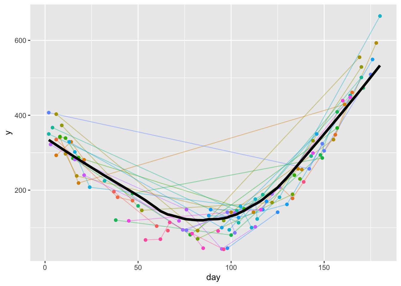
timeresp <- u[! is.na(day + y), approxfun(lowess(day, y))]
w <- data.table(day=1:180, y=timeresp(1:180))
ggplot(u, aes(x=day, y=y)) +
geom_line(aes(col=id, alpha=I(0.4)), data=u) +
geom_point(aes(col=id), data=u) +
geom_line(aes(x=day, y, size=I(1.5)), data=w) +
guides(color='none')- 1
-
lowessruns theloessnonparametric smoother and creates a list with vectorsxandy;approxfuntranslates this list into a function that linearly interpolates while doing the table look-up into thelowessresult.timerespis then a function to estimate the all-subjects-combined time-response curve.lowessdoesn’t handleNAs properly so we excluded points that are missing on either variable. - 2
- evaluates the whole time-response curve for day 1, 2, 3, …, 180
As done previously, we follow the good practice of perfecting a function that summarizes the data for one subject, then let data.table run that function separately by subject ID. The method adjusts the loess curve so that it perfectly fits one observed point or best fits all observed points on the average, then we use that adjusted curve to estimate the response at day 90. This is an empirical approach that trusts the raw data to provide the intercept, resulting in interpolated or extrapolated estimates that are as noisy as the real data. Function f also returns the number of days from 90 to the closest day used for estimation of day 90’s response.
f <- function(x, y, id=character(0), target=90) {
  j <- ! is.na(x + y)
    if(! any(j)) {
      cat('no non-missing x, y pairs for subject', id, '\n')
        return(list(day = target, distance=NA_real_, yest=NA_real_))
        }
  x <- x[! is.na(x)]; y <- y[! is.na(y)]
  distance <- abs(x - target)
  i        <- which(distance == 0)
  if(length(i)) return(list(day=target, distance=0., yest=mean(y[i])))
  # estimate mean y at observed x - mean loess at observed x to adjust
  z <- timeresp(c(target, x))
  list(day      = target,
       distance = min(distance),
       yest     = z[1] + mean(y) - mean(z[-1]) )
  }
Test the function under a variety of situations.
# n=1, y is on the loess curve so projected y at x=90 should be also
f(25, 253.0339)
$day
[1] 90
$distance
[1] 65
$yest
[1] 115.017timeresp(c(25, 90))[1] 260.3086 122.2918# n=1, x=90 exactly
f(90, 111.11)$day
[1] 90
$distance
[1] 0
$yest
[1] 111.11# n=3, two x=90
f(c(1, 2, 90, 90), c(37, 3, 33, 34))$day
[1] 90
$distance
[1] 0
$yest
[1] 33.5# n=1, not on loess curve
f(25, timeresp(25) - 100)$day
[1] 90
$distance
[1] 65
$yest
[1] 22.29177timeresp(90) - 100[1] 22.29177# n=2, interpolate to 90 guided by loess
f(c(80, 100), c(100, 200))$day
[1] 90
$distance
[1] 10
$yest
[1] 146.486# n=2, extrapolate to 90
f(c(70, 80), c(100, 200))$day
[1] 90
$distance
[1] 10
$yest
[1] 146.9803Now apply the function to each subject. Add the new points to the original plot. Keep the age variable in the one subject per record data table z.
z <- u[, c(list(age=age), f(day, y, id)), by=id]   # just use u[, f(day, y, id), ...] if don't need age
# Show distribution of distance between 90 and closest observed day
z[, table(distance)]
distance
1 2 3 5 6 8 9 10 12 13 14 15 17 18 22 24 26 30 32 36 40 43 47 49 52 53
3 4 1 10 5 10 5 10 8 4 3 4 5 2 3 1 3 2 5 4 1 5 1 1 5 1
54 58 69 70 71
1 1 3 1 3 ggplot(u, aes(x=day, y=y)) +
geom_line(aes(col=id), data=u) +
geom_point(aes(col=id), data=u) +
geom_line(aes(x=day, y, size=I(1.5)), data=w) +
geom_point(aes(x=day, y=yest, col=id, shape=I('x'), size=I(3)), data=z) +
guides(color='none')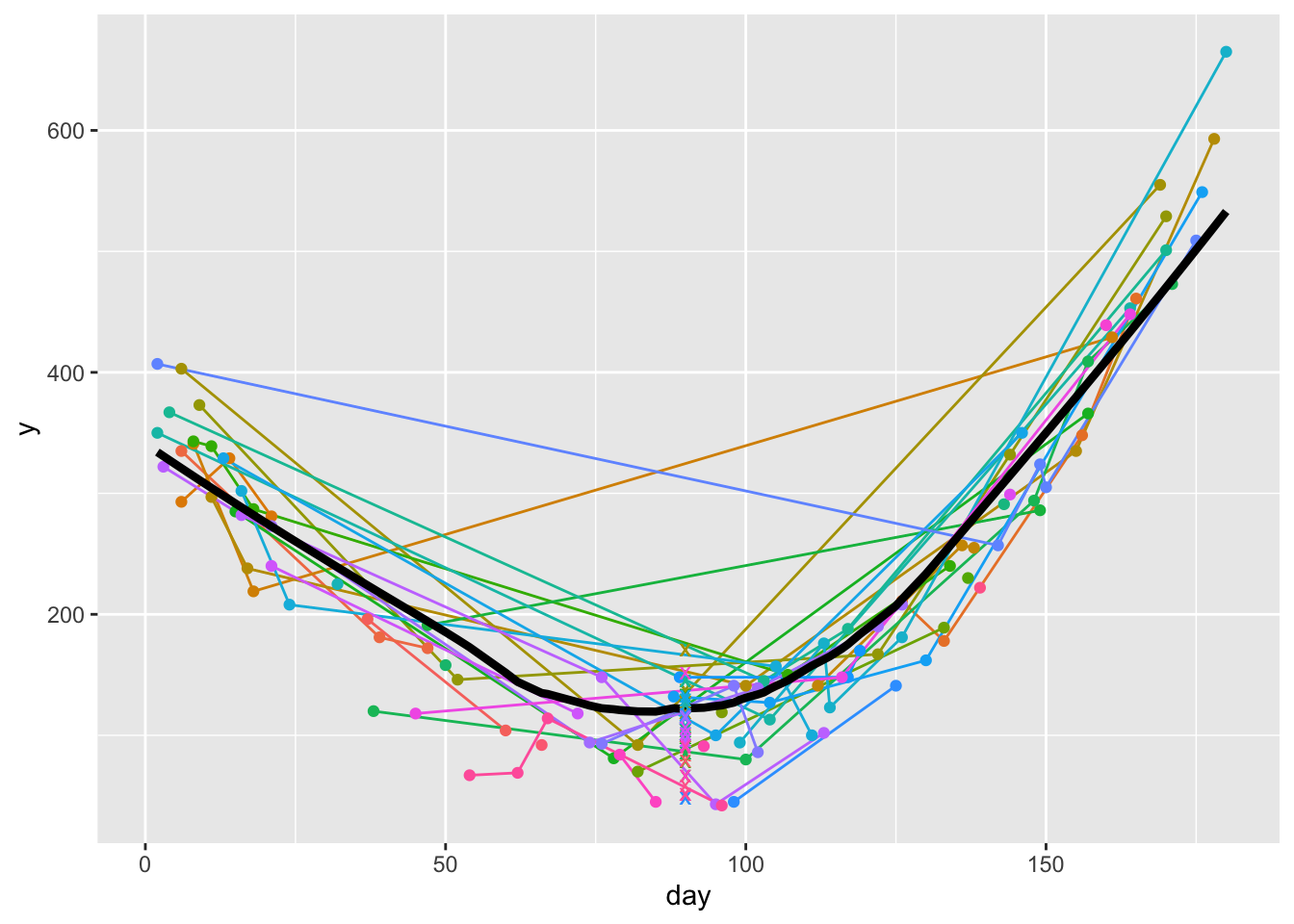
13.6 Linear Interpolation to a Vector of Times
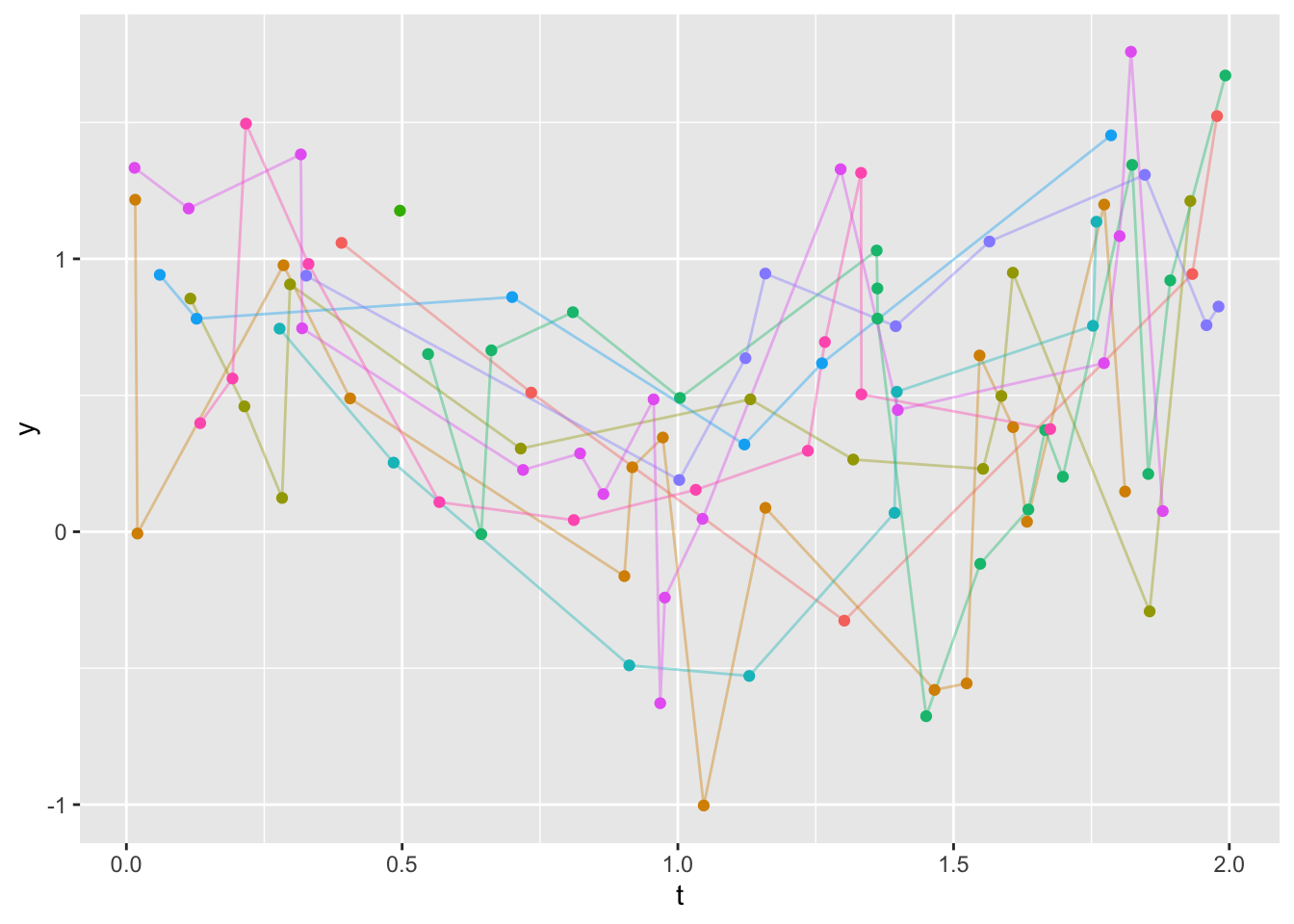
Suppose that 10 subjects have varying numbers of records, corresponding to assessment times t ranging from 0 to 2 years. We want to estimate the values of variable y over a regular sequence of values 0.25 years apart, for all subjects having at least two records at distinct times. Use linear interpolation, or linear extrapolation if one of the target times is outside the range of a subject’s data. It is advisable to specify the time sequence as consisting of points interior to [0, 2] so that the estimates at the end have a good chance to be symmetrically interpolated/extrapolated. For any value of t in the grid, set the calculated interpolated/extrapolated value to NA if there is no measurement within 0.25 years of t.
Create the test dataset and a function to do the calculations on a single subject.
set.seed(15)
n <- 10
w <- lapply(1 : n,
function(i) { m <- sample(1 : 20, 1)
t <- sort(runif(m, 0, 2))
y <- abs(t - 1) + 0.5 * rnorm(m)
data.table(id=as.character(i), t, y)})
u <- rbindlist(w)
# Show distribution of number of points per subject
with(u, table(table(id)))
ggplot(u, aes(x=t, y=y)) +
geom_line(aes(col=id, alpha=I(0.4)), data=u) +
geom_point(aes(col=id), data=u) +
guides(color='none')- 1
- Number of assessments for a subject is a random number between 1 and 20
- 2
- Uniformly distributed assessment times in ascending order
- 3
- True responses have means that are V-shaped in time
- 4
-
Setting
idto a character variable will keepggplot2from trying to treatidas a continuous variable - 5
- Using a transparency of 0.4 makes it easier to read spaghetti plots
- 6
-
Prevent
ggplot2from creating a legend forid
 1  5  6  8  9 12 16 17
 1  1  1  1  1  2  1  2
# Set target times to regularize to
times <- seq(0.25, 1.75, by=0.25)
g <- function(t, y) {
i <- ! is.na(y)
if(any(! i)) {
t <- t[i]
y <- y[i]
}
if(uniqueN(t) < 2) return(list(t=times, y=rep(NA_real_, length(times))))
z <- approxExtrap(t, y, xout=times)$y
# For each target time compute the number of measurements within 0.25
# years of the target
nclose <- sapply(times, function(x) sum(abs(t - x) <= 0.25))
z[nclose < 1] <- NA_real_
list(t=times, y=z)
}- 1
-
gis a function of two vectors (all values for one subject) that returns alist, which makesdata.tableplace the output into two variables with names given inlist()(t and y) - 2
-
uniqueNis indata.tableand computes the number of distinct values of its argument. Remember that when you needNAplaceholders in building adata.tableyou need to declare the storage mode for theNA. Hererealmeans double precision floating point (16 digits of precision, the standard R non-integer numeric). - 3
-
approxExtrapis in theHmiscpackage. It extends the built-in Rapproxfunction to do linear extrapolation.
Test the function.
g(1, 1)$t
[1] 0.25 0.50 0.75 1.00 1.25 1.50 1.75
$y
[1] NA NA NA NA NA NA NAg(1:2, 11:12)$t
[1] 0.25 0.50 0.75 1.00 1.25 1.50 1.75
$y
[1] NA NA 10.75 11.00 11.25 NA 11.75Create a data table with the new variables, and plot the derived estimates along with the raw data. X’s are regularized y-values. X’s that are not touching lines represent extrapolations, and those on lines are interpolations.
z <- u[, g(t, y), by=id]
ggplot(u, aes(x=t, y=y)) +
  geom_line(aes(col=id), data=u) +
  geom_point(aes(col=id), data=u) +
  geom_point(aes(x=t, y=y, col=id, shape=I('x'), size=I(4)), data=z) +
  guides(color='none')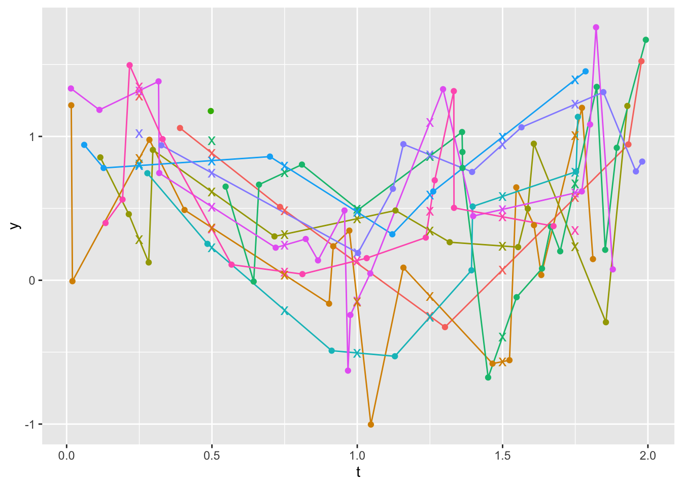
Look at raw data for the two Xs on the plot that are not touching lines at t=0.25 (id=7) and 0.5 (id=4). For id=4 the X marks an extrapolation to the left of a steep drop over the first two points. For id=7 there is also extrapolation to the left.
u[id %in% c(4,7)] id t y
<char> <num> <num>
1: 4 0.5470506 0.651103767
2: 4 0.6435926 -0.008838958
3: 4 0.6618349 0.664723930
4: 4 0.8096265 0.804353411
5: 4 1.0037501 0.490364169
6: 4 1.3605564 1.030634292
7: 4 1.3618222 0.891685917
8: 4 1.3620511 0.780965231
9: 4 1.4502774 -0.676070873
10: 4 1.5483572 -0.117616105
11: 4 1.6356089 0.081489276
12: 4 1.6660358 0.372573268
13: 4 1.6981980 0.201474172
14: 4 1.8238231 1.344406932
15: 4 1.8530522 0.211624201
16: 4 1.8928997 0.920978736
17: 4 1.9928758 1.671926932
18: 7 0.3260752 0.938380892
19: 7 1.0025397 0.189611500
20: 7 1.1225979 0.635890259
21: 7 1.1586452 0.946132952
22: 7 1.3950600 0.753206290
23: 7 1.5650036 1.063503814
24: 7 1.8467943 1.307851168
25: 7 1.9586770 0.756841672
26: 7 1.9804584 0.825144644
id t y
<char> <num> <num>Let’s summarize the regularized data by computing the interpolated y at t=1, Gini’s mean difference, and mean absolute consecutive y difference for each subject. Also compute the number of non-missing regularized values.
g <- function(y) {
n <- sum(! is.na(y))
if(n < 2) return(list(n=n, y1=NA_real_, gmd=NA_real_, consec=NA_real_))
list(n = n,
y1 = y[abs(times - 1.) < 0.001],
gmd = GiniMd(y, na.rm=TRUE),
consec = mean(abs(y - Lag(y)), na.rm=TRUE))
}
g(c(1, 2, NA, 5, 8, 9, 10))
w <- z[, g(y), by=id]
w- 1
-
Checking against integers such as times = 1 will not have a problem with code such as
y[times == 1]but to work in general when values being checked for equality may not be exactly represented in base 2 it’s best to allow for a tolerance such as 0.001. - 2
-
Lagis in theHmiscpackage; by default it shifts the y vector back one observation
$n
[1] 6

$y1
[1] 5

$gmd
[1] 4.6

$consec
[1] 1.5

        id     n         y1       gmd    consec
    <char> <int>      <num>     <num>     <num>
 1:      1     6         NA 0.6785255 0.4052871
 2:      2     7  0.4282241 0.1502275 0.1544205
 3:      3     0         NA        NA        NA
 4:      4     6  0.4964298 0.5336070 0.6330032
 5:      5     7 -0.5053917 0.6432752 0.4290084
 6:      6     7  0.4744770 0.3438133 0.2189778
 7:      7     6  0.1924227 0.4040584 0.3270544
 8:      8     7 -0.1416566 0.5904388 0.5696528
 9:      9     7  0.1374026 0.4416730 0.3067097
10:     10     7 -0.1504149 0.6846669 0.5107083
13.7 Overlap Joins and Non-equi Merges
Section 12.2 covered simple inexact matching/merging. Now consider more complex tasks.
The foverlaps function in data.table provides an amazingly fast way to do complex overlap joins. Our first example is modified from an example in the help file for foverlaps. An annotation column is added to describe what happened.
d1 <- data.table(w     =.q(a, a, b, b, b),
                 start = c( 5, 10, 1, 25, 50),
                 end   = c(11, 20, 4, 52, 60))
d2 <- data.table(w     =.q(a, a, b),
                 start = c(1, 15,  1),
                 end   = c(4, 18, 55),
                 name  = .q(dog, cat, giraffe),
                 key   = .q(w, start, end))
f <- foverlaps(d1, d2, type="any")
ann <- c('no a overlap with d1 5-11 & d2 interval',
         'a 10-20 overlaps with a 16-18',
         'b 1-4 overlaps with b 1-55',
         'b 25-62 overlaps with b 1-55',
         'b 50-60 overlaps with b 1-55')
f[, annotation := ann]
f
w start end name i.start i.end
<char> <num> <num> <char> <num> <num>
1: a NA NA <NA> 5 11
2: a 15 18 cat 10 20
3: b 1 55 giraffe 1 4
4: b 1 55 giraffe 25 52
5: b 1 55 giraffe 50 60
annotation
<char>
1: no a overlap with d1 5-11 & d2 interval
2: a 10-20 overlaps with a 16-18
3: b 1-4 overlaps with b 1-55
4: b 25-62 overlaps with b 1-55
5: b 50-60 overlaps with b 1-55# Don't include record for non-match
foverlaps(d1, d2, type='any', nomatch=NULL) w start end name i.start i.end
<char> <num> <num> <char> <num> <num>
1: a 15 18 cat 10 20
2: b 1 55 giraffe 1 4
3: b 1 55 giraffe 25 52
4: b 1 55 giraffe 50 60# Require the d1 interval to be within the d2 interval
foverlaps(d1, d2, type="within") w start end name i.start i.end
<char> <num> <num> <char> <num> <num>
1: a NA NA <NA> 5 11
2: a NA NA <NA> 10 20
3: b 1 55 giraffe 1 4
4: b 1 55 giraffe 25 52
5: b NA NA <NA> 50 60# Require the intervals to have the same starting point
foverlaps(d1, d2, type="start") w start end name i.start i.end
<char> <num> <num> <char> <num> <num>
1: a NA NA <NA> 5 11
2: a NA NA <NA> 10 20
3: b 1 55 giraffe 1 4
4: b NA NA <NA> 25 52
5: b NA NA <NA> 50 60Now consider an example where there is an “events” dataset e with 0 or more rows per subject containing start (s) and end (e) times and a measurement x representing a daily dose of something given to the subject from s to e. The base dataset b has one record per subject with times c and d. Compute the total dose of drug received between c and d for the subject. This is done by finding all records in e for the subject such that the interval [c,d] has any overlap with the interval [s,e]. For each match compute the number of days in the interval [s,e] that are also in [c,d]. This is given by min(e,d) + 1 - max(c,s). Multiply this duration by x to get the total dose given in [c,d]. For multiple records with intervals touching [c,d] add these products.
base   <- data.table(id    = .q(a,b,c), low=10, hi=20)
events <- data.table(id    = .q(a,b,b,b,k),
                     start = c( 8,  7, 12, 19, 99),
                     end   = c( 9,  8, 14, 88, 99),
                     dose  = c(13, 17, 19, 23, 29))
setkey(base,   id, low,   hi)
setkey(events, id, start, end)
w <- foverlaps(base, events,
               by.x = .q(id, low,   hi),
               by.y = .q(id, start, end ),
               type = 'any', mult='all', nomatch=NA)

w[, elapsed := pmin(end, hi) + 1 - pmax(start, low)]
w[, .(total.dose = sum(dose * elapsed, na.rm=TRUE)), by=id]
Key: <id>
id total.dose
<char> <num>
1: a 0
2: b 103
3: c 0Similar things are can be done with non-equi merges. For those you can require exact subject matches but allow inexact matches on other variables. The following example is modified from here. A medication dataset holds the start and end dates for a patient being on a treatment, and a second dataset visit has one record per subject ID per doctor visit. For each visit look up the drug in effect if there was one.
medication <-
  data.table(ID         = c( 1, 1, 2, 3, 3),
             medication = .q(a, b, a, a, b),
             start      = as.Date(c("2003-03-25","2006-04-27","2008-12-05",
                                    "2004-01-03","2005-09-18")),
             stop       = as.Date(c("2006-04-02","2012-02-03","2011-05-03",
                                    "2005-06-30","2010-07-12")),
             key        = 'ID')
medication
Key: <ID>
ID medication start stop
<num> <char> <Date> <Date>
1: 1 a 2003-03-25 2006-04-02
2: 1 b 2006-04-27 2012-02-03
3: 2 a 2008-12-05 2011-05-03
4: 3 a 2004-01-03 2005-06-30
5: 3 b 2005-09-18 2010-07-12set.seed(123)
visit <- data.table(
ID = rep(1:3, 4),
date = sample(seq(as.Date('2003-01-01'), as.Date('2013-01-01'), 1), 12),
sbp = round(rnorm(12, 120, 15)),
key = c('ID', 'date'))
visitKey: <ID, date>
ID date sbp
<int> <Date> <num>
1: 1 2004-06-09 113
2: 1 2006-06-06 147
3: 1 2008-01-16 126
4: 1 2009-09-28 127
5: 2 2003-07-14 138
6: 2 2006-02-15 122
7: 2 2006-06-21 127
8: 2 2009-11-15 101
9: 3 2005-11-03 91
10: 3 2009-02-04 110
11: 3 2011-03-05 125
12: 3 2012-03-24 112# Variables named in inequalities need to have variables in
# medication listed first
m <- medication[visit, on = .(ID, start <= date, stop > date)]
m ID medication start stop sbp
<int> <char> <Date> <Date> <num>
1: 1 a 2004-06-09 2004-06-09 113
2: 1 b 2006-06-06 2006-06-06 147
3: 1 b 2008-01-16 2008-01-16 126
4: 1 b 2009-09-28 2009-09-28 127
5: 2 <NA> 2003-07-14 2003-07-14 138
6: 2 <NA> 2006-02-15 2006-02-15 122
7: 2 <NA> 2006-06-21 2006-06-21 127
8: 2 a 2009-11-15 2009-11-15 101
9: 3 b 2005-11-03 2005-11-03 91
10: 3 b 2009-02-04 2009-02-04 110
11: 3 <NA> 2011-03-05 2011-03-05 125
12: 3 <NA> 2012-03-24 2012-03-24 112# start and stop dates are replaced with actual date of visit
# drop one of them and rename the other
m[, stop := NULL]
setnames(m, 'start', 'date')
m ID medication date sbp
<int> <char> <Date> <num>
1: 1 a 2004-06-09 113
2: 1 b 2006-06-06 147
3: 1 b 2008-01-16 126
4: 1 b 2009-09-28 127
5: 2 <NA> 2003-07-14 138
6: 2 <NA> 2006-02-15 122
7: 2 <NA> 2006-06-21 127
8: 2 a 2009-11-15 101
9: 3 b 2005-11-03 91
10: 3 b 2009-02-04 110
11: 3 <NA> 2011-03-05 125
12: 3 <NA> 2012-03-24 11213.8 Using Large Language Models as data.table Coding Assistants
Large language models are now useful for assisting in coding for fairly complex tasks, if the user is willing to throughly test the generated code. This makes powerful syntax and fast execution time of data.table even more available to users. The following query was given to ChatGPT on 2025-08-21.
Using the R language and only using the R
data.tablepackage and base R code, write code to solve the following problem. Consider a data.table namedAwith variablesid, sex, yand a data.table namedBwith variablesid, y, z.Ahas one record per distinctidandBhas possibly multiple records perid. JoinAandBbyid, keeping the record inBthat is closest on theyvalue to the value ofyinA. If there is no observation within 5 units ofyforsex=='male'or within 7 units ofyforsex=='female', set the value ofyin the joined data table toNA.
The reply from ChatGPT and the ensuing dialog follow. The only changes in the text were to actually execute the generated R code here, to remove superfluous print() around objects to be printed, and to use a special font for R object names and expressions in sentences.
Got it 👍 — this is a “closest match join with tolerance” problem. We want:
- For each
A[id], find the row inB[id]withyclosest toA$y.- Tolerance depends on
sex.- If no
B$ywithin tolerance, returnNAfor they(andz) fromB.
Here’s a pure data.table + base R solution:
A <- data.table(id = c(1, 2, 3, 4),
                sex = c("male", "female", "male", "female"),
                y   = c(10, 20, 30, 40))

B <- data.table(id = c(1,1,1,2,2,3,3,4),
                y  = c(12, 17, 25, 15, 30, 28, 40, 100),
                z  = letters[1:8])

setkey(A, id)
setkey(B, id)

result <- B[A, allow.cartesian=TRUE][
  , diff := abs(i.y - y), by=.(id, i.y, sex)][
  , .SD[which.min(diff)], by=.(id, i.y, sex)][
  , tol := ifelse(sex=="male", 5, 7)][
  , `:=`(
    y = ifelse(diff <= tol, y, NA_real_),
    z = ifelse(diff <= tol, z, NA_character_)
  )][
  , .(id, sex, yA = i.y, yB = y, z)]

result
id sex yA yB z
<num> <char> <num> <num> <char>
1: 1 male 10 12 a
2: 2 female 20 15 d
3: 3 male 30 28 f
4: 4 female 40 NA <NA>Explanation of steps:
B[A, allow.cartesian=TRUE]→ join allBrows for eachA$id.- Compute
diff = |A$y - B$y|for each candidate.which.min(diff)→ select closestBrow for each (id, A$y, sex).- Define tolerance by
sex(5 for male, 7 for female`).- If
diff > tol, replaceyandzfromBwithNA.
Write a function named
gthat does as many of the calculations as possible outside ofdata.tablesyntax, and use this function withindata.tablesyntax to arrive at the same answer as you obtained already.
Great request 👍 — you want to push the “heavy lifting” (the min-diff calculation + tolerance check) into a base R function and then just use that inside
data.tablegrouping. That way thedata.tablecode is lean.Here’s a way to do it:
# Function to select the best match given one row of A and all rows of B for that id
g <- function(yA, sex, yB, zB) {
  # tolerance by sex
  tol <- if (sex == "male") 5 else 7

  # if no candidates, return NA
  if (length(yB) == 0) return(list(yB = NA_real_, zB = NA_character_))

  # find closest yB
  diffs <- abs(yA - yB)
  j <- which.min(diffs)

  if (diffs[j] <= tol) {
    return(list(yB = yB[j], zB = zB[j]))
  } else {
    return(list(yB = NA_real_, zB = NA_character_))
  }
}

# Apply inside data.table syntax
setkey(A, id)
setkey(B, id)

result <- B[A, allow.cartesian=TRUE][
  , g(i.y, sex[1L], y, z), by=.(id, sex, i.y)]

# Clean names
setnames(result, c("id","sex","yA","yB","z"))

result
id sex yA yB z
<num> <char> <num> <num> <char>
1: 1 male 10 12 a
2: 2 female 20 15 d
3: 3 male 30 28 f
4: 4 female 40 NA <NA>How it works
g()is pure base R. It:
- Decides the tolerance.
- Finds the closest
yB.- Returns either the
yB/zBpair orNA.- Inside the join, we just call
g()grouped by (id, sex, i.y).- The output matches the earlier solution.
I don’t understand the subscripting of
sexwhen computing the result.
Ah good eye 👀 — the
sex[1L]part ing(i.y, sex[1L], y, z)deserves an explanation.Why
sex[1L]?
- After the join
B[A, allow.cartesian=TRUE], each row ofA(with itssexandy, stored asi.y) is paired with all rows ofBthat share the sameid.- So within each group (
id, sex, i.y),sexis repeated many times (once for eachBrow).Example: suppose
A: id=1, sex="male", y=10B: id=1has 3 rowsThen the join produces 3 rows, and each of those rows carries
sex="male".So inside the group,
sexis a vector likec("male","male","male").
- But we only need one value of sex to send to
g()— it’s the same across all rows in the group.- So we just take the first element,
sex[1L]. (The1Lis an integer literal, a habit indata.tableto be explicit and efficient.)
What would happen of
allow.cartesian=TRUEwere not included?
This goes right to the heart of why
allow.cartesian=TRUEis sometimes needed withdata.table.Without
allow.cartesian=TRUEB[A]# same asB[A, allow.cartesian=FALSE]
- By default, data.table does not allow one-to-many or many-to-many joins unless you explicitly tell it it’s OK.
- If
Ahasid=1once, andBhas id=1 three times, the join would need to return 3 rows for that one row ofA(a Cartesian product).- That’s exactly the situation in your problem: each row in
Ajoins to potentially multiple rows inB.So if you left out
allow.cartesian=TRUE, you’d get an error like:Error in
B[A]: join results in more than one match per row of ‘i’; please useallow.cartesian=TRUEto proceedWith
allow.cartesian=TRUE
- You explicitly acknowledge: “Yes, I know this join may expand rows, that’s what I want.”
- Then
Arows are duplicated for each matching row inB.- That expansion is exactly what we need before we calculate distances and pick the closest
y.✅ In short:
Without it → error if one row in
Amatches multiple inB. With it → allowed expansion (the Cartesian join), which we need for the “closest match” problem.
But I frequently use
data.tableto do one to many joins (Ahas one record peridandBhas one or more records perid) and have gotten the multiple matches retained without specifyingallow.cartesian=TRUE.
Excellent point — and you’re right 👍. Let’s unpack what’s going on, because the difference is subtle and can be confusing.
Case 1:
B[A](Aon theiside)When you do:
B[A]
Ais on theiside of the join.data.tablesays: “For each row ofA, pull matching rows fromB.”- If one row in
Amatches many rows inB, those matches are returned by default — noallow.cartesianneeded.- That’s the normal one-to-many join you’re used to.
✅ So this is why your experience is that you don’t need a
llow.cartesian=TRUECase 2: Both sides can repeat → Cartesian explosion
allow.cartesian=TRUEonly becomes necessary when the join can multiply rows in both directions (i.e. many-to-many).For example:
A <- data.table(id=1:2, x=1:2)
B <- data.table(id=c(1,1), y=1:2)Both have duplicate ids (
Ahas 1 row withid=1,Bhas 2 rows withid=1)B[A]This works fine (no error):
id y x
1: 1 1 1
2: 1 2 1
3: 2 NA 2But if both
AandBhave multiple rows perid, the join could create Cartesian products. That’s whereallow.cartesiankicks in:
A <- data.table(id=c(1,1), x=1:2)# 2 rows with id=1
B <- data.table(id=c(1,1), y=1:2)# 2 rows with id=1
B[A]Error: Error in
B[A]: join results in more than one match per row ofi; please useallow.cartesian=TRUEto proceedBecause now one row in A can match multiple in
B, andAitself has duplicates — so the join multiplies. That’s a true Cartesian join.Back to your problem
- In your setup,
Ahas exactly one row perid.Bcan have many rows perid.- That’s just a one-to-many join → no need for
allow.cartesian=TRUE.I included it earlier as a “safe guard” because in testing toy examples, sometimes
Aaccidentally has duplicates, and then you hit the error. But if you knowAreally is one row perid, you can safely omit it.