24  Bacteremia: Case Study in Nonlinear Data Reduction with Imputation

Data

• Study of 14,691 patients to analyze risk of bacteremia on the basis of many highly standardized blood analysis parameters
• Vienna General Hospital 2006-2010
• Ratzinger et al
• Data modified for public use by Heinze and available for easy use in R at hbiostat.org/data

Methods Illustrated

• Multiple imputation
• Variable clustering with pairwise deletion of NAs
• Stacking of multiply-imputed datasets so that single analyses can be done (Morris et al. (2015))
• Optimum unsupervised nonlinear transformations
• Redundancy analysis
• Sparse principal components
• High-level statistical reporting functions in the qreport package (dataOverview, missChk, vClus)

The optimum nonlinear transformations are determined form the transace function in the Hmisc package, which uses the ACE algorithm. Nonlinear transformations, redundancy analysis, and sparse PCs are all done on a tall stacked multiply-imputed dataset.

24.1 Descriptive Statistics

Click on the tabs to see the different kinds of variables. Hover over spike histograms to see frequencies and details about binning.

getHdata(bacteremia)
d <- bacteremia
# Load javascript dependencies for interactive spike histograms
sparkline::sparkline(0)

maketabs(print(describe(d), 'both'),
         cwidth='column-screen-inset-shaded')

Continuous

d Descriptives
51 Continous Variables of 53 Variables, 14691 Observations
Variable	Label	Units	n	Missing	Distinct	Info	Mean	Gini |Δ|		Quantiles .05 .10 .25 .50 .75 .90 .95
id	Patient Identification		14691	0	14691	1.000	29353	20965		2206 4834 13586 28755 44670 55598 59070
age	Patient Age	years	14691	0	85	1.000	56.17	20.78		24 29 43 58 70 79 84
mcv	Mean corpuscular volume	pg	14649	42	506	1.000	88.35	6.992		78.2 81.1 84.7 88.3 92.0 95.9 99.0
hgb	Haemoglobin	G/L	14650	41	157	1.000	11.57	2.558		8.2 8.8 9.9 11.4 13.2 14.6 15.4
hct	Haematocrit	%	14649	42	404	1.000	34.48	7.316		24.6 26.4 29.8 34.3 39.1 42.9 44.8
plt	Blood platelets	G/L	14649	42	718	1.000	220	130.1		50 81 140 204 277 369 445
mch	Mean corpuscular hemoglobin	fl	14649	42	232	1.000	29.58	2.693		25.3 26.7 28.4 29.7 31.0 32.4 33.4
mchc	Mean corpuscular hemoglobin concentration	g/dl	14649	42	124	0.999	33.47	1.546		31.1 31.7 32.6 33.5 34.4 35.2 35.6
rdw	Red blood cell distribution width	%	14635	56	173	1.000	15	2.385		12.4 12.7 13.4 14.5 16.0 18.0 19.5
mpv	Mean platelet volume	fl	13989	702	71	0.999	10.38	1.132		8.9 9.2 9.7 10.3 11.0 11.7 12.2
lym	Lymphocytes	G/L	14429	262	114	0.998	1.366	1.162		0.2 0.4 0.7 1.0 1.6 2.1 2.6
mono	Monocytes	G/L	14445	246	67	0.996	0.8527	0.5965		0.1 0.3 0.5 0.8 1.1 1.5 1.8
eos	Eosinophils	G/L	14556	135	36	0.867	0.1148	0.1585		0.0 0.0 0.0 0.1 0.1 0.3 0.4
baso	Basophils	G/L	14545	146	18	0.337	0.01725	0.03111		0.0 0.0 0.0 0.0 0.0 0.1 0.1
nt	Normotest	%	12224	2467	149	1.000	83.22	30.56		35 48 67 83 101 118 128
aptt	Activated partial thromboplastin time	sec	12142	2549	631	1.000	40.06	9.533		30.1 31.4 34.1 37.7 42.7 49.9 56.6
fib	Fibrinogen	mg/dl	12124	2567	1084	1.000	547.4	231		247 301 397 529 674 816 892
sodium	Sodium	mmol/L	13409	1282	58	0.994	137.2	5.034		129 132 135 137 140 142 144
potass	Potassium	mmol/L	12683	2008	408	1.000	4.003	0.6004		3.20 3.39 3.66 3.95 4.29 4.67 4.92
ca	Calcium	mmol/L	13415	1276	185	1.000	2.214	0.2213		1.89 1.96 2.09 2.22 2.35 2.45 2.51
phos	Phosphate	mmol/L	13449	1242	306	1.000	1.048	0.3993		0.55 0.64 0.81 0.99 1.20 1.47 1.74
mg	Magnesium	mmol/L	12822	1869	146	0.999	0.8136	0.1609		0.59 0.64 0.72 0.81 0.89 0.98 1.06
crea	Creatinine	mg/dl	14532	159	674	1.000	1.329	0.8518		0.620 0.690 0.810 1.000 1.350 2.160 3.144
bun	Blood urea nitrogen	mg/dl	14519	172	947	1.000	22.66	16.92		7.1 8.6 11.6 16.6 26.9 44.8 60.8
hs	Uric acid	mg/dl	11630	3061	169	1.000	5.413	2.625		2.2 2.7 3.7 5.0 6.6 8.5 10.0
gbil	Bilirubin	mg/dl	13250	1441	885	1.000	1.406	1.477		0.33 0.39 0.53 0.77 1.23 2.34 3.96
tp	Total protein	G/L	13108	1583	649	1.000	64.9	12.97		45.20 49.47 56.90 65.70 73.30 78.80 82.00
alb	Albumin	G/L	13015	1676	401	1.000	33.42	8.513		21.3 23.6 27.9 33.6 39.1 43.2 45.2
amy	Amylase	U/L	10778	3913	488	1.000	90.83	100.5		18 23 33 49 76 125 187
pamy	Pancreas amylase	U/L	7577	7114	280	0.999	41.66	47.28		7 9 14 22 36 64 97
lip	Lipases	U/L	10992	3699	444	1.000	63.82	89.88		6 8 14 23 40 79 135
che	Cholinesterase	kU/L	12244	2447	997	1.000	4.79	2.378		1.70 2.17 3.15 4.60 6.22 7.65 8.49
ap	Alkaline phosphatase	U/L	13291	1400	672	1.000	118.8	91.51		42 49 63 84 123 206 302
asat	Aspartate transaminase	U/L	13537	1154	650	1.000	86.9	115.6		15 17 22 31 56 121 218
alat	Alanin transaminase	U/L	13704	987	578	1.000	67.66	90.07		9 11 16 26 48 101 175
ggt	Gamma-glutamyl transpeptidase	G/L	13429	1262	858	1.000	115.1	141.3		13.0 16.0 25.0 49.0 117.0 262.2 429.0
ldh	Lactate dehydrogenase	U/L	12977	1714	1137	1.000	331.2	240.9		136 152 187 239 332 508 724
ck	Creatine kinase	U/L	12611	2080	1506	1.000	385	615.4		18 25 42 80 184 577 1155
glu	Glucose	mg/dl	10499	4192	389	1.000	126.4	48.3		78 85 97 113 138 177 216
trig	Triclyceride	mg/dl	9630	5061	538	1.000	141.7	90.33		54 64 83 115 165 241 307
chol	Cholesterol	mg/dl	9646	5045	339	1.000	150.8	59.23		74 89 113 145 182 219 243
crp	C-reactive protein	mg/dl	14536	155	3328	1.000	10.92	10.39		0.29 0.77 2.87 8.57 16.45 24.49 29.61
basor	Basophil ratio	%	13959	732	419	0.322	0.145	0.2679		0.0000 0.0000 0.0000 0.0000 0.0000 0.5501 1.0526
eosr	Eosinophil ratio	%	13959	732	927	0.891	1.297	1.825		0.0000 0.0000 0.0000 0.5882 1.7857 3.4900 5.0000
lymr	Lymphocyte ratio	% (mg/dl)	13959	732	3121	1.000	14.61	11.87		2.752 4.000 6.757 11.340 18.182 27.869 36.620
monor	Monocyte ratio	%	13959	732	2334	1.000	8.793	5.4		2.000 3.390 5.634 8.000 10.870 14.141 17.021
neu	Neutrophiles	G/L	13963	728	374	1.000	8.367	5.776		1.60 2.70 4.60 7.30 10.80 15.08 18.40
neur	Neutrophile ratio	%	13959	732	3850	1.000	75.15	15.6		47.42 57.88 69.23 78.33 85.32 90.13 92.63
pdw	Platelet distribution width	%	13589	1102	167	1.000	12.29	2.375		9.3 9.8 10.8 12.0 13.4 15.1 16.4
rbc	Red blood count	T/L	14230	461	65	0.999	3.936	0.8772		2.7 2.9 3.4 3.9 4.5 4.9 5.2
wbc	White blood count	G/L	14229	462	2710	1.000	11.23	7.602		2.66 4.26 6.63 9.60 13.53 18.22 22.27

Categorical

d Descriptives
2 Categorical Variables of 53 Variables, 14691 Observations
Variable	Label	n	Missing	Distinct	Info	Sum	Mean	Gini |Δ|
sex	Patient sex	14691	0	2
bacteremia	Bacteremia present by blood culture	14691	0	2	0.222	1180	0.08032	0.1477

dataOverview(d, id = ~ id)

d has 14691 observations (3979 complete) and 53 variables (4 complete) There are 14691 unique values of ID variable id in d

[ 0, 42) 42 [ 56, 159) [ 159, 461) [ 461, 987) [ 987,1262) [1262,1583) [1583,2008) [2008,2567) [2567,4192) [4192,7114]

Intervals of frequencies of NAs used for color-coding plots

Continuous

Plot of the degree of symmetry of the distribution of a variable (value of 1.0 is most symmetric) vs. the number of distinct values of the variable. Hover over a point to see the variable name and detailed characteristics.

Discrete

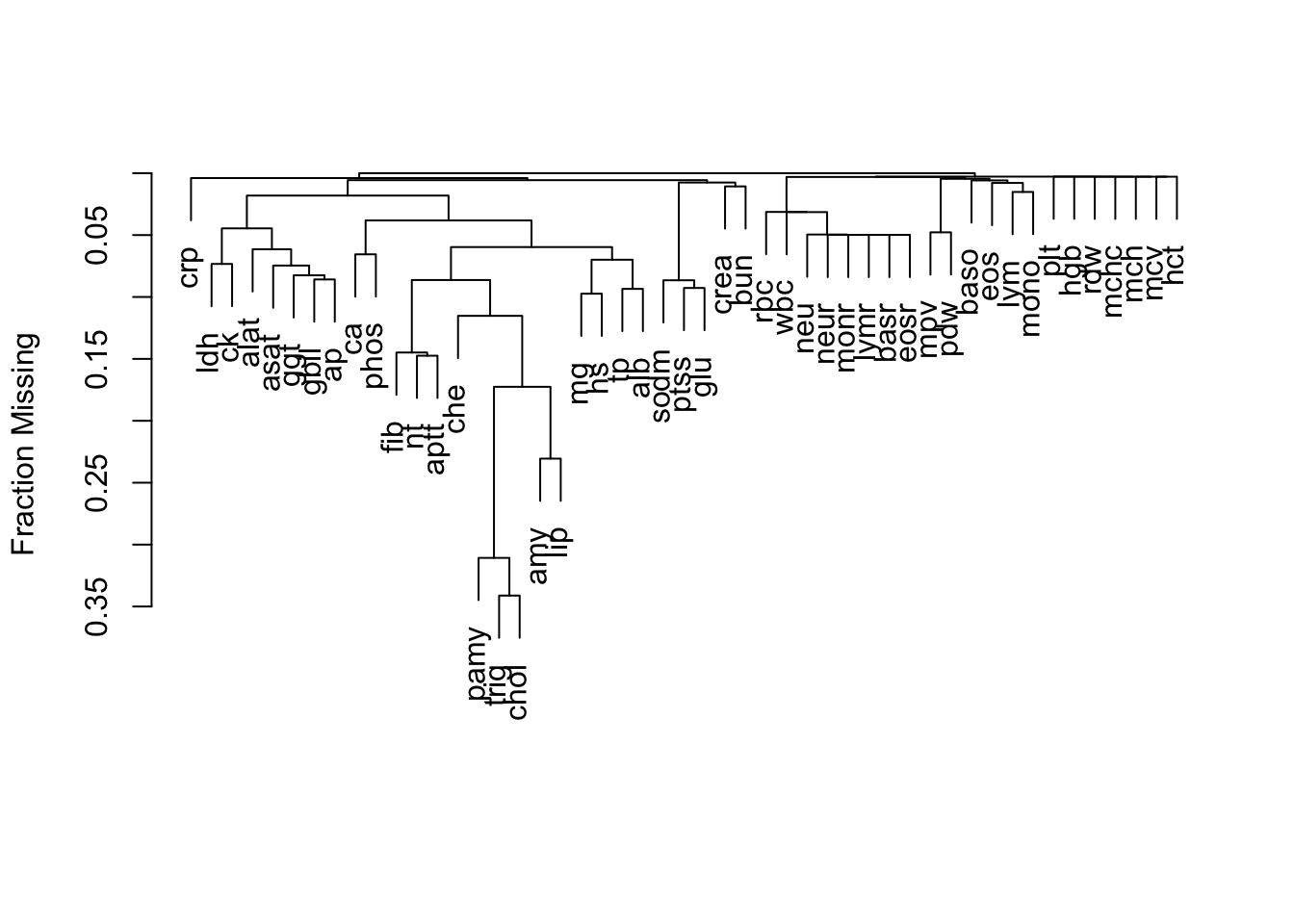
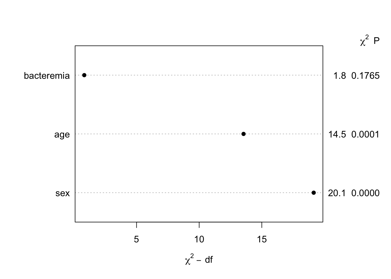
missChk(d, prednmiss=TRUE, omitpred='id')

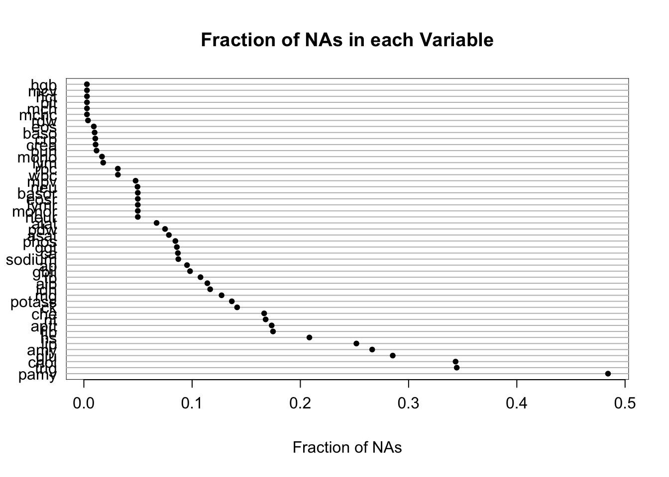
4 variables have no NAs and 49 variables have NAs

d has 14691 observations (3979 complete) and 53 variables (4 complete)

Number of NAs

	Minimum	Maximum	Mean
Per variable	0	7114	1354.5
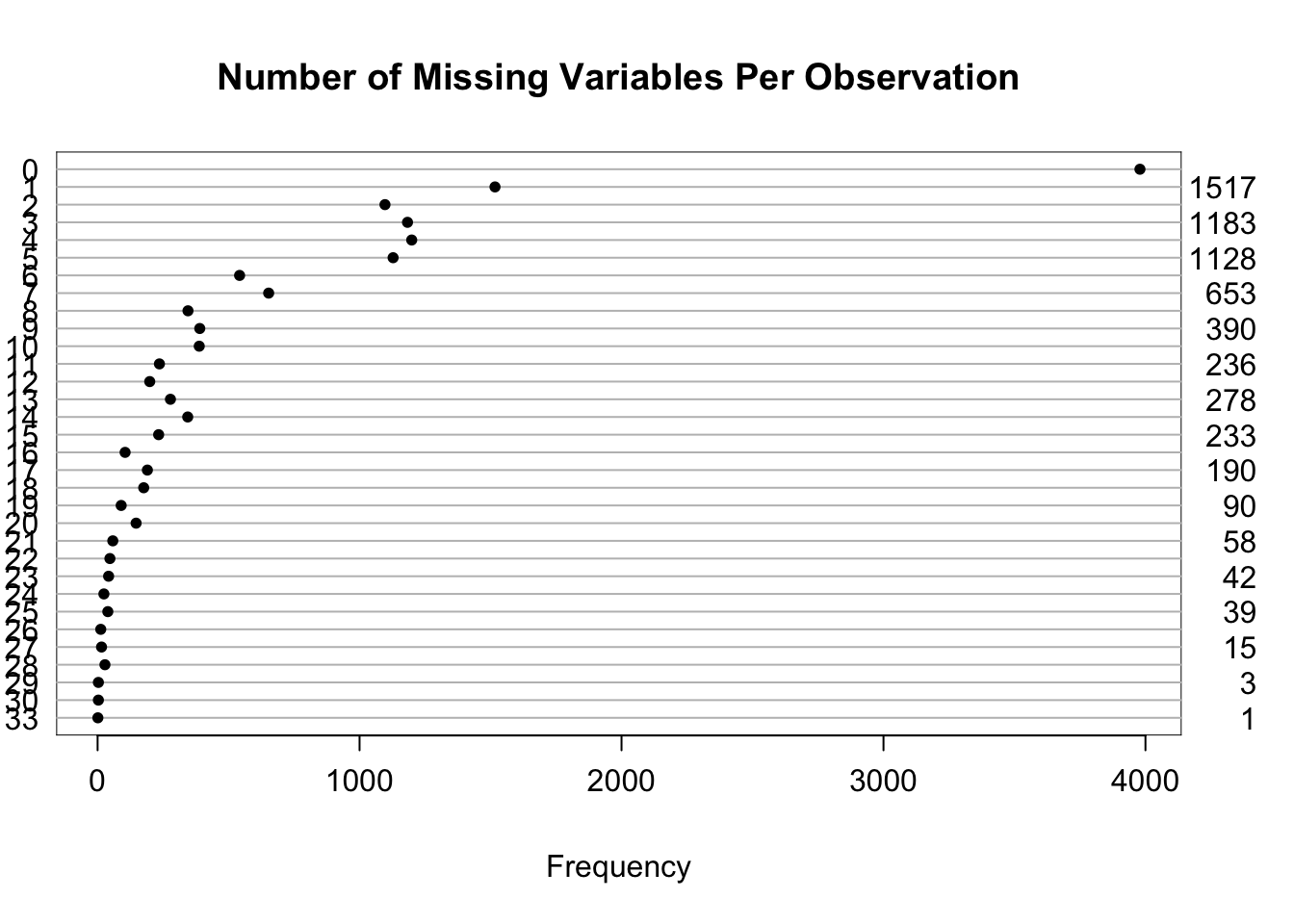
Per observation	0	33	4.9

Frequency distribution of number of NAs per variable

0	41	42	56	135	146	155	159	172	246	262	461	462	702	728	732	987	1102	1154	1242	1262	1276	1282	1400	1441	1583	1676	1714	1869	2008	2080	2447	2467	2549	2567	3061	3699	3913	4192	5045	5061	7114
4	1	5	1	1	1	1	1	1	1	1	1	1	1	1	5	1	1	1	1	1	1	1	1	1	1	1	1	1	1	1	1	1	1	1	1	1	1	1	1	1	1

Frequency distribution of number of incomplete variables per observation

0	1	2	3	4	5	6	7	8	9	10	11	12	13	14	15	16	17	18	19	20	21	22	23	24	25	26	27	28	29	30	33
3979	1517	1097	1183	1199	1128	542	653	345	390	388	236	199	278	344	233	105	190	176	90	147	58	47	42	24	39	12	15	28	3	3	1

NAs/var

Figure 24.1: Missing data patterns in d

NAs/obs

Mean # var NA when other var NA

NAs/var vs mean # other variables NA

Clustering of missingness

Sequential

Sequential frequency-ordered exclusions due to NAs

pamy	glu	pdw	ldh	trig	nt	hs	lip	basor	aptt	ck	phos	che	fib	amy	crp	tp	alat	gbil	potass	ggt	rdw	ca	chol	mg	crea	alb	asat
7114	1445	481	405	336	287	142	114	68	56	51	46	46	39	30	12	9	8	6	4	3	2	2	2	1	1	1	1

Predicting # NAs per obs

Logistic Regression Model

rms::lrm(formula = as.formula(form), data = d)

Frequencies of Responses

   0    1    2    3    4    5    6    7    8    9   10   11   12   13   14   15 
3979 1517 1097 1183 1199 1128  542  653  345  390  388  236  199  278  344  233 
  16   17   18   19   20   21   22   23   24   25   26   27   28   29   30   33 
 105  190  176   90  147   58   47   42   24   39   12   15   28    3    3    1 

	Model Likelihood Ratio Test	Discrimination Indexes	Rank Discrim. Indexes
Obs 14691	LR χ2 36.72	R2 0.003	C 0.519
max |∂log L/∂β| 3×10-9	d.f. 3	R23,14691 0.002	Dxy 0.037
	Pr(>χ2) <0.0001	R23,14351.2 0.002	γ 0.037
		Brier 0.062	τa 0.033

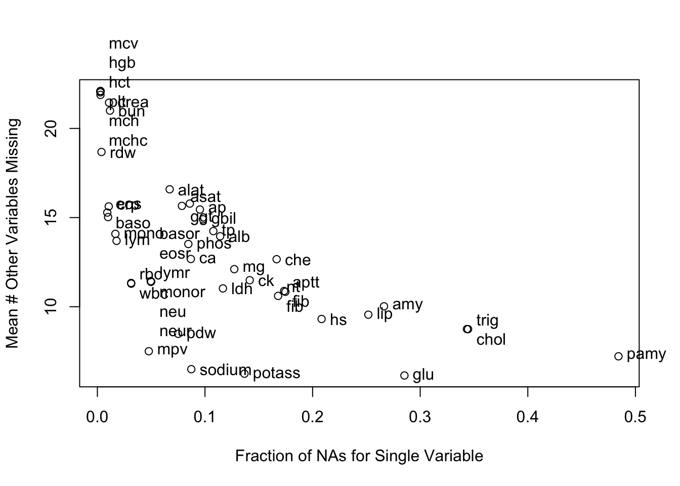
From the last tab, age and sex are predictors of the number of missing variables per observation, but the associations are very weak.

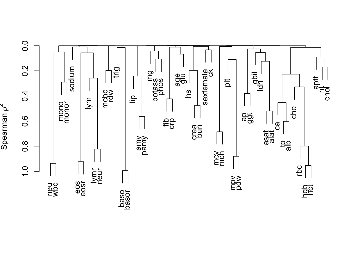
24.2 Variable Clustering

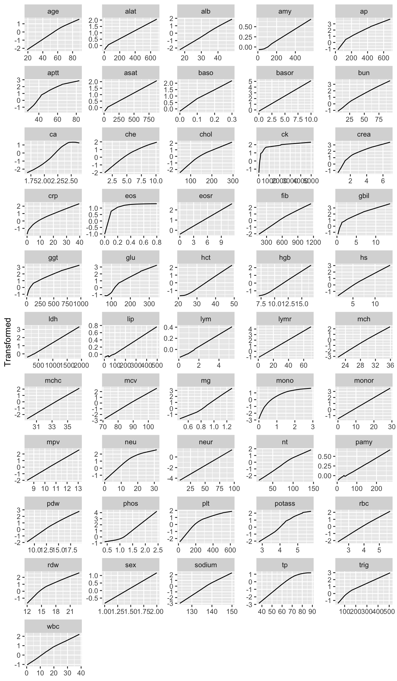
The R Hmisc package transace function, which uses the ACE (alternating conditional expectation) algorithm, is used to transform all the continuous variables. Transformations use nonparametric smoothers and are allowed to be non-monotonic. Transformation solutions maximize the \(R^2\) which with each variable can be predicted from the other variables, optimally transformed. The transformed variables are used in redundancy analysis and sparse principal components analysis. Bacteremia and subject id are not used in these unsupervised learning procedures.

To be more efficient, use multiple (5) imputations with predictive mean matching so that vClus will stack all the filled-in datasets before running the redundancy and PCA which are run on the single tall dataset, which contains no NAs. The correlation matrix and varclus results are already efficient because they use pairwise deletion of NAs.

Because transformed variables are passed to the redundancy analysis, variables are not expanded into splines in that analysis (see nk=0 below).

Here is the order in which vClus does things:

• clustering with pairwise NA deletion
• complete datasets using aregImpute output, stack them, use stacked data for all that follows
• transace
• redun
• sparce PCA

n <- setdiff(names(d), 'id')
n[n == 'baso'] <- 'I(baso)'
f <- as.formula(paste('~', paste(n, collapse='+')))
if(! file.exists('bacteremia-aregimpute.rds')) {
  set.seed(1)
  a <- aregImpute(f, data=d, n.impute=5)
  saveRDS(a, 'bacteremia-aregimpute.rds')
  } else a <- readRDS('bacteremia-aregimpute.rds')

1

all variables other than id

2

force baso to be linear in multiple imputation because of ties

3

aregImpute ran about 15 minutes when

4

so that multiple imputations reproduce

v <- vClus(d, fracmiss=0.8, corrmatrix=TRUE,
           trans=TRUE, redundancy=TRUE, spc=TRUE,
           exclude = ~ id + bacteremia,
           imputed=a,
           redunargs=list(nk=0),
           spcargs=list(k=20, sw=TRUE, nvmax=5), # sparse PCA 5m
           transacefile='bacteremia-transace.rds',
           spcfile='bacteremia-spc.rds')   # uses previous run if no inputs changed

Correlation Matrix

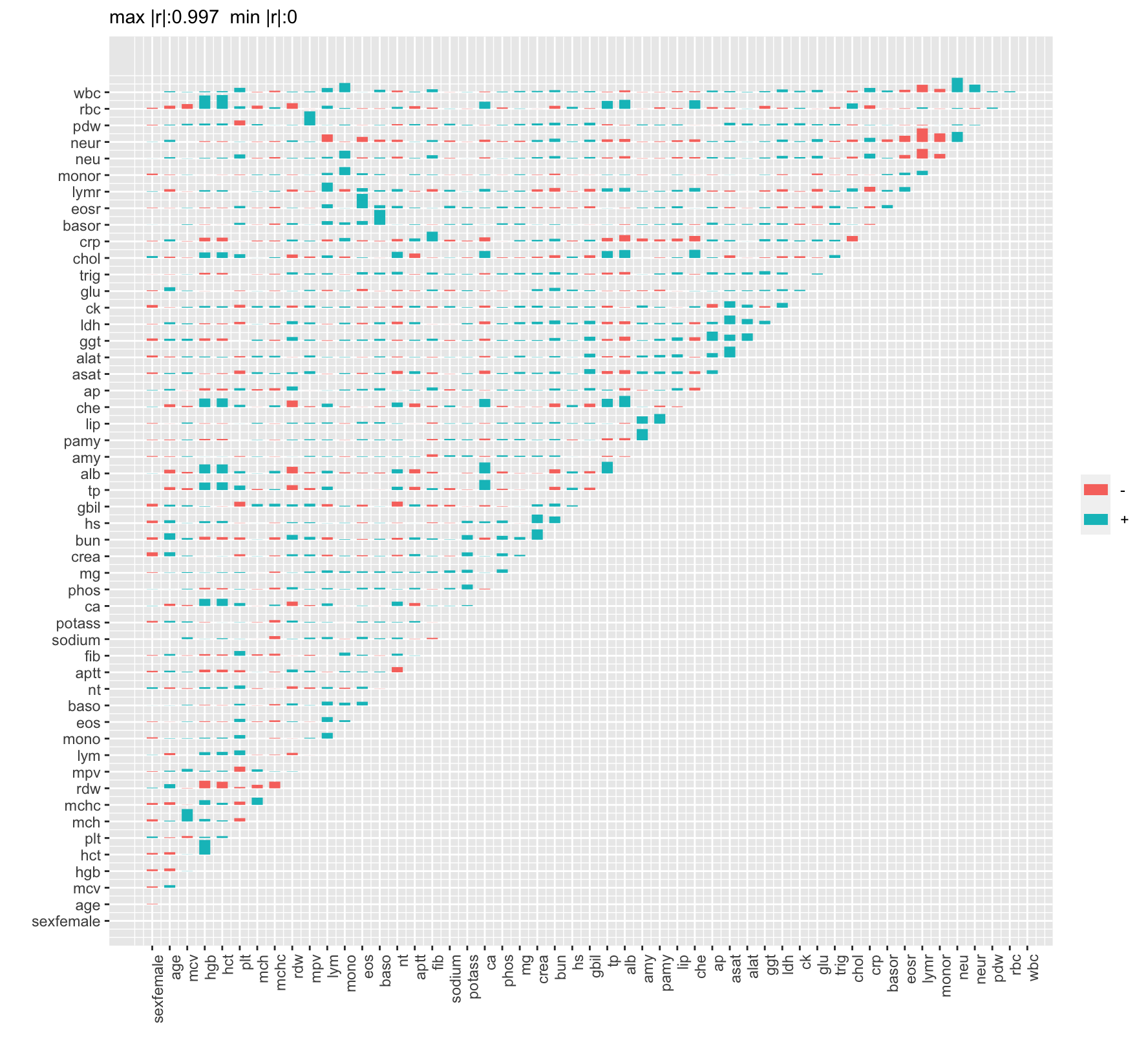
Figure 24.2: Spearman rank correlation matrix. Positive correlations are blue and negative are red.

Variable Clustering

Re-run because of changes in the following objects: args

 
 Redundancy Analysis
 
 n: 73455   p: 51   nk: 0 
 
 Number of NAs:  0 
 
 Transformation of target variables forced to be linear
 
 R-squared cutoff: 0.9  Type: ordinary 
 
 R^2 with which each variable can be predicted from all other variables:
 
    sex    age    mcv    hgb    hct    plt    mch   mchc    rdw    mpv    lym   mono 
  0.190  0.281  0.995  0.991  0.992  0.503  0.996  0.984  0.505  0.892  0.813  0.625 
    eos   baso     nt   aptt    fib sodium potass     ca   phos     mg   crea    bun 
  0.294  0.538  0.375  0.242  0.652  0.256  0.237  0.605  0.343  0.214  0.651  0.717 
     hs   gbil     tp    alb    amy   pamy    lip    che     ap   asat   alat    ggt 
  0.432  0.394  0.747  0.838  0.811  0.524  0.708  0.664  0.558  0.802  0.686  0.539 
    ldh     ck    glu   trig   chol    crp  basor   eosr   lymr  monor    neu   neur 
  0.648  0.269  0.146  0.275  0.545  0.658  0.976  0.994  0.999  0.997  0.829  1.000 
    pdw    rbc    wbc 
  0.893  0.962  0.873 
 
 Rendundant variables:
 
 neur mch hct hgb
 
 
 Predicted from variables:
 
 sex age mcv plt mchc rdw mpv lym mono eos baso nt aptt fib sodium potass ca
 phos mg crea bun hs gbil tp alb amy pamy lip che ap asat alat ggt ldh ck
 glu trig chol crp basor eosr lymr monor neu pdw rbc wbc
 
   Variable Deleted   R^2 R^2 after later deletions
 1             neur 1.000                     1 1 1
 2              mch 0.996               0.996 0.996
 3              hct 0.992                     0.958
 4              hgb 0.949                           

htmlVerbatim(v$transace)

 
 Transformations Using Alternating Conditional Expectation
 
 ~sex + age + mcv + hgb + hct + plt + mch + mchc + rdw + mpv + 
     lym + mono + eos + baso + nt + aptt + fib + sodium + potass + 
     ca + phos + mg + crea + bun + hs + gbil + tp + alb + amy + 
     pamy + lip + che + ap + asat + alat + ggt + ldh + ck + glu + 
     trig + chol + crp + basor + eosr + lymr + monor + neu + neur + 
     pdw + rbc + wbc
 
 
 n= 73455
 
 Transformations:
 
         sex         age         mcv         hgb         hct         plt         mch 
 categorical     general     general     general     general     general     general 
        mchc         rdw         mpv         lym        mono         eos        baso 
     general     general     general     general     general     general     general 
          nt        aptt         fib      sodium      potass          ca        phos 
     general     general     general     general     general     general     general 
          mg        crea         bun          hs        gbil          tp         alb 
     general     general     general     general     general     general     general 
         amy        pamy         lip         che          ap        asat        alat 
     general     general     general     general     general     general     general 
         ggt         ldh          ck         glu        trig        chol         crp 
     general     general     general     general     general     general     general 
       basor        eosr        lymr       monor         neu        neur         pdw 
     general     general     general     general     general     general     general 
         rbc         wbc 
     general     general 
 
 
 R-squared achieved in predicting each variable:
 
    sex    age    mcv    hgb    hct    plt    mch   mchc    rdw    mpv    lym   mono 
  0.275  0.405  0.995  0.992  0.992  0.547  0.996  0.983  0.552  0.897  0.844  0.870 
    eos   baso     nt   aptt    fib sodium potass     ca   phos     mg   crea    bun 
  0.904  0.605  0.384  0.275  0.663  0.288  0.274  0.619  0.412  0.237  0.675  0.730 
     hs   gbil     tp    alb    amy   pamy    lip    che     ap   asat   alat    ggt 
  0.486  0.429  0.773  0.850  0.814  0.532  0.714  0.677  0.583  0.811  0.693  0.609 
    ldh     ck    glu   trig   chol    crp  basor   eosr   lymr  monor    neu   neur 
  0.660  0.431  0.183  0.348  0.564  0.678  0.976  0.994  0.999  0.997  0.919  1.000 
    pdw    rbc    wbc 
  0.899  0.978  0.899  

saveRDS(v, '/tmp/v.rds')

ggplot(v$transace, nrow=12)

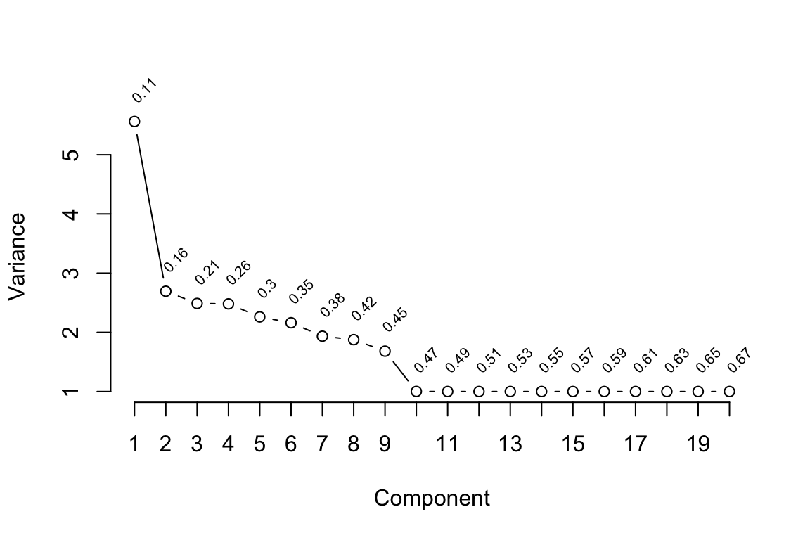
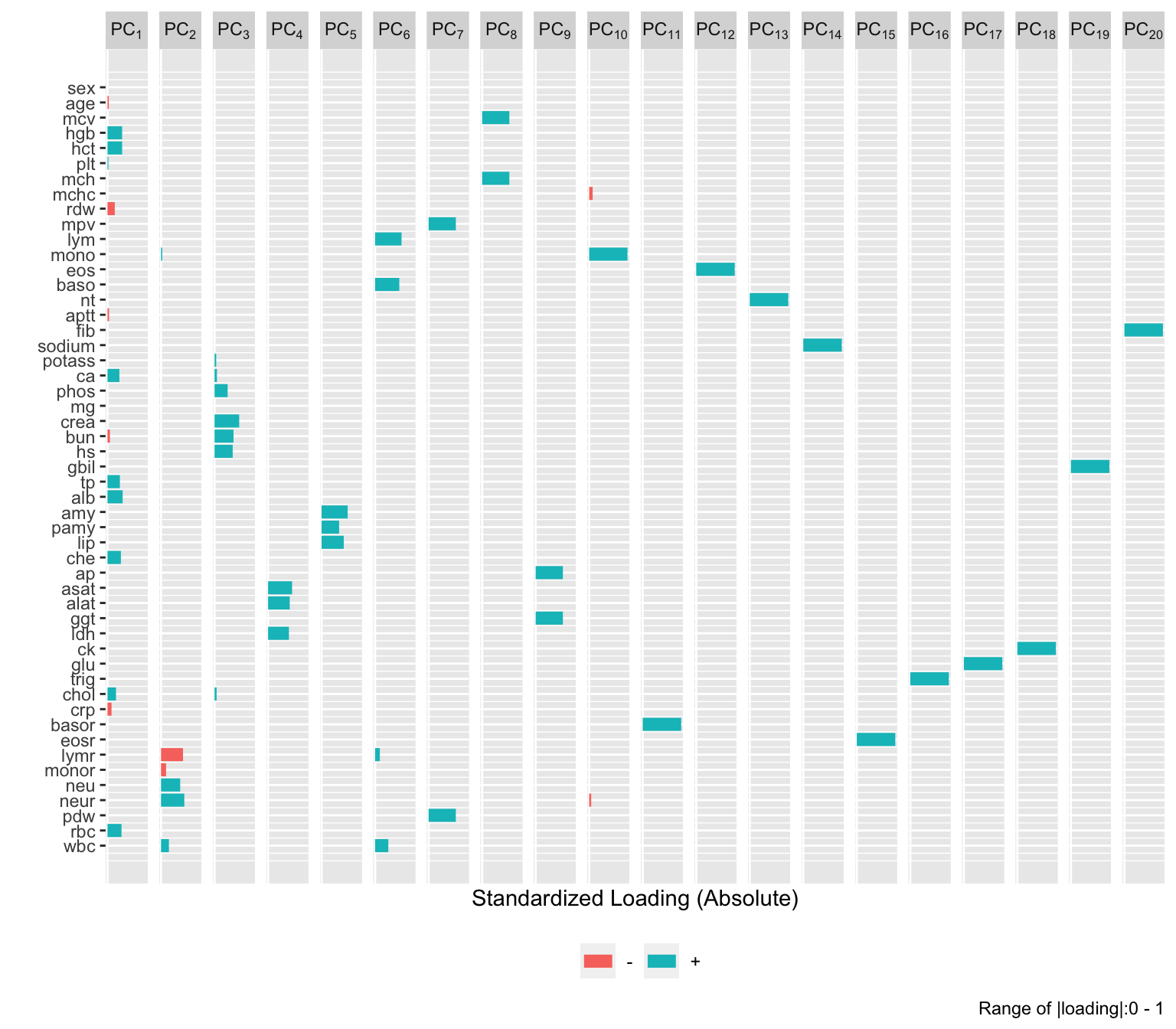
p <- v$princmp
# Print and plot sparse PC results
print(p)

Sparse Principal Components Analysis

Stepwise Approximations to PCs With Cumulative R^2

PC 1 
alb (0.767) + hct (0.943) + chol (0.96) + che (0.969) + ca (0.979)

PC 2 
neur (0.849) + neu (0.974) + lymr (0.989) + wbc (0.998) + monor (1)

PC 3 
crea (0.811) + hs (0.908) + phos (0.961) + bun (0.996) + ca (0.999)

PC 4 
asat (0.917) + ldh (0.959) + alat (1)

PC 5 
amy (0.935) + pamy (0.957) + lip (1)

plot(p)

plot(v$p, 'loadings', nrow=1)

Morris, T. P., White, I. R., Carpenter, J. R., Stanworth, S. J., & Royston, P. (2015). Combining fractional polynomial model building with multiple imputation: T. P. Morris et Al . Statist. Med., 34(25), 3298–3317. https://doi.org/10.1002/sim.6553