Original source: Generalized body composition prediction equation for men using simple measurement techniques, K.W. Penrose, A.G. Nelson, A.G. Fisher, FACSM, Human Performance Research Center, Brigham Young University, Provo, Utah 84602 as listed in Medicine and Science in Sports and Exercise, vol. 17, no. 2, April 1985, p. 189
Response variable is proportion of body mass that composed of fat
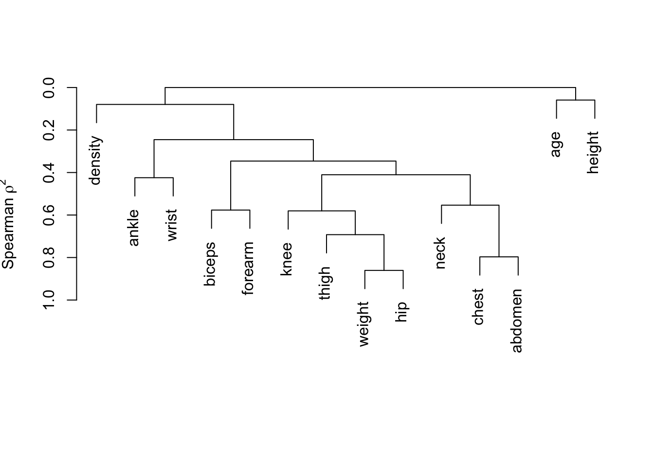
Display descriptive statistics and variable clustering pattern
Run a redundancy analysis
Knowing that abdomen circumference is a dominating predictor and that height must be taken into account when interpreting it, learn about the transformations of the variables from a linear model with predictors abdomen, height, and age
Compare 4 competing models with AIC
Assess the contribution of all other size measurements in predicting fat
15 Continous Variables of 15 Variables, 249 Observations
Variable
Label
Units
n
Missing
Distinct
Info
Mean
Gini |Δ|
Quantiles
.05 .10 .25 .50 .75 .90 .95
density
Density
g/cm3
249
0
216
1.000
1.055
0.02119
1.026 1.032 1.041 1.055 1.070 1.080 1.085
fat
Body Fat
Proportion
249
0
174
1.000
0.1925
0.09364
0.0630 0.0850 0.1250 0.1920 0.2530 0.2992 0.3248
age
Age
years
249
0
51
0.999
44.95
14.39
25.0 27.0 36.0 43.0 54.0 63.2 67.0
weight
Weight
kg
249
0
194
1.000
81.39
14.27
62.67 67.17 72.30 80.24 89.44 98.52 102.58
height
Height
cm
249
0
47
0.999
178.7
7.541
167.9 170.7 174.0 178.4 183.5 187.3 189.2
neck
Neck Circumference
cm
249
0
89
1.000
38.03
2.66
34.34 35.20 36.40 38.00 39.50 40.92 41.86
chest
Chest Circumference
cm
249
0
171
1.000
100.9
9.241
89.20 91.36 94.60 99.70 105.30 112.32 116.52
abdomen
Abdomen Circumference at Umbilicus
cm
249
0
183
1.000
92.67
11.73
77.60 79.68 85.20 91.00 99.20 105.76 110.88
hip
Hip Circumference
cm
249
0
150
1.000
99.94
7.422
89.36 92.06 95.60 99.30 103.50 108.64 111.86
thigh
Thigh Circumference
cm
249
0
137
1.000
59.45
5.619
51.52 53.24 56.10 59.00 62.30 65.84 68.46
knee
Knee Circumference
cm
249
0
89
1.000
38.61
2.638
34.90 35.68 37.10 38.50 39.90 41.70 42.66
ankle
Ankle Circumference
cm
249
0
60
0.999
23.12
1.694
21.00 21.50 22.00 22.80 24.00 24.82 25.46
biceps
Extended Biceps Circumference
cm
249
0
103
1.000
32.32
3.363
27.74 28.80 30.30 32.10 34.40 36.24 37.20
forearm
Forearm Circumference
cm
249
0
76
1.000
28.69
2.235
25.74 26.28 27.30 28.80 30.00 31.10 31.76
wrist
Wrist Circumference
cm
249
0
44
0.998
18.25
1.039
16.84 17.08 17.60 18.30 18.80 19.40 19.80
Code
plot(varclus(~ . - fat, data=d))
Do a redundancy analysis
Code
r <-redun(fat ~ ., data=d)r
Redundancy Analysis

fat ~ .

n: 249  p: 15   nk: 3

Number of NAs:   0

Transformation of target variables forced to be linear

R-squared cutoff: 0.9   Type: ordinary

R^2 with which each variable can be predicted from all other variables:

    fat density     age  weight  height    neck   chest abdomen     hip   thigh
  0.983   0.981   0.605   0.983   0.749   0.788   0.919   0.950   0.938   0.892
   knee   ankle  biceps forearm   wrist
  0.800   0.502   0.744   0.592   0.769

Rendundant variables:

fat weight abdomen


Predicted from variables:

density age height neck chest hip thigh knee ankle biceps forearm wrist

  Variable Deleted   R^2 R^2 after later deletions
1              fat 0.983               0.983 0.982
2           weight 0.983                     0.981
3          abdomen 0.944
Code
# Show strongest relationships among transformed predictorsr2describe(r$scores, nvmax=4)
Strongest Predictors of Each Variable With Cumulative R^2

fat
density (0.975) + chest (0.977) + age (0.978) + biceps (0.978)

density
fat (0.975) + wrist (0.976) + ankle (0.976) + height (0.976)

age
fat (0.084) + thigh (0.276) + wrist (0.416) + abdomen (0.461)

weight
hip (0.888) + chest (0.927) + height (0.96) + neck (0.968)

height
knee (0.247) + density (0.363) + weight (0.429) + abdomen (0.529)

neck
weight (0.69) + wrist (0.728) + height (0.741) + hip (0.755)

chest
abdomen (0.836) + weight (0.868) + hip (0.879) + height (0.893)

abdomen
chest (0.836) + density (0.893) + hip (0.927) + age (0.937)

hip
weight (0.888) + thigh (0.91) + abdomen (0.918) + neck (0.923)

thigh
hip (0.795) + age (0.821) + biceps (0.843) + knee (0.853)

knee
weight (0.721) + ankle (0.734) + thigh (0.745) + height (0.758)

ankle
weight (0.37) + abdomen (0.41) + wrist (0.435) + knee (0.453)

biceps
weight (0.633) + forearm (0.684) + thigh (0.7) + neck (0.707)

forearm
biceps (0.452) + wrist (0.491) + age (0.508) + neck (0.518)

wrist
neck (0.546) + ankle (0.604) + age (0.636) + height (0.66)
weight could be dispensed with but we will keep it for historical reasons.
23.2 Learn Predictor Transformations and Interactions From Simple Model
Compare AICs of 5 competing models
It is safe to use AIC to select from among perhaps 3 models so we are pushing the envelope here
How does this translate to improvement in median prediction error?
Code
median(abs(resid(f)))
[1] 0.03283904
Code
median(abs(resid(g)))
[1] 0.02995479
There is a reduction of 0.003 in the typical prediction error
Proportion of fat varies from 0.06 - 0.32 (0.05 quantile to 0.95 quantile)
Additional variables are not worth it
A typical prediction error of 0.03 makes the model fit for purpose
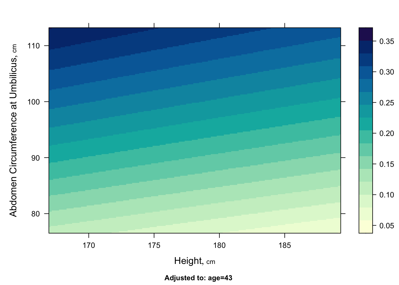
23.4 Model Interpretation
Image plot
Nomogram
Code
p <-Predict(f, height, abdomen)bplot(p, ylabrot=90)
Code
plot(nomogram(f), lplab='Fat Fraction')
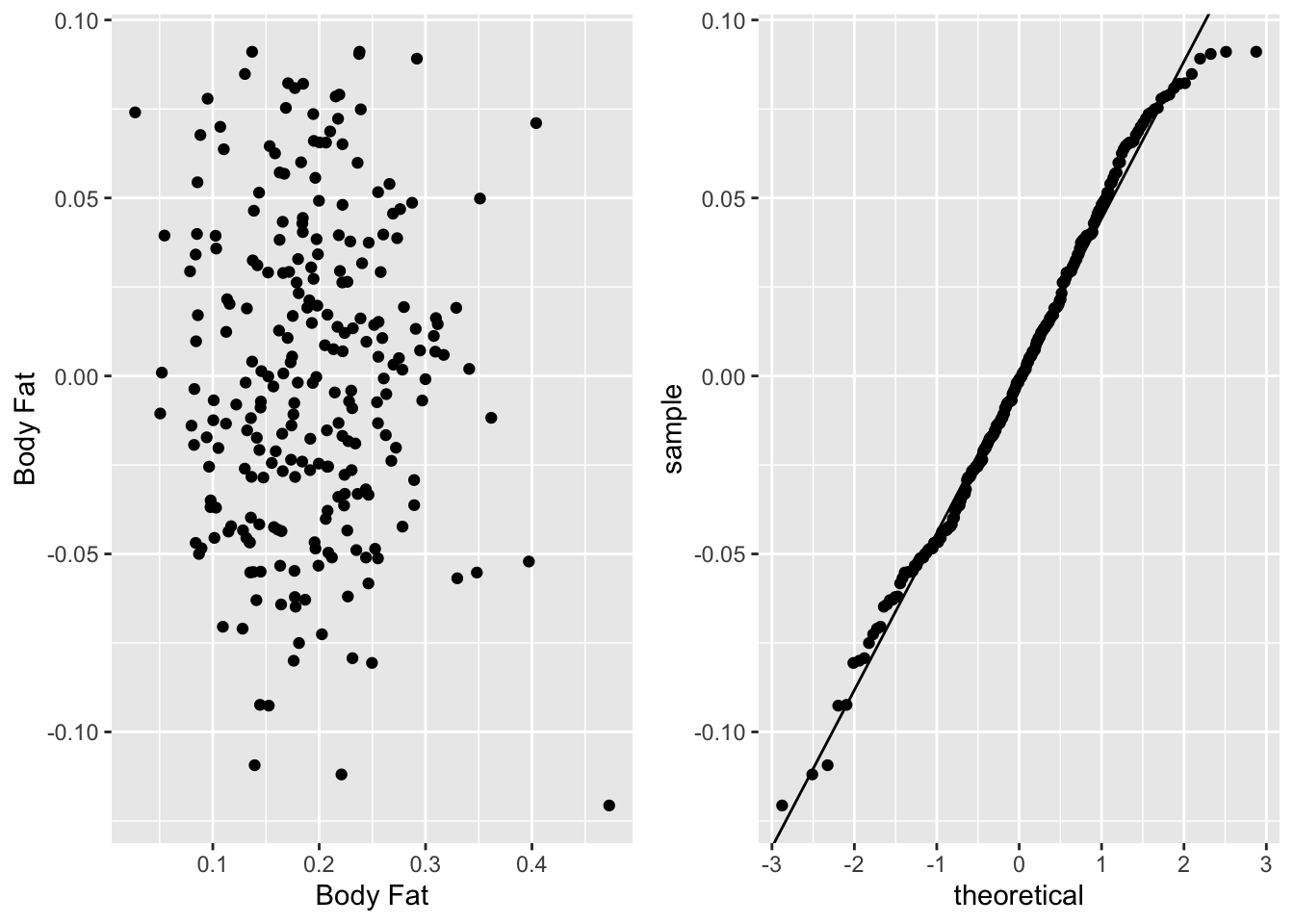
Source Code
```{r include=FALSE}require(rms)require(ggplot2)options(qproject='rms', prType='html')require(qreport)getRs('qbookfun.r')hookaddcap()knitr::set_alias(w = 'fig.width', h = 'fig.height', cap = 'fig.cap', scap ='fig.scap')```# Body Fat: Case Study in Linear Modeling {#sec-bodyfat}* Goal: accurately estimate proportion of male adult body mass that is fat using readily available body dimensions and age* Gold standard body fat was determined by underwater weighing* Source: [`kaggle` competition](https://www.kaggle.com/datasets/fedesoriano/body-fat-prediction-dataset)* Original source: Generalized body composition prediction equation for men using simple measurement techniques, K.W. Penrose, A.G. Nelson, A.G. Fisher, FACSM, Human Performance Research Center, Brigham Young University, Provo, Utah 84602 as listed in Medicine and Science in Sports and Exercise, vol. 17, no. 2, April 1985, p. 189* 252 men; 3 excluded due to erroneous data* Available at [hbiostat.org/data](https://hbiostat.org/data) or using `getHdata`**Statistical Analysis Attack*** Response variable is proportion of body mass that composed of fat* Display descriptive statistics and variable clustering pattern* Run a redundancy analysis* Knowing that abdomen circumference is a dominating predictor and that height must be taken into account when interpreting it, learn about the transformations of the variables from a linear model with predictors abdomen, height, and age* Compare 4 competing models with AIC* Assess the contribution of all other size measurements in predicting fat## Descriptive Statistics```{r}getHdata(bodyfat)d <- bodyfatdd <-datadist(d); options(datadist='dd')des <-describe(d)sparkline::sparkline(0) # load jQuery javascript for sparklinesprint(des, which='continuous')plot(varclus(~ . - fat, data=d))```Do a redundancy analysis```{r}r <-redun(fat ~ ., data=d)r# Show strongest relationships among transformed predictorsr2describe(r$scores, nvmax=4)````weight` could be dispensed with but we will keep it for historical reasons.## Learn Predictor Transformations and Interactions From Simple Model* Compare AICs of 5 competing models* It is safe to use AIC to select from among perhaps 3 models so we are pushing the envelope here```{r}AIC(ols(fat ~rcs(age, 4) +rcs(height, 4) *rcs(abdomen, 4), data=d))AIC(ols(fat ~rcs(age, 4) +rcs(log(height), 4) +rcs(log(abdomen), 4), data=d))AIC(ols(fat ~rcs(age, 4) +log(height) +log(abdomen), data=d))AIC(ols(fat ~ age * (log(height) +log(abdomen)), data=d))AIC(ols(fat ~ age + height + abdomen, data=d))```* Third model has lowest AIC* Will use its structure when adding other predictors* Check contant variance and normality assumptions on the winning small model```{r}f <-ols(fat ~rcs(age, 4) +log(height) +log(abdomen), data=d)fpdx <-function() { r <-resid(f) w <-data.frame(r=r, fitted=fitted(f)) p1 <-ggplot(w, aes(x=fitted, y=r)) +geom_point() p2 <-ggplot(w, aes(sample=r)) +stat_qq() +geom_abline(intercept=mean(r), slope=sd(r)) gridExtra::grid.arrange(p1, p2, ncol=2)}pdx()```* Normal and constant variance (across predicted values) on the original fat scale* Usually would need to transform a [0,1]-restricted variable* Luckily no predicted values outside [0,1] in the dataset* Will keep a linear model on untransformed fat## Assess Predictive Discrimination Added by Other Size Variables```{r}g <-ols(fat ~rcs(age, 4) +log(height) +log(abdomen) +log(weight) +log(neck) +log(chest) +log(hip) +log(thigh) +log(knee) +log(ankle) +log(biceps) +log(forearm) +log(wrist), data=d)AIC(g)```* By AIC the large model is better* $R^{2}_\text{adj}$ went from 0.704 to 0.733* How does this translate to improvement in median prediction error?```{r}median(abs(resid(f)))median(abs(resid(g)))```* There is a reduction of 0.003 in the typical prediction error* Proportion of fat varies from 0.06 - 0.32 (0.05 quantile to 0.95 quantile)* Additional variables are not worth it* A typical prediction error of 0.03 makes the model fit for purpose## Model Interpretation* Image plot* Nomogram```{r}p <-Predict(f, height, abdomen)bplot(p, ylabrot=90)plot(nomogram(f), lplab='Fat Fraction')``````{r echo=FALSE}saveCap('23')```