```{r include=FALSE}
require(Hmisc)
options(qproject='rms', prType='html')
require(qreport)
getRs('qbookfun.r')
hookaddcap()
knitr::set_alias(w = 'fig.width', h = 'fig.height', cap = 'fig.cap', scap ='fig.scap')
options(omitlatexcom=TRUE) # makes latex() not generate comments
```
# Cox Proportional Hazards Regression Model {#sec-cox}
## Model
### Preliminaries
* Most popular survival model
* Semi-parametric (nonparametric hazard; parametric regression)
* Usually more interest in effects of $X$ than on shape of $\lambda(t)$
* Uses only rank ordering of failures/censoring times $\rightarrow$
more robust, easier to write protocol
* Even if parametric PH assumptions true, Cox still fully
efficient for $\beta$
* Model diagnostics are advanced
* Log-rank test is a special case with one binary $X$
* The Cox model is a special case of ordinal semiparametric models (@sec-ordsurv) although it has better model diagnostics, especially for assessing proportional hazards
### Model Definition
$$
\lambda(t|X) = \lambda(t) \exp(X\beta) .
$$
* No intercept parameter
* Shape of $\lambda$ not important
* When a predictor say $X_1$ is
+ binary
+ doesn't interact with other predictors
+ has coefficient $\beta_1$
+ satisfies the proportional hazards (PH) assumption so that $X_1$ does not interact with time $\rightarrow$ hazard ratio (HR) $\exp(\beta_{1})$ is the ratio of hazard functions for $X_{1}=1$ vs. $X_{1}=0$
+ $\lambda(t)$ cancels out
+ by the PH assumption, the HR does not depend on $t$; $X_1$ has a constant effect on $\lambda$ over time
+ under PH and absence of covariate interactions, HR is a good overall effect estimate for binary $X_1$
HR is the ratio of two instantaneous event rates
### Estimation of $\beta$ {#sec-cox-partial-like}
* The objective function to optimize is the Cox's partial likelihood function
* Partial likelihood only covers the $\beta$ part of the model, not the $\lambda$ or underlying survival curve part
+ these are estimated in a separate step once $\hat{\beta}$ is obtained
* Obtain maximum likelihood estimates of $\beta$ (formally, maximum partial likelihood estimates)
* See text for details
### Model Assumptions and Interpretation of Parameters
* Similar to other models; interpretation is on the log relative hazard scale
* Equivalent to using $\log(-\log(S(t)))$ scale
* HR of 2 is equivalent to raising the entire survival curve for a control subject to the second power to get the survival curve for an exposed subject
+ Example: if a control subject has 5y survival probability of 0.7 and the exposed:control HR is 2, the exposed subject has a 5y survival probability of 0.49
+ If the HR is $\frac{1}{2}$, the exposed subject has a survival curve that is the square root of the control, so S(5) would be $\sqrt{0.7} = 0.837$
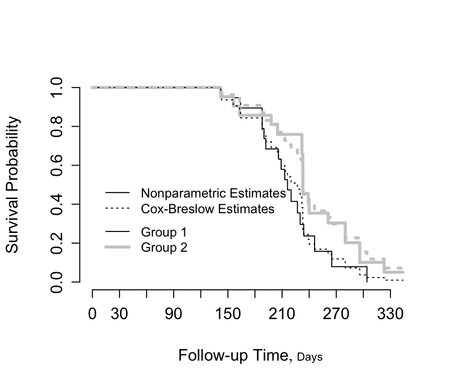
### Example
```{r kprats-cph-np,w=4.75,h=4,cap='Altschuler--Nelson--Fleming--Harrington nonparametric survival estimates and Cox-Breslow estimates for rat data [@pik66met]',scap='Nonparametric and Cox--Breslow survival estimates'}
#| label: fig-cox-kprats-cph-np
require(rms)
options(prType='html')
group <- c(rep('Group 1',19),rep('Group 2',21))
group <- factor(group)
dd    <-  datadist(group); options(datadist='dd')
days <-
  c(143,164,188,188,190,192,206,209,213,216,220,227,230,
    234,246,265,304,216,244,142,156,163,198,205,232,232,
    233,233,233,233,239,240,261,280,280,296,296,323,204,344)
death <- rep(1,40)
death[c(18,19,39,40)] <- 0
units(days) <- 'Day'
df <- data.frame(days, death, group)
S <- Surv(days, death)
f <- npsurv(S ~ group, type='fleming')
for(meth in c('exact', 'breslow', 'efron')) {
  g <- cph(S ~ group, method=meth, surv=TRUE, x=TRUE, y=TRUE)
  # print(g) to see results
}
f.exp <- psm(S ~ group, dist='exponential')
fw    <- psm(S ~ group, dist='weibull')
phform <- pphsm(fw)
co <- gray(c(0, .8))
survplot(f, lty=c(1, 1), lwd=c(1, 3), col=co,
         label.curves=FALSE, conf='none')
survplot(g, lty=c(3, 3), lwd=c(1, 3), col=co,  # Efron approx.
         add=TRUE, label.curves=FALSE, conf.type='none')
legend(c(2, 160), c(.38, .54),
       c('Nonparametric Estimates', 'Cox-Breslow Estimates'),
       lty=c(1, 3), cex=.8, bty='n')
legend(c(2, 160), c(.18, .34), cex=.8,
       c('Group 1', 'Group 2'), lwd=c(1,3), col=co, bty='n')
```
| Model | Group Regression Coefficient | S.E. | Wald p Value | Group 2:1 Hazard Ratio |
|-----|-----|-----|-----|-----|
| Cox (Exact) | -0.629 | 0.361 | 0.08 | 0.533 |
| Cox (Efron) | -0.569 | 0.347 | 0.10 | 0.566 |
| Cox (Breslow) | -0.596 | 0.348 | 0.09 | 0.551 |
| Exponential | -0.093 | 0.334 | 0.78 | 0.911 |
| Weibull (AFT) | 0.132 | 0.061 | 0.03 | |
| Weibull (PH) | -0.721 | | | 0.486 |
### Design Formulations
* $k-1$ dummies for $k$ treatments, one treatment $\rightarrow$ $\lambda(t)$
* Only provides relative effects
### Extending the Model by Stratification
* Is a unique feature of the Cox model
* Adjust for non-modeled factors
* Factors too difficult to model or fail PH assumption
* Commonly used in RCTs to adjust for site variation
* Allow form of $\lambda$ to vary across strata
* Rank failure times _within_ strata
* $b$ strata, stratum ID is $C$
\begin{array}{ccc}
\lambda(t|X, C=j) &=& \lambda_{j}(t) \exp(X\beta), {\rm\ \ \ or} \nonumber \\
S(t|X, C=j) &=& S_{j}(t)^{\exp(X\beta)}
\end{array}
* Not assume connection between shapes of $\lambda_j$
* By default, assume common $\beta$
* Ex: model age, stratify on sex <br>
Estimates common age slope pooling F and M <br>
No assumption about effect of sex except no age interact.
* Can stratify on multiple factors (cross-classify)
* Loss of efficiency not bad unless number of events in
strata very small
* Stratum with no events is ignored
* Estimate $\beta$ by getting separate log-likelihood for
each stratum and adding up (independence)
* No inference about strat. factors
* Useful for checking PH and linearity assumptions:
Model, then stratify on an $X$
* Can extend to strata $\times$ covariable interaction
\begin{array}{ccc}
\lambda(t|X_{1}, C=1) &=& \lambda_{1}(t)\exp(\beta_{1}X_{1}) \nonumber \\
\lambda(t|X_{1}, C=2) &=& \lambda_{2}(t)\exp(\beta_{1}X_{1}+\beta_{2}X_{1})
\end{array}
$$\lambda(t|X_{1}, C=j) = \lambda_{j}(t)\exp(\beta_{1}X_{1}+\beta_{2}X_{2})$$
* $X_2$ is product interaction term (0 for F, $X_1$ for M)
* Testing interaction with sex without modeling main effect!
## Estimation of Survival Probability and Secondary Parameters {#sec-cox-estimation}
* Kalbfleisch-Prentice discrete hazard model method $\rightarrow$
K-M if $\hat{\beta}=0$
* Breslow method $\rightarrow$ Nelson _et al._ if $\hat{\beta}=0$
$$\hat{S}(t|X) = \hat{S}(t)^{\exp(X\hat{\beta})}$$
* Stratified model $\rightarrow$ estimate underlying hazard parameters
separately within strata
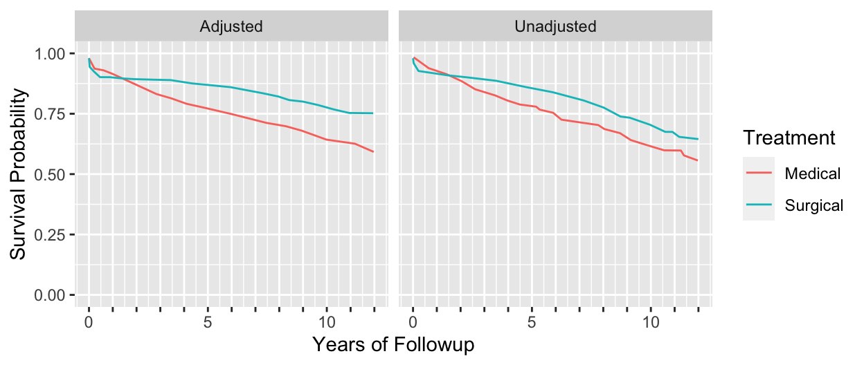
* "Adjusted K-M estimates"
```{r echo=FALSE, w=6.5, h=2.75}
#| label: fig-cox-cabg-adj
#| fig-scap: "Unadjusted (Kaplan--Meier) and adjusted survival estimates"
#| fig-cap: "Unadjusted (Kaplan--Meier) and adjusted (Cox--Kalbfleisch--Prentice) estimates of survival. Left, Kaplan--Meier estimates for patients treated medically and surgically at Duke University Medical Center from November $1969$ through December $1984$. These survival curves are not adjusted for baseline prognostic factors. Right, survival curves for patients treated medically or surgically after adjusting for all known important baseline prognostic characteristics [@cal89evo]."
require(ggplot2)
d <- readRDS('cox-cabg-adj.rds')
ggplot(d, aes(x=t, y=surv, color=Treatment)) + geom_line() +
facet_grid(~ Type) + ylim(0,1) + ylab('Survival Probability') +
xlab('Years of Followup') +
scale_x_continuous(breaks=0:12,
labels=c('0',rep('',4),'5',rep('',4),'10',
rep('',2)))
```
$$\hat{\Lambda}(t) = \sum_{i:t_{i}<t}\frac{d_{i}}{\sum_{Y_{i}\geq t_{i}}
\exp(X_{i}\hat{\beta})}$$
For any $X$, the estimates of $\Lambda$ and $S$ are
\begin{array}{ccc}
\hat{\Lambda}(t|X) &=& \hat{\Lambda}(t) \exp(X\hat{\beta}) \nonumber \\
\hat{S}(t|X) &=& \exp[-\hat{\Lambda}(t) \exp(X\hat{\beta}) ]
\end{array}
## Sample Size Considerations {#sec-cox-samsize}
* Consider case with no covariates and want to estimate $S(t)$; results to Kaplan-Meier
* As detailed in the text, one may need 184 subjects with an event, or censored late, to estimate $S(t)$ to within a margin of error of 0.1 everywhere, at the 0.95 confidence level
* Instead consider the case where the model has a single binary covariate and we want to estimate the hazard ratio to within a specified multiplicative margin of error (MMOE) with confidence $1 - \alpha$
* Assume equal sample size for $X=0$ and $X=1$ and let $e_0$ and $e_1$ denote the number of events in the two $X$ groups
* Variance of log HR is approximately $v=\frac{1}{e_{0}} + \frac{1}{e_{1}}$.
* Let $z$ denote the $1 - \alpha/2$ standard normal critical value
* MMOE with confidence $1 - \alpha$ is $\exp(z \sqrt{v})$
* To achieve a MMOE of 1.2 in estimating $e^{\hat{\beta}}$ with equal numbers of
events in the two groups and $\alpha=0.05$ requires a total of 462 events:
```{r mmoebeta}
z <- qnorm(1 - .05/2)
# v = (log(mmoe) / z) ^ 2
# If e0=e1=e/2, e=4/k
mmoe <- 1.2
k <- (log(mmoe) / z) ^ 2
4/k
```
* Sample size for external validation: at least 200 events [@col16sam]
## Test Statistics
* Score test = log-rank $\chi^2$ test statistic
* Score test in a stratified PH model is the stratified log-rank statistic
## Residuals
| Residual | Purposes |
|-----|-----|
| martingale | Assessing adequacy of a hypothesized predictor transformation; Graphing an estimate of a predictor transformation (@sec-cox-regression-assumptions) |
| score | Detecting overly influential observations |
| Schoenfeld | Testing PH assumption (@sec-cox-ph); graphing estimate of hazard ratio function (@sec-cox-ph) |
## Assessment of Model Fit
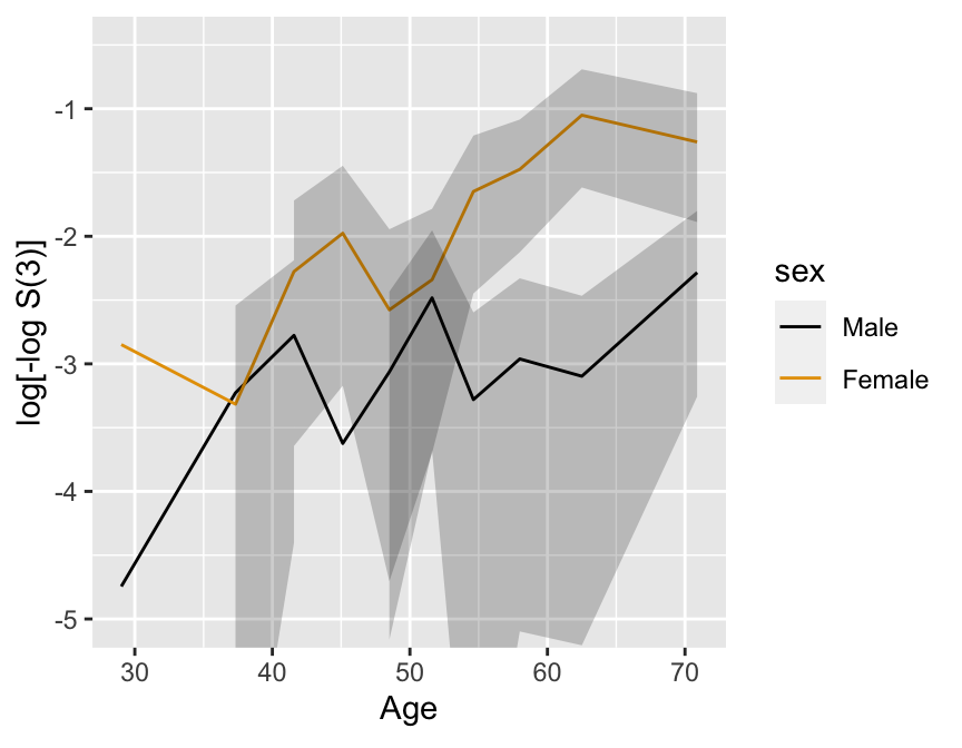
### Regression Assumptions {#sec-cox-regression-assumptions}
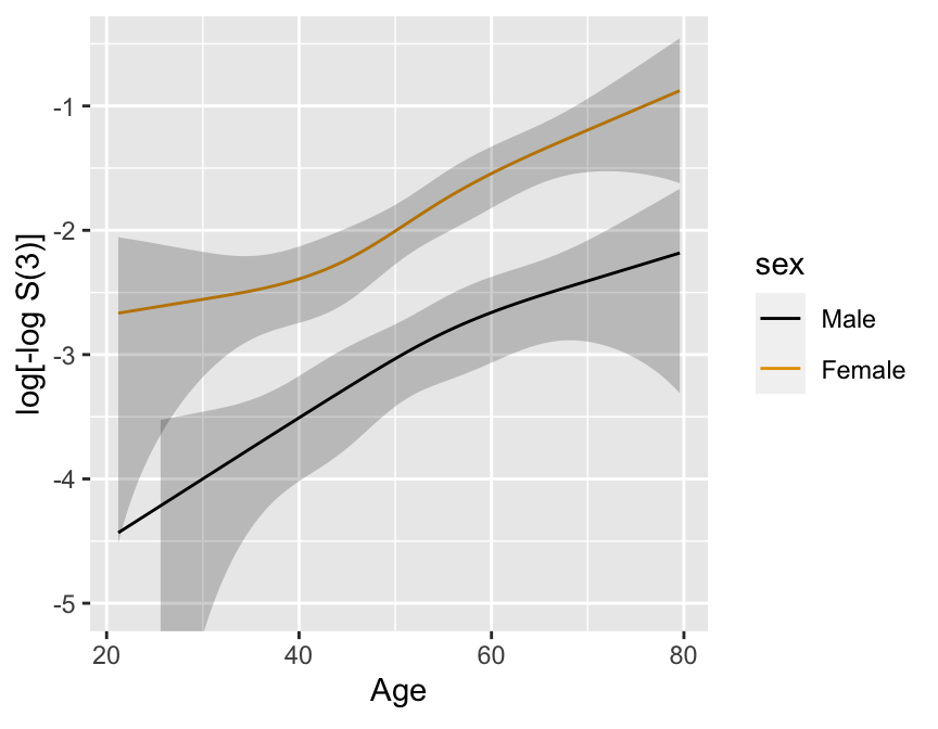
* Stratified KM estimates have problems
* 2000 simulated subject, $d=368$, 1196 M, 804 F
* Exponential with known log hazard, linear in age, additive in
sex
$$\lambda(t|X_{1},X_{2}) = .02 \exp[.8X_{1}+.04(X_{2}-50)]$$
```{r km-age-sex,w=4.5,h=3.5,cap='Kaplan--Meier log $\\Lambda$ estimates by sex and deciles of age, with $0.95$ confidence limits.',scap='Kaplan--Meier log $\\Lambda$ estimates by sex and deciles of age'}
#| label: fig-cox-km-age-sex
n <- 2000
set.seed(3)
age <- 50 + 12 * rnorm(n)
label(age) <- 'Age'
sex <- factor(1 + (runif(n) <= .4), 1:2, c('Male', 'Female'))
cens <- 15 * runif(n)
h <- .02 * exp(.04 * (age - 50) + .8 * (sex == 'Female'))
ft <- -log(runif(n)) / h
e <- ifelse(ft <= cens, 1, 0)
print(table(e))
ft <- pmin(ft, cens)
units(ft) <- 'Year'
Srv <- Surv(ft, e)
age.dec <- cut2(age, g=10, levels.mean=TRUE)
label(age.dec) <- 'Age'
dd <- datadist(age, sex, age.dec);  options(datadist='dd')
f.np <- cph(Srv ~ strat(age.dec) + strat(sex), surv=TRUE)
# surv=TRUE speeds up computations, and confidence limits when
# there are no covariables are still accurate.
p <- Predict(f.np, age.dec, sex, time=3, loglog=TRUE)
# Treat age.dec as a numeric variable (means within deciles)
p$age.dec <- as.numeric(as.character(p$age.dec))
ggplot(p, ylim=c(-5, -.5))
```
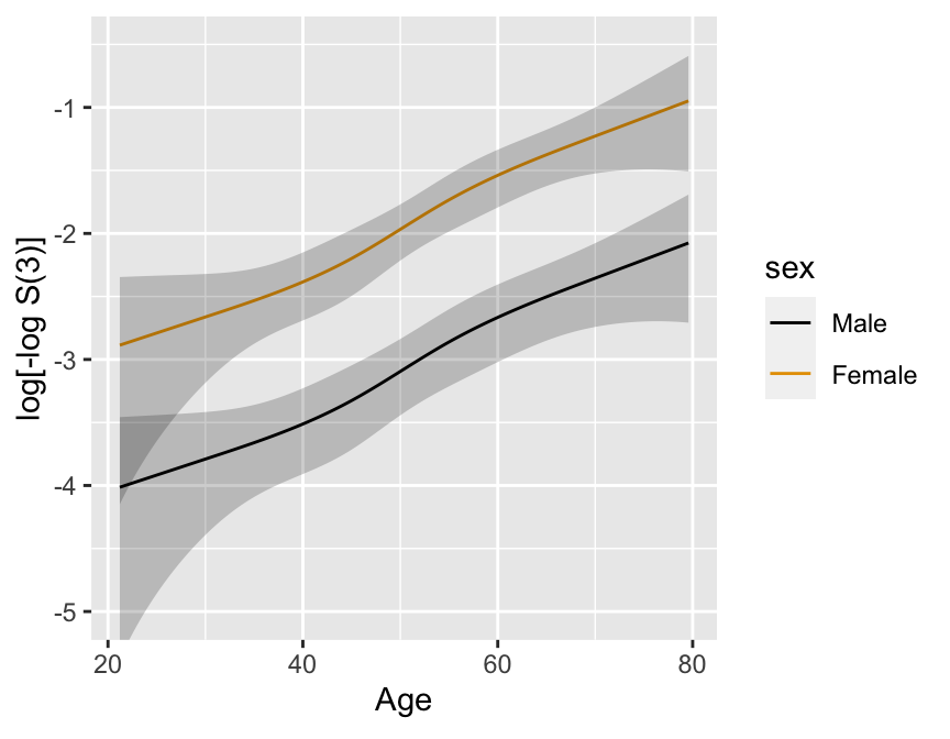
Better:
A 4-knot spline Cox PH model
in two variables ($X_{1}, X_{2}$) which assumes linearity in $X_{1}$ and no $X_{1} \times X_{2}$ interaction
\begin{array}{ccc}
\lambda(t|X) &=& \lambda(t) \exp(\beta_{1}X_{1}+\beta_{2}X_{2}+\beta_{3}X_{2}'+\beta_{4}X_{2}''), \nonumber \\
&=& \lambda(t) \exp(\beta_{1}X_{1}+f(X_{2})),
\end{array}
$$f(X_{2})= \beta_{2}X_{2}+\beta_{3}X_{2}'+\beta_{4}X_{2}''$$
$$\log \lambda(t|X) = \log \lambda(t)+\beta_{1}X_{1}+f(X_{2})$$
To not assume PH in $X_1$, stratify on it:
\begin{array}{ccc}
\log \lambda(t|X_{2},C=j) &=& \log \lambda_{j}(t)+\beta_{1}X_{2}+\beta_{2}X_{2}'+\beta_{3}X_{2}''\nonumber \\
&=& \log \lambda_{j}(t)+f(X_{2})
\end{array}
```{r}
f.noia <- cph(Srv ~ rcs(age,4) + strat(sex), x=TRUE, y=TRUE)
latex(f.noia)
anova(f.noia)
```
```{r}
#| fig.cap: 'Cox PH model stratified on sex, using spline function for age, no interaction. 0.95 confidence limits also shown.'
#| fig.scap: 'Cox PH model stratified on sex, using spline function for age'
#| fig.width: 4.5
#| fig.height: 3.5
#| label: fig-cox-spline-age-sex-noia
# Get accurate C.L. for any age by specifying x=TRUE y=TRUE
# Note: for evaluating shape of regression, we would not
# ordinarily bother to get 3-year survival probabilities -
# would just use X * beta
# We do so here to use same scale as nonparametric estimates
p <- Predict(f.noia, age, sex, time=3, loglog=TRUE)
ggplot(p, ylim=c(-5, -.5))
```
Formal test of linearity: $H_{0}: \beta_{2}=\beta_{3}=0, \chi^{2} =
4.84$, 2 d.f., $P=0.09$.
* Model allowing interaction with sex strata:
\begin{array}{ccc}
\log \lambda(t|X_{2},C=j) &=& \log \lambda_{j}(t)+\beta_{1}X_{2} \\
&+& \beta_{2}X_{2}'+\beta_{3}X_{2}'' \nonumber \\
&+& \beta_{4}X_{1}X_{2}+\beta_{5}X_{1}X_{2}'+\beta_{6}X_{1}X_{2}''
\end{array}
Test for interaction: $P=0.33$.
```{r}
f.ia <- cph(Srv ~ rcs(age,4) * strat(sex), x=TRUE, y=TRUE,
            surv=TRUE)
latex(f.ia)
anova(f.ia)
```
```{r spline-age-sex-ia,w=4.5,h=3.5,cap='Cox PH model stratified on sex, with interaction between age spline and sex. 0.95 confidence limits are also shown.',scap='Cox PH model stratified on sex,with interaction between age spline and sex'}
#| label: fig-cox-spline-age-sex-ia
p <- Predict(f.ia, age, sex, time=3, loglog=TRUE)
ggplot(p, ylim=c(-5, -.5))
```
* Example of modeling a single continuous variable (left ventricular
ejection fraction), outcome = time to cardiovascular death
\begin{array}{ccc}
{\rm LVEF}' &=& {\rm LVEF}\ \ \ \ {\rm if\ \ LVEF}\leq 0.5, \nonumber \\
&=& 0.5~\ \ \ \ \ \ \ {\rm if\ \ LVEF}>0.5
\end{array}
The AICs for 3, 4, 5, and 6-knots spline fits were respectively 126,
124, 122, and 120.
```{r echo=FALSE,h=3.5}
#| label: fig-cox-ef-spline
#| fig-scap: "Spline estimate of relationship between LVEF and relative log hazard"
#| fig-cap: "Restricted cubic spline estimate of relationship between LVEF relative log hazard from a sample of 979 patients and 198 cardiovascular deaths. Data from the Duke Cardiovascular Disease Databank."
knitr::include_graphics('cox-ef-spline.svg')
```
Smoothed residual plot: Martingale residuals, loess smoother
* One vector of residuals no matter how many covariables
* Unadjusted estimates of regression shape obtained by
fixing $\hat{\beta}=0$ for all $X$s
```{r echo=FALSE,h=3.5}
#| label: fig-cox-ef-martingale
#| fig-scap: "Smoothed martingale residuals vs. LVEF"
#| fig-cap: "Three smoothed estimates relating martingale residuals [@the90mar] to LVEF."
knitr::include_graphics('cox-ef-martingale.svg')
```
| Purpose | Method |
|-----|-----|
| Estimate transformation for a single variable | Force $\hat{\beta_{1}}=0$ and compute residuals off of the null regression |
| Check linearity assumption for a single variable | Compute $\hat{\beta_{1}}$ and compute residuals off of the linear regression |
| Estimate marginal transformations for $p$ variables | Force $\hat{\beta_{1}},\ldots,\hat{\beta_{p}}=0$ and compute residuals off the global null model |
| Estimate transformation for variable $i$ adjusted for other $p-1$ variables | Estimate $p-1\ \beta$s, forcing $\hat{\beta_{i}}=0$; compute residuals off of mixed global/null model |
: Uses of martingale residuals for estimating predictor transformations
### Proportional Hazards Assumption {#sec-cox-ph}
* Parallelism of $\log \Lambda$ plots
* Comparison of stratified and modeled estimates of $S(t)$
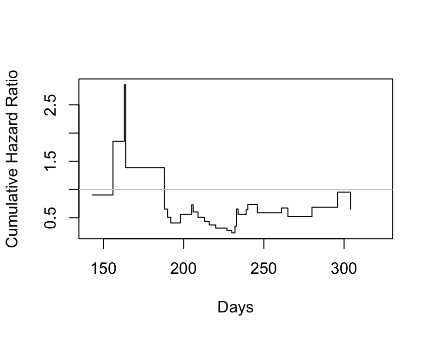
* Plot actual ratio of estimated $\Lambda$, or get differences
in $\log \Lambda$
* Plot $\hat{\Lambda}$ vs. cumulative number of events as $t
\uparrow$
* Stratify time, get interval-specific Cox regression
coefficients: <br>
In an interval, exclude all subjects with <br>
event/censoring time
before start of interval <br>
Censor all events at end of interval
```{r kprats-cumhaz-ratio,w=4.5,h=3.5,cap='Estimate of $\\Lambda_{2}/\\Lambda_{1}$ based on $-\\log$ of Altschuler--Nelson--Fleming--Harrington nonparametric survival estimates.',scap='$\\Lambda$ ratio plot'}
#| label: fig-cox-kprats-cumhaz-ratio
f <- cph(S ~ strat(group), surv=TRUE)
# For both strata, eval. S(t) at combined set of death times
times <- sort(unique(days[death == 1]))
est   <- survest(f, data.frame(group=levels(group)),
                 times=times, conf.type="none")$surv
cumhaz  <- - log(est)
plot(times, cumhaz[2,] / cumhaz[1,], xlab="Days",
     ylab="Cumulative Hazard Ratio", type="s")
abline(h=1, col=gray(.80))
```
| Time Interval | Observations | Deaths | Log Hazard Ratio | Standard Error |
|-----|-----|-----|-----|-----|
| [0,209) |40 |12 |-0.47 |0.59 |
| [209,234) |27 |12 |-0.72 |0.58 |
| 234+ |14 |12 |-0.50 |0.64 |
Overall Cox $\hat{\beta} = -0.57$.
* VA Lung Cancer dataset, squamous vs. (small, adeno)
```{r valung-ratios,eval=FALSE}
getHdata(valung)
with(valung, {
  hazard.ratio.plot(1 * (cell == 'Squamous'), Surv(t, dead),
                    e=25, subset=cell != 'Large',
                    pr=TRUE, pl=FALSE)
  hazard.ratio.plot(1 * kps, Surv(t, dead), e=25,
                    pr=TRUE, pl=FALSE) })
```
| Time Interval |Observations|Deaths| Log Hazard Ratio | Standard Error |
|-----|-----|-----|-----|-----|
| [0,21) | 110 | 26 |-0.46 |0.47 |
| [21,52) | 84 | 26 |-0.90 |0.50 |
| [52,118) | 59 | 26 |-1.35 |0.50 |
| 118+ | 28 | 26 |-1.04 |0.45 |
Estimates for Karnofsky performance status weight over time:
| Time Interval |Observations|Deaths| Log Hazard Ratio | Standard Error |
|-----|-----|-----|-----|-----|
| [0,19]|137 |27 |-0.053 |0.010 |
| [19,49)|112 |26 |-0.047 |0.009 |
| [49,99)|85 |27 |-0.036 |0.012 |
| 99+|28 |26 |-0.012 |0.014 |
```{r echo=FALSE,h=3.5}
#| label: fig-cox-pi-hazard-ratio
#| fig-scap: "Stratified hazard ratios for pain/ischemia index over time"
#| fig-cap: "Stratified hazard ratios for pain/ischemia index over time. Data from the Duke Cardiovascular Disease Databank."
knitr::include_graphics('cox-pi-hazard-ratio.svg')
```
* Schoenfeld residuals computed at each unique failure time
* Partial derivative of $\log L$ with respect to each $X$ in turn
* Grambsch and Therneau scale to yield estimates of $\beta(t)$
* Can form a powerful test of PH
$$\hat{\beta} + dR\hat{V}$$
```{r echo=FALSE,h=3.5}
#| label: fig-cox-pi-schoenfeld
#| fig-scap: "Smoothed Schoenfeld residuals"
#| fig-cap: "Smoothed weighted [@gra94pro] @sch82par residuals for the same data in @fig-cox-pi-hazard-ratio. Test for PH based on the correlation ($\\rho$) between the individual weighted Schoenfeld residuals and the rank of failure time yielded $\\rho=-0.23, z=-6.73, P=2\\times 10^{-11}$."
knitr::include_graphics('cox-pi-schoenfeld.svg')
```
* Can test PH by testing $t \times X$ interaction using time-
dependent covariables
* Separate parametric fits, e.g. Weibull with differing
$\gamma$; hazard ratio is
$$\frac{\alpha\gamma t^{\gamma-1}}{\delta\theta t^{\theta-1}} = \frac{\alpha\gamma}{\delta\theta} t^{\gamma-\theta}$$
| t | log Hazard Ratio |
|-----|-----|
| 10 |-0.36 |
| 36 |-0.64 |
| 83.5 |-0.83 |
| 200 |-1.02 |
* Interaction between $X$ and spline function of $t$:
$$\log \lambda(t|X) = \log\lambda(t) + \beta_{1}X + \beta_{2}Xt + \beta_{3}Xt' + \beta_{4}Xt''$$
The $X+1:X$ log hazard ratio function is estimated by
$$\hat{\beta_{1}} + \hat{\beta_{2}}t + \hat{\beta_{3}}t' + \hat{\beta_{4}}t''$$
```{r echo=FALSE}
v1 <- 'Response Variable $T$<br>Time Until Event'
a1 <- 'Shape of $\\lambda(t|X)$ for fixed $X$ as $t \\uparrow$'
ve1 <- 'Shape of $S_{\\rm KM}(t)$'
v2 <- 'Interaction between $X$ and $T$'
a2 <- 'Proportional hazards -- effect of $X$ does not depend on $T$, e.g. treatment effect is constant over time.'
ve2 <- '• Categorical $X$: check parallelism of stratified $\\log[-\\log S(t)]$ plots as $t \\uparrow$<br>• @mue83com cum. hazard ratio plots<br>@arj88gra cum. hazard plots<br>• Check agreement of stratified and modeled estimates<br>• Hazard ratio plots<br>• Smoothed Schoenfeld residual plots and correlation test (time vs. residual)<br>• Test time-dependent covariable such as $X \\times \\log(t+1)$<br>• Ratio of parametrically estimated $\\lambda(t)$'
v3 <- 'Individual Predictors $X$'
a3 <- 'Shape of $\\lambda(t|X)$ for fixed $t$ as $X \\uparrow$<br>Linear: $\\log \\lambda(t|X)=\\log \\lambda(t)+\\beta X$<br>Nonlinear: $\\log \\lambda(t|X)=\\log \\lambda(t)+f(X)$'
ve3 <- '• $k$-level ordinal $X$ : linear term + $k-2$ dummy variables<br>• Continuous $X$: Polynomials, spline functions, smoothed martingale residual plots'
v4 <- 'Interaction between $X_{1}$ and $X_{2}$'
a4 <- 'Additive effects: effect of $X_{1}$ on $\\log \\lambda$ is independent of $X_{2}$ and vice-versa'
ve4 <- 'Test non-additive terms, e.g. products'
```
| Variables | Assumptions | Verification |
|-----------|-------------|--------------|
| `r v1` | `r a1` | `r ve1` |
| `r v2` | `r a2` | `r ve2` |
| `r v3` | `r a3` | `r ve3` |
| `r v4` | `r a4` | `r ve4` |
: Assumptions of the proportional hazards model
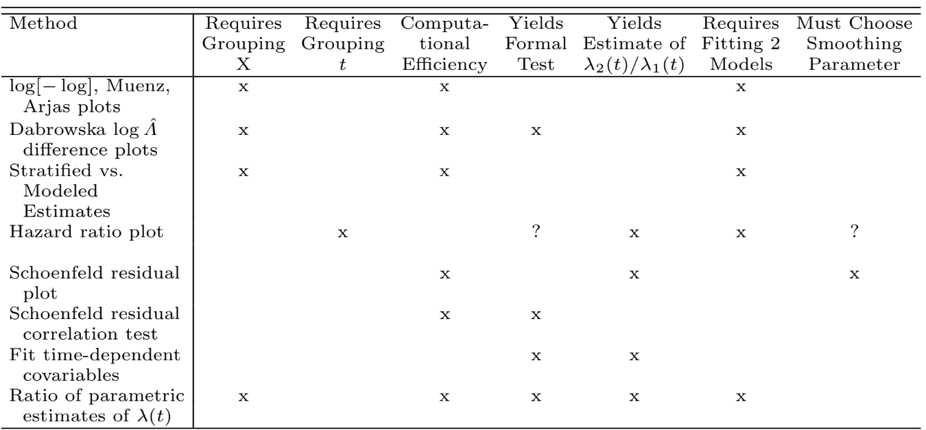
```{r echo=FALSE,out.width='100%'}
#| fig-cap: "Comparison of methods for checking the proportional hazards assumption and for allowing for non-proportional hazards"
knitr::include_graphics('images/cox-method-tab.png')
```
## What to Do When PH Fails
* Test of association not needed and the key variable is categorical $\rightarrow$ stratify
* Key results display: covariate-adjusted cumulative incidence curves by strata with confidence bands for the difference in the two curves
+ allows curves to cross
* $P$-value for testing variable may still be useful
(conservative)
* Survival estimates wrong in certain time intervals
* Can model non-PH:
$$\lambda(t | X) = \lambda_{0}(t) \exp(\beta_{1} X + \beta_{2} X \times \log(t+1))$$
For this model, @bre84two derived a simple 2 d.f. score test for whether one group has a different hazard rate than the other group at any time $t$
* Can also use time intervals:
$$\lambda(t | X) = \lambda_{0}(t) \exp(\beta_{1} X + \beta_{2} X \times [t > c])$$
* Or fit one model for early follow-up, one for late
* Try another model, e.g. log-normal, log-logistic can have effects of $X$ changing constantly over time on the hazard scale
* Example the fit of various link functions in an ordinal model, as this process spans a whole spectrum of PH to AFT models (@sec-ordsurv)
* Differences in mean restricted life length can be useful
in comparing therapies when PH fails [@kar97use], but see [bit.ly/datamethods-rmst](http://datamethods.org/t/restricted-mean-survival-time-and-comparing-treatments-under-non-proportional-hazards/2686)
See @put05lon, @per06red, @mug10fle
## Collinearity
## Overly Influential Observations {#sec-cox-influence}
## Quantifying Predictive Ability {#sec-cox-quant-pred}
\begin{array}{ccc}
R^{2}_{\rm LR}&=& 1 - \exp(-{\rm LR}/n) \nonumber \\
&=& 1 - \omega^{2/n}
\end{array}
* $\omega$ = null model likelihood divided by the fitted model
likelihood
* Divide by max attainable value to get $R_{\rm N}^{2}$
* 4 versions of Maddala-Cox-Snell $R^2$: [hbiostat.org/bib/r2.html](https://hbiostat.org/bib/r2.html)
$c$: concordance probability (between predicted and observed)
* All possible pairs of subjects whose ordering of failure times
can be determined
* Fraction of these for which $X$ ordered same as $Y$
* Somers' $D_{xy} = 2(c-0.5)$
See [fharrell.com/post/addvalue](http://fharrell.com/post/addvalue) for more about the most sensitive values for assessing predictive discrimination and comparing competing models.
## Validating the Fitted Model {#sec-cox-validate}
Separate bootstrap validations for calibration and for discrimination.
For external validation, a sample containing at least 200 events is
needed [@col16sam].
### Validation of Model Calibration {#sec-cox-rel-val}
* Calibration at fixed $t$
* Get $\hat{S}(t | X)$ for all subjects
* Divide into intervals each containing say 50 subjects
* Compare mean predicted survival with K-M
* Bootstrap this process to add back optimism in difference of
these 2, due to overfitting
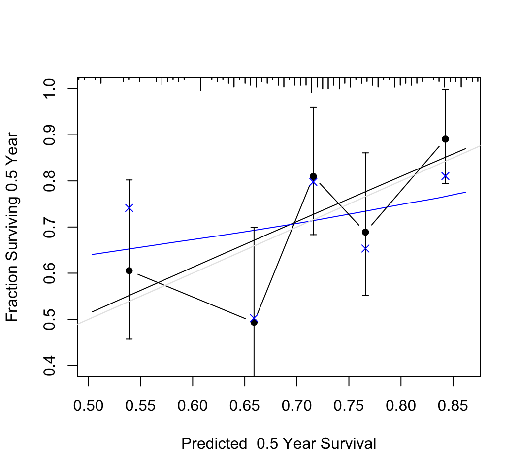
* Ex: 20 random predictors, $n=200$
```{r rel-random,w=5.5,h=5,cap="Calibration of random predictions using Efron's bootstrap with B=200 resamples. Dataset has n=200, 100 uncensored observations, 20 random predictors, model $\\chi^{2}_{20} = 19$. The smooth black line is the apparent calibration estimated by adaptive linear spline hazard regression [@koo95haz], and the blue line is the bootstrap bias-- (overfitting--) corrected calibration curve estimated also by hazard regression. The gray scale line is the line of identity representing perfect calibration. Black dots represent apparent calibration accuracy obtained by stratifiying into intervals of predicted 0.5y survival containing 40 events per interval and plotting the mean predicted value within the interval against the stratum's Kaplan-Meier estimate. The blue $\\times$ represent bootstrap bias-corrected Kaplan-Meier estimates.",scap='Bootstrap calibration of random survival predictions'}
#| label: fig-cox-rel-random
n <- 200
p <-  20
set.seed(6)
xx <- matrix(rnorm(n * p), nrow=n, ncol=p)
y  <- runif(n)
units(y) <- "Year"
e   <- c(rep(0, n / 2), rep(1, n / 2))
f   <- cph(Surv(y, e) ~ xx, x=TRUE, y=TRUE,
           time.inc=.5, surv=TRUE)
cal <- calibrate(f, u=.5, B=200)
par(mar=c(6, 3.5, 1, 1))
plot(cal, ylim=c(.2, 1))#, subtitles=FALSE)
calkm <- calibrate(f, u=.5, m=40,  cmethod='KM', B=200)
plot(calkm, add=TRUE)
```
### Validation of Discrimination and Other Statistical Indexes {#sec-cox-discrim-val}
Validate slope calibration (estimate shrinkage from overfitting):
$$\lambda(t|X) = \lambda(t) \exp(\gamma Xb)$$
```{r val-random}
print(validate(f, B=200), digits=3,
      caption='Bootstrap validation of a Cox model with random predictors')
```
## Describing the Fitted Model
* Can use coefficients if linear and additive
* Can use e.g. inter-quartile-range hazard ratios for
various levels of interacting factors if linearity holds approximately
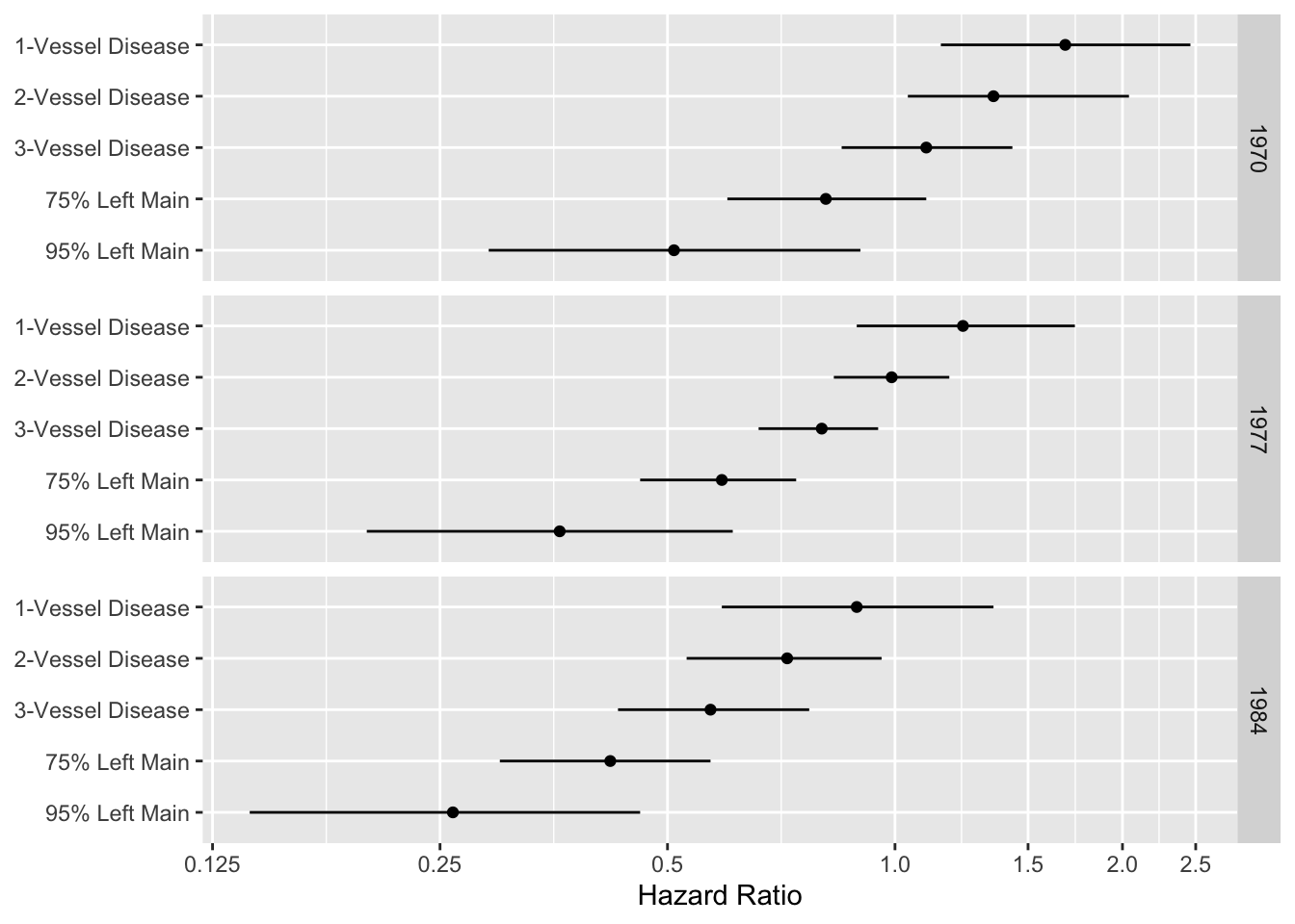
```{r echo=FALSE,out.width='80%'}
#| label: fig-cox-cabg-hazard-ratio
#| fig-scap: "Display of an interactions among treatment, extent of disease, and year"
#| fig-cap: "A display of an interaction between treatment and extent of disease, and between treatment and calendar year of start of treatment. Comparison of medical and surgical average hazard ratios for patients treated in 1970, 1977, and 1984 according to coronary artery disease severity. Circles represent point estimates; bars represent 0.95 confidence limits for hazard ratios. Hazard ratios <1 indicate that surgery is more effective [@cal89evo]."
d <- expand.grid(Disease=c('1-Vessel Disease','2-Vessel Disease',
'3-Vessel Disease', '75% Left Main', '95% Left Main'),
Year=c(1970, 1977, 1984))
d$hr <- c(1.68,1.35,1.10,.81,.51,1.23,.99,.80,.59,.36,.89,.72,.57,.42,.26)
d$low <- c(1.15,1.04,.85,.60,.29,.89,.83,.66,.46,.20,.59,.53,.43,.30,.14)
d$high <- c(2.46,2.04,1.43,1.10,.90,1.73,1.18,.95,.74,.61,1.35,.96,.77,.57,.46)
d$Disease <- factor(d$Disease, levels=rev(levels(d$Disease)))
ggplot(d, aes(x=hr, y=Disease)) + geom_point() + facet_grid(Year ~ .) +
geom_errorbarh(aes(xmin=low, xmax=high, height=0)) +
xlab('Hazard Ratio') + ylab(NULL) +
scale_x_log10(breaks=c(.125,.25,.5,1,1.5,2,2.5),
labels=c('0.125','0.25','0.5','1.0','1.5','2.0','2.5'))
```
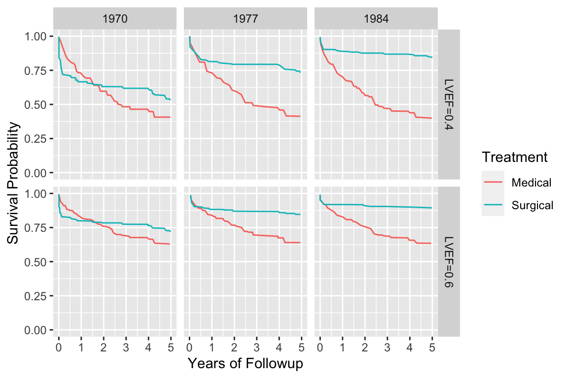
```{r echo=FALSE, w=6, h=4}
#| label: fig-cox-cabg-ef
#| fig-scap: "Cox--Kalbfleisch--Prentice survival estimates stratifying on treatment and adjusting for several predictors"
#| fig-cap: "Cox--Kalbfleisch--Prentice survival estimates stratifying on treatment and adjusting for several predictors, showing a secular trend in the efficacy of coronary artery bypass surgery. Estimates are for patients with left main disease and normal (LVEF=0.6) or impaired (LVEF=0.4) ventricular function [@pry87cha]."
d <- readRDS('cox-cabg-ef.rds')
for(tr in levels(d$Treatment)) {
for(ef in c(.4, .6)) {
for(y in c(1970,1977,1984)) {
cat(y, ef, tr, ' ')
w <- subset(d, Year==y & Treatment==tr & EF==ef)
cat(nrow(w), '\n')
}}}
d$ef <- paste('LVEF', d$EF, sep='=')
ggplot(d, aes(x=t, y=surv, color=Treatment)) + geom_line() +
facet_grid(ef ~ Year) + ylim(0,1) + ylab('Survival Probability') +
xlab('Years of Followup')
```
```{r echo=FALSE,h=2.75}
#| label: fig-cox-tmscore
#| fig-scap: "Cox model predictions with respect to a continuous variable"
#| fig-cap: "Cox model predictions with respect to a continuous variable. $X$-axis shows the range of the treadmill score seen in clinical practice and $Y$-axis shows the corresponding 5-year survival probability predicted by the Cox regression model for the 2842 study patients [@mar87exe]."
knitr::include_graphics('cox-tmscore.svg')
```
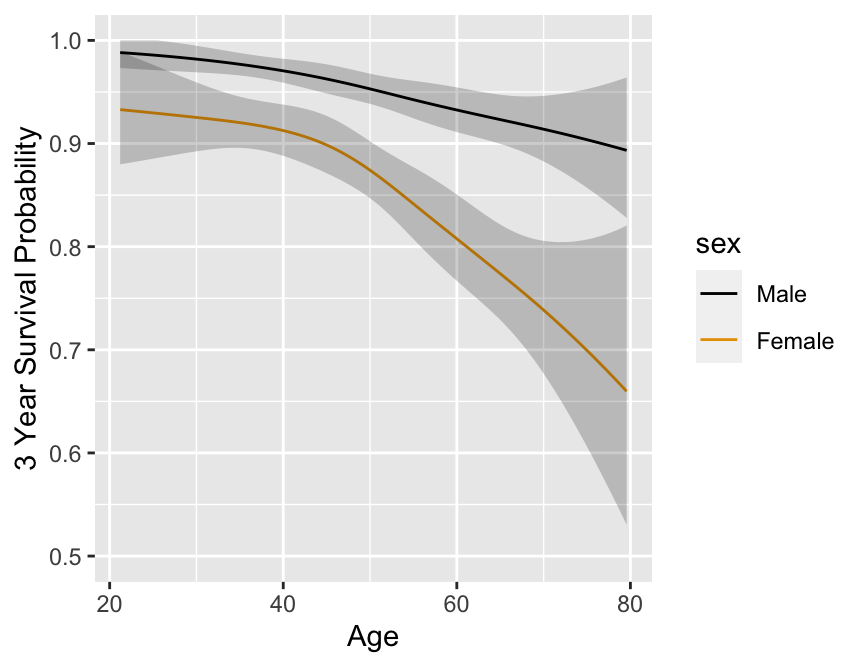
```{r spline-age-sex-ia-surv,w=4.5,h=3.5,cap='Survival estimates for model stratified on sex, with interaction.'}
#| label: fig-cox-spline-age-sex-ia-surv
p <- Predict(f.ia, age, sex, time=3)
ggplot(p)
```
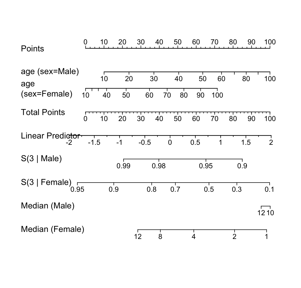
* Nomogram to compute $X\hat{\beta}$
* Also $\hat{S}(t | X)$ for a few $t$
* Can have axis for median failure time if sample is high risk
## `R` Functions {#sec-cox-r}
### Power and Sample Size Calculations, Hmisc Package
* `cpower`: computes power for a two-sample Cox test with
random patient entry over a fixed duration and a given length of
minimum follow-up, using exponential distribution with handling
of dropout and drop-in [@lac86eva]
* `ciapower`: computes power of the Cox
interaction test in a $2 \times 2$ setup using the method of @pet93sam
* `spower`: simulates power for 2-sample tests (the
log-rank test by default)
allowing for very complex conditions such as continuously varying
treatment effect and non-compliance probabilities.
### Cox Model using `rms` Package
* `cph`: slight modification of Therneau's `survival` package
`coxph` function
* `print` method prints the Nagelkerke index $R^{2}_{\rm N}$ (@sec-cox-quant-pred) and up to 4 adjusted and unadjusted Maddala-Cox-Snell $R^2$
* `cph` works with generic functions such as `specs`, `predict`, `summary`, `anova`, `fastbw`, `which.influence`, `latex`, `residuals`, `coef`, `nomogram`, `plot`, `ggplot`, `plotp`. `plot`, `ggplot`, `plotp` have an additional argument `time` for plotting `cph` fits. It also has an argument `loglog` which if `T` causes instead log -log survival to be plotted on the $y$-axis.
* `Survival.cph`, `Quantile.cph`, `Mean.cph`
create other `R` functions to evaluate survival probabilities,
survival time quantiles, and mean and mean restricted lifetimes,
based on a `cph` fit with `surv=TRUE`
* `Quantile` and `Mean` are especially useful with `plot`, `ggplot`, `plotp` and `nomogram`. `Survival` is useful with `nomogram`
* Usually better: use `orm` (@sec-ordsurv) to do Cox regression and more
```{r coxexcode, eval=FALSE}
f <- cph(..., surv=T)
med <- Quantile(f)
plot(nomogram(f, fun=function(x) med(lp=x),
         funlabel='Median Survival Time'))
# fun tranforms the linear predictors
srv <- Survival(f)
rmean <- Mean(f, tmax=3, method='approx')
plot(nomogram(f, fun=list(function(x) srv(3, x), rmean),
         funlabel=c('3-Year Survival Prob.','Restricted Mean')))
# med, srv, expected are more complicated if strata are present
```
The `R` program below demonstrates how several `cph`-related functions
work well with the `nomogram` function to display this last fit.
Here predicted 3-year
survival probabilities and median survival time (when defined) are
displayed against age and sex. The fact that a nonlinear effect
interacts with a stratified factor is taken into account.
```{r spline-age-sex-ia-nomogram,w=6,h=5.75,cap='Nomogram from a fitted stratified Cox model that allowed for interaction between age and sex, and nonlinearity in age. The axis for median survival time is truncated on the left where the median is beyond the last follow-up time.',scap='Nomogram for stratified Cox model'}
#| label: fig-cox-spline-age-sex-ia-nomogram
surv    <- Survival(f.ia)
surv.f  <- function(lp) surv(3, lp, stratum='sex=Female')
surv.m  <- function(lp) surv(3, lp, stratum='sex=Male')
quant   <- Quantile(f.ia)
med.f   <- function(lp) quant(.5, lp, stratum='sex=Female')
med.m   <- function(lp) quant(.5, lp, stratum='sex=Male')
at.surv <- c(.01, .05, seq(.1,.9,by=.1), .95, .98, .99, .999)
at.med  <- c(0, .5, 1, 1.5, seq(2, 14, by=2))
n <- nomogram(f.ia, fun=list(surv.m, surv.f, med.m,med.f),
         funlabel=c('S(3 | Male)','S(3 | Female)',
                    'Median (Male)','Median (Female)'),
         fun.at=list(c(.8,.9,.95,.98,.99),
                     c(.1,.3,.5,.7,.8,.9,.95,.98),
                     c(8,10,12),c(1,2,4,8,12)))
plot(n, col.grid=FALSE, lmgp=.2)
```
```{r}
latex(f.ia, digits=3)
```
```{r echo=FALSE}
saveCap('20')
```