```{r include=FALSE}
require(Hmisc)
options(qproject='rms', prType='html')
require(qreport)
getRs('qbookfun.r')
hookaddcap()
knitr::set_alias(w = 'fig.width', h = 'fig.height', cap = 'fig.cap', scap ='fig.scap')
```
# Case Study in Cox Regression {#sec-coxcase}
Note that all the analyses presented here may be done in a more general context - see @sec-ordsurv
## Choosing the Number of Parameters and Fitting the Model
`r mrg(sound("cox-case-1"))`
* Clinical trial of estrogen for prostate cancer
* Response is time to death, all causes
* Base analysis on Cox proportional hazards model [@cox72reg]
* $S(t | X)$ = probability of surviving at least to time $t$ given set of predictor values $X$
* $S(t | X) = S_{0}(t)^{\exp(X\beta)}$
* Censor time to death at time of last follow-up for patients
still alive at end of study (treat survival time for pt.\
censored at 24m as 24m+)
* Use simple, partial approaches to data reduction
* Use `transcan` for single imputation
* Again combine last 2 categories for `ekg,pf`
* See if we can use a full additive model (4 knots for continuous $X$)
`r ipacue()`
| Predictor | Name | d.f. | Original Levels |
|---|---|---|---|
Dose of estrogen | `rx` | 3 | placebo, 0.2, 1.0, 5.0 mg estrogen |
Age in years | `age` | 3 | |
Weight index: wt(kg)-ht(cm)+200 | `wt` | 3 | |
Performance rating | `pf` | 2 | normal, in bed <50% of time, in bed >50%, in bed always |
History of cardiovascular disease | `hx` | 1 |present/absent |
Systolic blood pressure/10 | `sbp` | 3 | |
Diastolic blood pressure/10 | `dbp` | 3 | |
Electrocardiogram code | `ekg` | 5 | normal, benign, rhythm disturb., block, strain, old myocardial infarction, new MI |
Serum hemoglobin (g/100ml) | `hg` | 3 | |
Tumor size (cm$^2$) | `sz` | 3 | |
Stage/histologic grade combination | `sg` | 3 | |
Serum prostatic acid phosphatase | `ap` | 3 | |
Bone metastasis | `bm` | 1 | present/absent |
* Total of 36 candidate d.f.
* Impute missings and estimate shrinkage `r ipacue()`
```{r}
require(rms)
options(prType='html')    # for print, summary, anova, validate
getHdata(prostate)
levels(prostate$ekg)[levels(prostate$ekg) %in%
                     c('old MI','recent MI')] <- 'MI'
# combines last 2 levels and uses a new name, MI

prostate$pf.coded <- as.integer(prostate$pf)
# save original pf, re-code to 1-4
levels(prostate$pf)  <- c(levels(prostate$pf)[1:3],
                          levels(prostate$pf)[3])
# combine last 2 levels

w <- transcan(~ sz + sg + ap + sbp + dbp + age +
              wt + hg + ekg + pf + bm + hx,
              imputed=TRUE, data=prostate, pl=FALSE, pr=FALSE)

attach(prostate)
sz  <- impute(w, sz, data=prostate)
sg  <- impute(w, sg, data=prostate)
age <- impute(w, age,data=prostate)
wt  <- impute(w, wt, data=prostate)
ekg <- impute(w, ekg,data=prostate)

dd <- datadist(prostate)
options(datadist='dd')

units(dtime) <- 'Month'
S <- Surv(dtime, status!='alive')

f <- cph(S ~ rx + rcs(age,4) + rcs(wt,4) + pf + hx +
         rcs(sbp,4) + rcs(dbp,4) + ekg + rcs(hg,4) +
         rcs(sg,4) + rcs(sz,4) + rcs(log(ap),4) + bm)
print(f, coefs=FALSE)
```
* Global LR $\chi^2$ is 135 and very significant $\rightarrow$
modeling warranted `r ipacue()`
* AIC on $\chi^2$ scale = $136.2 - 2 \times 36 = 64.2$
* Rough shrinkage: 0.74 ($\frac{136.2 - 36}{136.2}$)
* Informal data reduction (increase for `ap`) `r ipacue()`
| Variables | Reductions | d.f. Saved |
|-----------|------------|------------|
| `wt` | Assume variable not important enough for 4 knots; use 3 | 1 |
| `pf` | Assume linearity | 1 |
| `hx,ekg` | Make new 0,1,2 variable and assume linearity: 2=`hx` and `ekg` not normal or benign, 1=either, 0=none | 5 |
| `sbp,dbp` | Combine into mean arterial bp and use 3 knots: map=$\frac{2}{3}$ `dbp` $+ \frac{1}{3}$ `sbp` | 4 |
| `sg` | Use 3 knots | 1 |
| `sz` | Use 3 knots | 1 |
| `ap` | Look at shape of effect of `ap` in detail, and take log before expanding as spline to achieve stability: add 1 knot | -1 |
: Data reduction strategy
```{r}
heart <- hx + ekg %nin% c('normal','benign')
label(heart) <- 'Heart Disease Code'
map   <- (2*dbp + sbp)/3
label(map) <- 'Mean Arterial Pressure/10'
dd <- datadist(dd, heart, map)

f <- cph(S ~ rx + rcs(age,4) + rcs(wt,3) + pf.coded +
         heart + rcs(map,3) + rcs(hg,4) +
         rcs(sg,3) + rcs(sz,3) + rcs(log(ap),5) + bm,
         x=TRUE, y=TRUE, surv=TRUE, time.inc=5*12)
print(f, coefs=FALSE)
# x, y for anova LR, predict, validate, calibrate;
# surv, time.inc for calibrate
anova(f, test='LR')
```
* Savings of 12 d.f. `r ipacue()`
* AIC=70, shrinkage 0.80
## Checking Proportional Hazards {#sec-coxcase-check-ph}
`r mrg(sound("cox-case-2"))`
* This is our tentative model
* Examine distributional assumptions using scaled Schoenfeld residuals
* Complication arising from predictors using multiple d.f.
* Transform to 1 d.f. empirically using $X\hat{\beta}$
* `cox.zph` does this automatically
* Following analysis approx. since internal coefficients estimated
```{r }
z <- predict(f, type='terms')
# required x=T above to store design matrix
f.short <- cph(S ~ z, x=TRUE, y=TRUE)
# store raw x, y so can get residuals
```
* Fit `f.short` has same LR $\chi^2$ of 118 as the fit `f`, `r ipacue()` but with falsely low d.f.
* All $\beta=1$
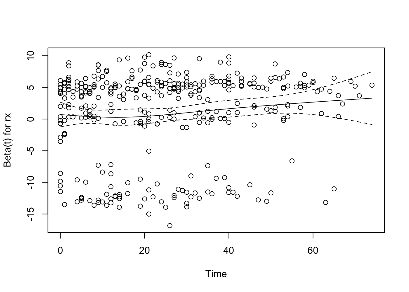
```{r rx-ph,cap='Raw and spline-smoothed scaled Schoenfeld residuals for dose of estrogen, nonlinearly coded from the Cox model fit, with $\\pm$ 2 standard errors.',scap='Schoenfeld residuals for dose of estrogen in Cox model'}
#| label: fig-coxcase-rx-ph
require(survival)   # or use survival::cox.zph(...)
phtest <- cox.zph(f, transform='identity')
phtest
plot(phtest[1]) # plot only the first variable
```
* None of the effects significantly change over time
* Global test of PH $P=0.52$
## Testing Interactions
`r mrg(sound("cox-case-3"))`
* Will ignore non-PH for dose even though it makes sense
* More accurate predictions could be obtained using stratification
or time dep. cov.
* Test all interactions with dose <br> Reduce to 1 d.f. as before
```{r}
z.dose <- z[,"rx"]  # same as saying z[,1] - get first column
z.other <- z[,-1]   # all but the first column of z
f.ia <- cph(S ~ z.dose * z.other, x=TRUE, y=TRUE)
anova(f.ia, test='LR')
```
## Describing Predictor Effects
`r ipacue()`
* Plot relationship between each predictor and $\log \lambda$
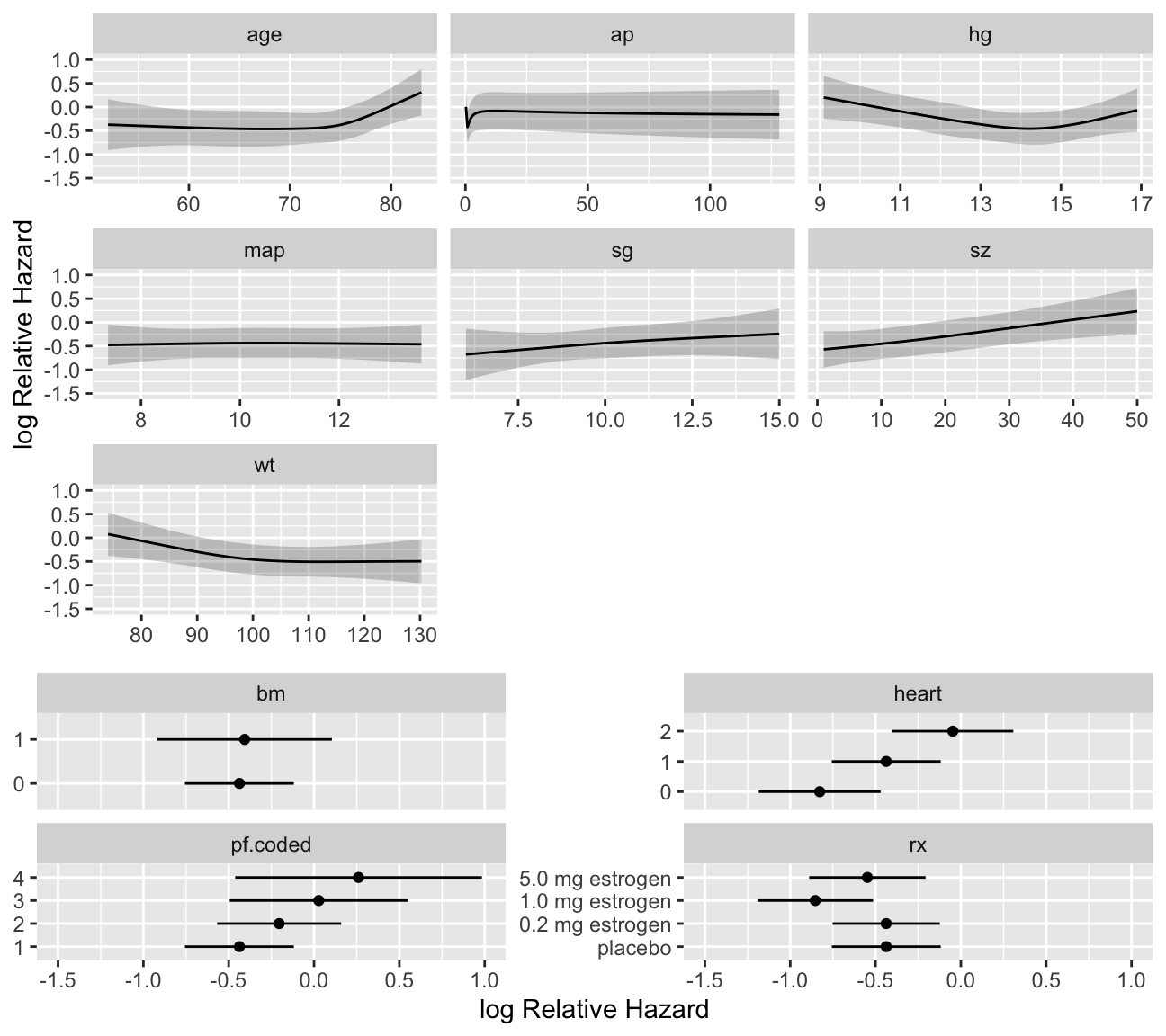
```{r cox-shapes,h=6,w=6.75,cap='Shape of each predictor on log hazard of death. $Y$-axis shows $X\\hat{\\beta}$, but the predictors not plotted are set to reference values. Note the highly non-monotonic relationship with `ap`, and the increased slope after age 70 which has been found in outcome models for various diseases.',scap='Shapes of predictors for log hazard in prostate cancer'}
#| label: fig-coxcase-shapes
ggplot(Predict(f), sepdiscrete='vertical', nlevels=4,
       vnames='names')
```
## Validating the Model
`r ipacue()`
* Validate for $D_{xy}$ and slope shrinkage
```{r}
set.seed(1)  # so can reproduce results
v <- validate(f, B=300)
v
```
* Shrinkage surprisingly close to heuristic estimate of 0.79
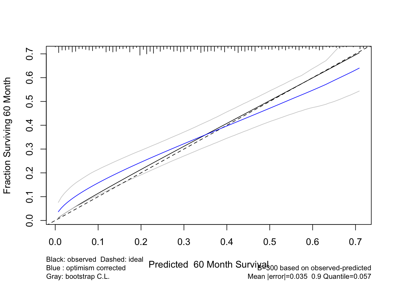
* Now validate 5-year survival probability estimates
```{r cal-cox,cap='Bootstrap estimate of calibration accuracy for 5-year estimates from the final Cox model, using adaptive linear spline hazard regression. Line nearer the ideal line corresponds to apparent predictive accuracy. The blue curve corresponds to bootstrap-corrected estimates.',scap='Bootstrap estimates of calibration accuracy in prostate cancer model'}
#| label: fig-coxcase-cal
cal <- calibrate(f, B=300, u=5*12, maxdim=3)
plot(cal)
```
## Presenting the Model
`r mrg(sound("cox-case-4"))`
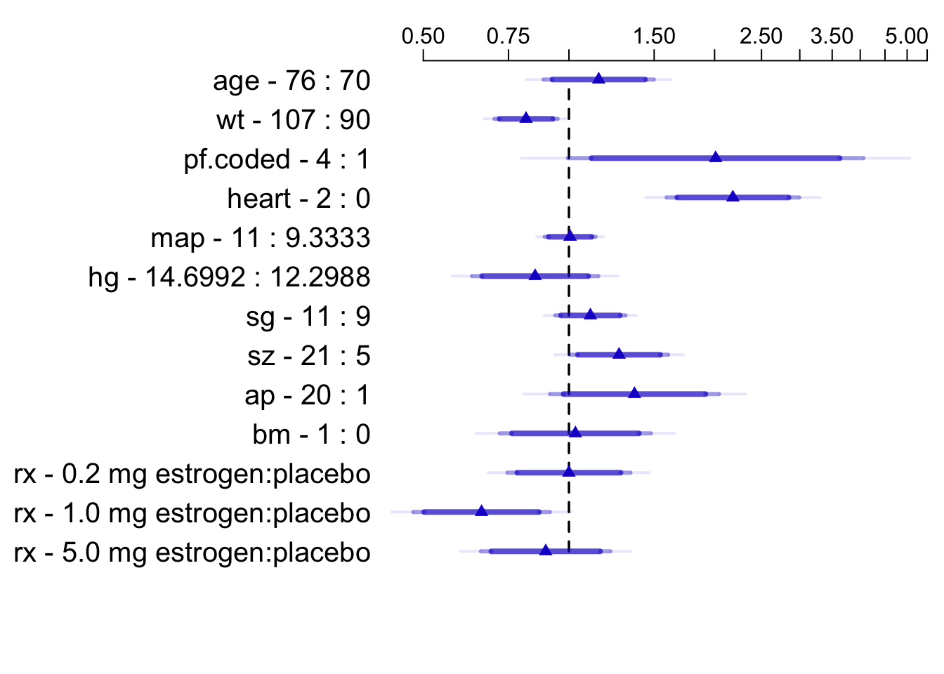
* Display hazard ratios, overriding default for `ap`
```{r summary-cox,cap='Hazard ratios and multi-level confidence bars for effects of predictors in model, using default ranges except for `ap`',scap='Hazard ratios for prostate survival model'}
#| label: fig-coxcase-summary
spar(top=1)
plot(summary(f, ap=c(1,20)), log=TRUE, main='')
```
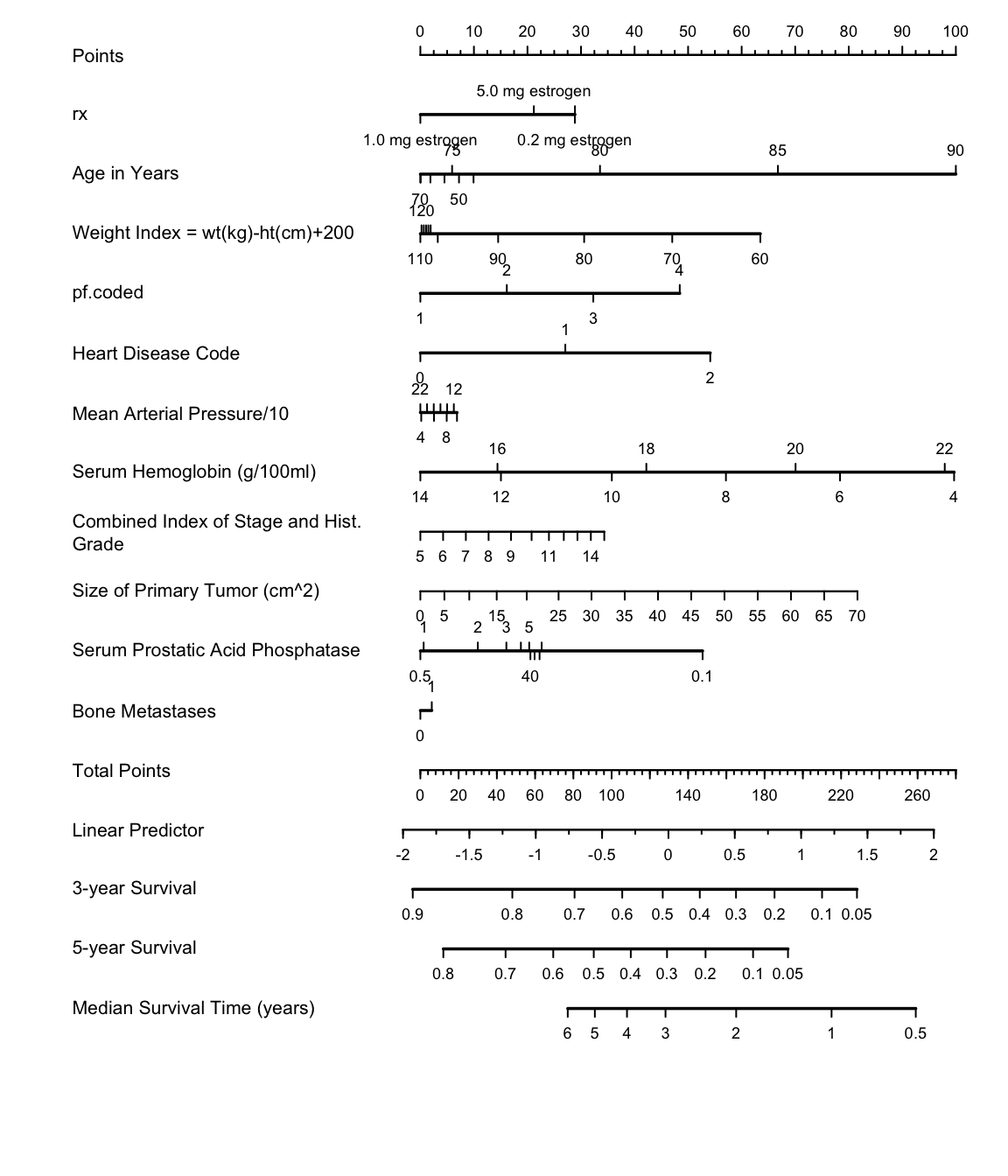
* Draw nomogram, with predictions stated 4 ways
```{r cox-nomogram,w=6,h=7,cap='Nomogram for predicting death in prostate cancer trial'}
#| label: fig-coxcase-nomogram
spar(ps=8)
surv  <- Survival(f)
surv3 <- function(x) surv(3*12,lp=x)
surv5 <- function(x) surv(5*12,lp=x)
quan  <- Quantile(f)
med   <- function(x) quan(lp=x)/12
ss    <- c(.05,.1,.2,.3,.4,.5,.6,.7,.8,.9,.95)

nom <- nomogram(f, ap=c(.1,.5,1,2,3,4,5,10,20,30,40),
                fun=list(surv3, surv5, med),
                funlabel=c('3-year Survival','5-year Survival',
                  'Median Survival Time (years)'),
                fun.at=list(ss, ss, c(.5,1:6)))
plot(nom, xfrac=.65, lmgp=.35)
```
```{r echo=FALSE}
saveCap('21')
```