```{r setup, include=FALSE}
require(Hmisc)
require(qreport)
hookaddcap() # make knitr call a function at the end of each chunk
# to try to automatically add to list of figure
options(prType='html')
getRs('qbookfun.r')
```
`r hypcomment`
`r apacue <- 0`
# Analysis of Covariance in Randomized Studies {#sec-ancova}
`r mrg(ddisc(22))`
<br>
**Big Picture**
* ANCOVA aimed at bringing clarity to contrasts by recognizing within-treatment patient outcome heterogeneity
* Adjustment for baseline imbalance is very secondary and fails to recognize that counter-balancing factors can be found if you keep looking
* In linear models, covariate adjustment $\uparrow$ power
* In nonlinear models, adjustment prevents $\downarrow$ power due to pt heterogeneity
* Classical $2\times 2$ table (e.g. treatment vs. short-term mortality) assumes no within-treatment heterogeneity (e.g., all patients in treatment 1 have probability of death $P_1$)
* Think of cov. adjustment as approximating a design where pt heterogeneity is controlled to the extreme: paired design using identical twins
* **Common criticism**: you left out an important predictor
* **Easy answer**: the unadjusted analysis you proposed left out everything
* A misspecified cov. adjustment performs uniformly better than an unadjusted analysis; poor fit > no fit
**Introduction**
`r mrg(sound("anc-0"))`
* Fundamental clinical question: if I were to give **this patient** treatment B instead of treatment A, by how much should I expect the clinical outcome to be better?
* A gold-standard design is a 6-period 2-treatment randomized crossover study; the patient actually receives both treatments and her responses can be compared
* Using each patient as her own control
* Studies of identical twins come somewhat close to that
* Short of these designs, the best we can do is to ask this fundamental question: <br> If two patients differ at baseline (with respect to available measurements, and on the average with respect to unmeasured covariates) only with regard to assigned treatment, how do their expected outcomes differ?
* Covariate adjustment does that
* Analysis of covariance is classical terminology from linear models but we often use the term also for nonlinear models
* Covariate adjustment means to condition on important facts known about the patients before treatment is given
* We treat baseline values as known constants and do not model their distributions
* Doing a comparison of outcomes that is equalized on baseline characteristics (**within treatment group**) accounts for outcome heterogeneity **within treatment group**
* Accounting for easily accountable (baseline measurements) outcome heterogeneity either
+ maximizes power and precision (in linear models, by reducing residual variance), or
+ gets the model "right" which prevents power loss caused by unexplained outcome heterogeneity (in nonlinear models, by making the model much more correct than assuming identical outcome tendencies for all subjects in a treatment group)
`r mrg(sound("anc-0.1"))`
The model to use depends on the nature of the outcome variable Y, and
different models have different effect measures:
* Continuous Y: we often use difference in means; 2-sample $t$-test assumes all observations in a treatment group have the same mean
+ analyzing heterogeneous $Y$ as if homogeneous (using $t$-test instead of ANCOVA) lowers power and precision by expanding $\sigma^2$, but does not bias the difference in means
* Binary Y: classic $2\times 2$ table assumes every person on treatment T has the same probability of outcome
+ risk difference is only a useful measure in this homogeneous case
+ in heterogeneous case, risk difference will vary greatly, e.g., sicker patients have more "room to move"
+ without covariate adjustment, odds ratios only apply to the homogenous case; in heterogeneous case the unadjusted odds ratio may apply to no one (see
[fharrell.com/post/marg](https://www.fharrell.com/post/marg))
* Time to event: Cox proportional hazards model and its special case the logrank test
+ without covariate adjustment assumes homogeneity within treatment group
+ unadjusted hazard ratio does not estimate a useful quantity if there is heterogeneity
+ non-proportional hazards is more likely without covariate adjustment than with it
- without adjustment the failure time distribution is really a mixture of multiple distributions
<br>
**Hierarchy of Causal Inference for Treatment Efficacy**
`r mrg(sound("anc-0.2"))`
Let $P_{i}$ denote patient $i$ and the treatments be denoted by $A$
and $B$. Thus $P_{2}^{B}$ represents patient 2 on treatment $B$.
$\overline{P}_{1}$ represents the average outcome over a sample of
patients from which patient 1 was selected.
| **Design** | **Patients Compared** |
|-----|-----|
| 6-period crossover | $P_{1}^{A}$ vs $P_{1}^{B}$ (directly measure HTE) |
| 2-period crossover | $P_{1}^{A}$ vs $P_{1}^{B}$ |
| RCT in idential twins | $P_{1}^{A}$ vs $P_{1}^{B}$ |
| $\parallel$ group RCT | $\overline{P}_{1}^{A}$ vs $\overline{P}_{2}^{B}$, $P_{1}=P_{2}$ on avg |
| Observational, good artificial control | $\overline{P}_{1}^{A}$ vs $\overline{P}_{2}^{B}$, $P_{1}=P_{2}$ hopefully on avg |
| Observational, poor artificial control | $\overline{P}_{1}^{A}$ vs $\overline{P}_{2}^{B}$, $P_{1}\neq P_{2}$ on avg |
| Real-world physician practice | $P_{1}^{A}$ vs $P_{2}^{B}$ |
## Covariable Adjustment in Linear Models
`r mrg(sound("anc-1"), disc("ancova-linear"))`
`r quoteit("If you fail to adjust for pre-specified covariates, the statistical model's residuals get larger. Not good for power, but incorporates the uncertainties needed for any possible random baseline imbalances.", 'F Harrell 2019')`
`r ipacue()`
* Model: $E(Y | X) = X \beta + \epsilon$
* Continuous response variable $Y$, normal residuals
* Statistical testing for baseline differences is scientifically incorrect (Altman & Doré 1990, Begg 1990, Senn 1994, Austin et al 2010); as @bla11com stated, statistical tests draw inferences about _populations_, and the population model here would involve a repeat of the randomization to the whole population hence balance would be perfect. Therefore the null hypothesis of no difference in baseline distributions between treatment groups is automatically true.
* If we are worried about baseline imbalance we need to search patient records for counter-- balancing factors
* ⇒ imbalance is not the reason to adjust for covariables
* Adjust to gain efficiency by subtracting explained variation
* Relative efficiency of unadjusted treatment comparison is $1-\rho^2$
* Unadjusted analyses yields unbiased treatment effect estimate
See [here](https://datamethods.org/t/should-we-ignore-covariate-imbalance-and-stop-presenting-a-stratified-table-one-for-randomized-trials)
for a detailed discussion, including reasons not to even stratify by
treatment in "Table 1."
## Covariable Adjustment in Nonlinear Models
`r mrg(sound("anc-2"), disc("ancova-nonlin"))`
<br>
### Hidden Assumptions in $2 \times 2$ Tables
`r ipacue()`
* Traditional presentation of 2--treatment clinical trial with a binary response: $2 \times 2$ table
* Parameters: $P_{1}, P_{2}$ for treatments 1, 2
* Test of goodness of fit: $H_0$: all patients in one treatment group have same probability of positive response ($P_j$ constant)
* ⇒ $H_0$: no risk factors exist
* Need to account for patient heterogeneity
* @mat15inc has a method for estimating the bias in unadjusted the log odds ratio and also has excellent background information
### Models for Binary Response
`r ipacue()`
* Model for probability of event must be nonlinear in predictors unless risk range is tiny
* Useful summary of relative treatment effect is the odds ratio (OR)
* Use of binary logistic model for covariable adjustment will result in an **increase** in the S.E. of the treatment effect (log odds ratio) (@rob91sur)
* But even with perfect balance, adjusted OR $\neq$ unadjusted OR
* Adjusted OR will be farther than 1.0 than unadjusted OR
#### Example from GUSTO--I {#sec-ancova-gusto}
`r mrg(sound("anc-3"), ipacue(marg=FALSE))`
* @ste00cli
* Endpoint: 30--day mortality (0.07 overall)
* 10,348 patients given accelerated $t$--PA
* 20,162 patients given streptokinase (SK)
* Means and Percentages
| Baseline Characteristic | $t$--PA | SK |
|-----|-----|-----|
| Age | 61.0 | 60.9 |
| Female | 25.3 | 25.3 |
| Weight | 79.6 | 79.4 |
| Height | 171.1 | 171.0 |
| Hypertension | 38.2 | 38.1 |
| Diabetes | 14.5 | 15.1 |
| Never smoked | 29.8 | 29.6 |
| High cholesterol| 34.6 | 34.3 |
| Previous MI | 16.9 | 16.5 |
| Hypotension | 8.0 | 8.3 |
| Tachycardia | 32.5 | 32.7 |
| Anterior MI | 38.9 | 38.9 |
| Killip class I | 85.0 | 85.4 |
| ST elevation | 37.3 | 37.8 |
#### Unadjusted / Adj. Logistic Estimates
`r ipacue()`
* With and without adjusting for 17 baseline characteristics
| Type of Analysis | Log OR | S.E. | $\chi^2$ |
|-----|-----|-----|-----|
| Unadjusted | -0.159 | 0.049 | 10.8 |
| Adjusted | -0.198 | 0.053 | 14.0 |
* Percent reduction in odds of death: 15\% vs. 18\
* -0.159 (15\%) is a biased estimate[Some disagree that the word _bias_ is the appropropriate word. This could be called attenuation of the parameter estimate due to an ill-fitting model.]{.aside}
* Increase in S.E. more than offset by increase in treatment effect
* Adjusted comparison based on 19\% fewer patients would have given same power as unadjusted test
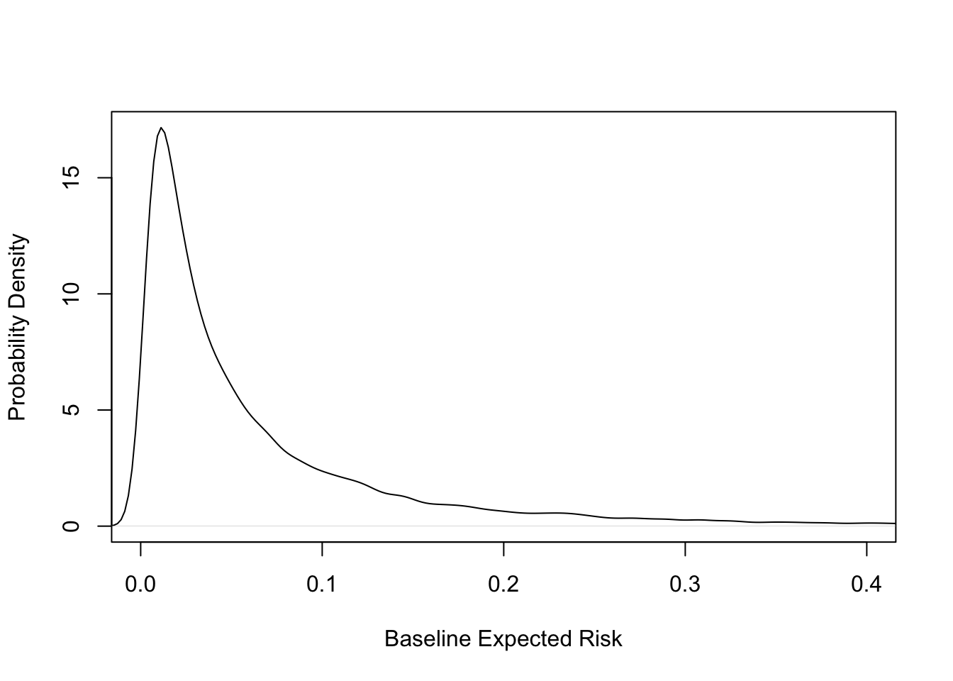
```{r gustohistrisk}
#| label: fig-ancova-gustohistrisk
#| fig-cap: 'Distribution of baseline risk in GUSTO-I. Kernel density estimate of risk distribution for SK treatment. Average risk is 0.07. See also @ioa97imp.'
#| fig-scap: 'Distribution of baseline risk in GUSTO-I'
load('gustomin.rda')
with(gustomin,
     plot(density(p.sk), xlim=c(0, .4), xlab='Baseline Expected Risk',
          ylab='Probability Density', main='') )
```
* See [this](https://www.fharrell.com/post/varyor) for a more in-depth analysis
* Robinson & Jewell: "It is always more efficient to adjust `r ipacue()` for predictive covariates when logistic models are used, and thus in this regard the behavior of logistic regression is the same as that of classic linear regression."
#### Simple Logistic Example -- Gail 1986
| Males | A | B | Total | |
| :------- | ---: | ---: | ------: | --: |
|Y=0 | 500 | 900 | 1400 | |
|Y=1 | 500 | 100 | 600 | |
|Total | 1000| 1000| 2000 | OR=9 |
<br>
|Females|A|B|Total| |
| :--------- | ---: | ---: | -------: | --: |
|Y=0 | 100| 500| 600| |
|Y=1 | 900| 500|1400| |
|Total |1000|1000|2000| OR=9 |
<br>
| Pooled | A | B | Total | |
| :-------- | ---: | ---: | -------: | --: |
|Y=0 |600 | 1400 | 2000 | |
|Y=1 | 1400 | 600 | 2000 | |
|Total | 2000 | 2000 | 4000 | OR=5.44 |
From seeing this example one can argue that odds ratios, like hazard
ratios, were never really designed to be computed on a set of subjects
having heterogeneity in their expected outcomes. See
[fharrell.com/post/marg](https://www.fharrell.com/post/marg) for more.
### Nonlinear Models, General
`r mrg(sound("anc-4"), ipacue(marg=FALSE))`
* @gai84bia showed that for unadjusted treatment estimates to be unbiased, regression must be linear or exponential
* @gai86adj showed that for logistic, Cox, and paired survival models unadjusted treatment effects are asymptotically biased low in absolute value
* Gail also studied normal, exponential, additive risk, Poisson
`r quoteit('Part of the problem with Poisson, proportional hazard and logistic regression approaches is that they use a single parameter, the linear predictor, with no equivalent of the variance parameter in the Normal case. This means that lack of fit impacts on the estimate of the predictor.', '@sen04con, p. 3747')`
## Cox / Log--Rank Test for Time to Event
`r mrg(disc("ancova-efficiency"))`
* Lagakos & Schoenfeld 1984 showed that type I probability is preserved if don't adjust
* If hazards are proportional conditional on covariables, they are not proportional if omit covariables `r ipacue()`
* Morgan 1986 derived asymptotic relative efficiencies (ARE) of unadjusted log--rank test if a binary covariable is omitted
* If prevalence of covariable $X$ is 0.5:
| $X=1 : X=0$ Hazard Ratio | ARE |
|-----|-----|
| 1.0 | 1.00 |
| 1.5 | 0.95 |
| 2.0 | 0.88 |
| 3.0 | 0.72 |
`r ipacue()`
* @for95mod: Treatment effect does not have the same interpretation under unadjusted and adjusted models
* No reason for the two hazard ratios to have the same value
* @aka97pow: Power of unadjusted and stratified log--rank test
| Number | Range of | Power | Power |
|-----|-----|-----|-|
| of Strata | Log Hazards | Unadj. | Adjusted |
| 1 | 0 | .78 | -- |
| 2 | 0--0.5 | .77 | .78 |
| | 0--1 | .67 | .78 |
| | 0--2 | .36 | .77 |
| 4 | 0--3 | .35 | .77 |
| 8 | 0--3.5 | .33 | .77 |
### Sample Size Calculation Issues
* @sch83sam implies that covariable adjustment can only $\uparrow$ sample size in randomized trials `r ipacue()`
* Need to recognize ill--definition of unadjusted hazard ratios
## Why are Adjusted Estimates Right?
`r mrg(sound("anc-5"), disc("ancova-meaning"))`
* @hau98sho, who have an excellent review of covariable adjustment in nonlinear models, state:
`r quoteit('For use in a clinician--patient context, there is only a single person, that patient, of interest. The subject-specific measure then best reflects the risks or benefits for that patient. Gail has noted this previously [ENAR Presidential Invited Address, April 1990], arguing that one goal of a clinical trial ought to be to predict the direction and size of a treatment benefit for a patient with specific covariate values. In contrast, population--averaged estimates of treatment effect compare outcomes in groups of patients. The groups being compared are determined by whatever covariates are included in the model. The treatment effect is then a comparison of average outcomes, where the averaging is over all omitted covariates.', '@hau98sho')`
`r ipacue()`
## How Many Covariables to Use? {#sec-ancova-p}
`r mrg(disc("ancova-plan"))`
* Try to adjust for the bulk of the variation in outcome (@hau98sho,@tuk93tig)
* @neu98est: "to improve the efficiency of estimated covariate effects of interest, analysts of randomized clinical trial data should adjust for covariates that are strongly associated with the outcome" `r ipacue()`
* @raa04how have more guidance for choosing covariables and provide a formula for linear model that shows how the value of adding a covariable depends on the sample size
* Recall that if $R^2$ is an accurate estimate of the large-sample $R^2 \rightarrow$ relative efficiency of unadjusted to adjusted treatment comparison = $1 - R^2$
* For linear models, adding $q$ d.f. for covariates ($q$ covariates if all act linearly) reduces effective same size by $q$
* **But** small increases in $R^2$ more than make up for this in increased efficiency
* Adding pure noise can reduce efficiency
* How much increase in $R^2$ is needed to increase efficient?
* These metrics are approximately equivalent:
+ increase likelihood ratio $\chi^2$ statistic by $> q$ (its expected value under the null for added covariates, i.e., covariates add more than chance in explaining outcome variation)
+ increase $R^{2}_\text{adj}$
+ decrease $\hat{\sigma}^{2}$
* For the last metric: $R^{2} = \frac{SSR}{SST} = 1 - \frac{SSE}{SST}$ where $SST$ is the total sum of squares, $SSR$ is the sum of squares due to regression, and $SSE$ is the sum of squared errors (residuals)
* $\hat{\sigma}^{2} = \frac{SSE}{n - p - 1} = \frac{SST (1 - R_{1}^{2})}{n - p -1}$ for the smaller model with $p$ regression parameters excluding the intercept
* Using $1 - R^{2}_\text{adj} = (1 - R^{2}) \frac{n-1}{n - p - 1}$ we find the ratio of the larger model $\hat{\sigma}^2$ to the small model's is $\frac{1 - R^{2}_\text{adj2}}{1 - R^{2}_\text{adj1}}$ so the residual variance estimate $\downarrow$ if $R^{2}_\text{adj} \uparrow$
* Example: $R^{2}_{1} = 0.3, p = 5, n=150$; increase $R^{2}$ to breakeven $R^2$ of $1 - \frac{143}{144} \times 0.7 = 0.30486$ without sacrificing efficiency by adding $q=1$ covariate
```{r}
ir2 <- function(r21, r22, n, p, q) {
  r2a <- function(r2, n, p) 1 - (1 - r2) * (n - 1) / (n - p - 1)
  cat(' Increase in LR chi-square:', round(-n * log(1 - r22) + n * log(1 - r21), 2), '\n',
      'Adjusted R^2:', round(c(r2a(r21, n, p), r2a(r22, n, p + q)), 3), '\n')
}
ir2(0.3, 0.30486, 150, 5, 1)
```
* Effect when doubling the sample size:
```{r}
ir2(0.3, 0.30486, 300, 5, 1)
```
## Differential and Absolute Treatment Effects {#sec-ancova-txeffects}
### Modeling Differential Treatment Effect
`r mrg(sound("anc-6"), blog("rct-mimic"), disc("ancova-hte"))`
Differential treatment effect is often called _heterogeneity of treatment effect_ or HTE. As opposed to the natural expansion of
absolute treatment effect with underlying subject risk, differential
treatment effect is usually based on analyses of relative effects, especially
when the outcome is binary.
The most common approach to analyzing differential treatment effect
involves searching for such effects rather than estimating the
differential effect. This is, tragically, most often done through
subgroup analysis.
#### Problems With Subgroup Analysis
`r ipacue()`
* Subgroup analysis is widely practiced and widely derided in RCTs (as well as in observational studies)
* Construction of a subgroup from underlying factors that are continuous in nature (e.g., "older" = age $\geq 65$) assumes that the treatment effect is like falling off a cliff, i.e., all-or-nothing. Discontinuous treatment effects, like discontinuous main effects, have not been found and validated but have always been shown to have been an artificial construct driven by opinion and not data.
* Given a subgroup a simple label such as "class IV heart failure" may seem to be meaningful but subgrouping carries along other subject characteristics that are correlated with the subgrouping variable. So the subgroup's treatment effect estimate has a more complex interpretation than what is thought.
* Researchers who don't understand that "absence of evidence is not evidence for absence" interpret a significant effect in one subgroup but not in another as the treatment being effective in the first but ineffective in the second. The second $P$-value may be large because of increased variability in the second subgroup or because of a smaller effective sample size in that group.
* Testing the treatment effect in a subgroup does not carry along with it the covariate adjustment needed and assumes there is no residual HTE _within_ the subgroup.
* When treatment interacts with factors not used in forming the subgroup, or when the subgrouping variable interacts with an ignored patient characteristic, the subgroup treatment effect may be grossly misleading. As an example, in GUSTO-I there was a strong interaction between Killip class and age. Unadjusted analysis of treatment effect within older subjects was partially an analysis of Killip class. And the treatment effect was not "significant" in older patients, leading many readers to conclude $t$--PA should not be given to them. In fact there was no evidence that age interacted with treatment, and the absolute risk reduction due to $t$--PA _increased_ with age.
#### Specifying Interactions
`r mrg(sound("anc-7"), ipacue(marg=FALSE))`
* Assessing differential treatment effect best done with formal interaction tests rather than subgroup analysis
* Pre--specify sensible effect modifiers
+ interactions between treatment and extent of disease
+ "learned" interventions: interaction between treatment and duration of use by physician
* Interactions with center are not necessarily sensible
* Need to use penalized estimation (e.g., interaction effects as random effects) to get sufficient precision of differential treatment effects, if # interaction d.f. $> 4$ for example @sar96hie and @yam99inv
`r ipacue()`
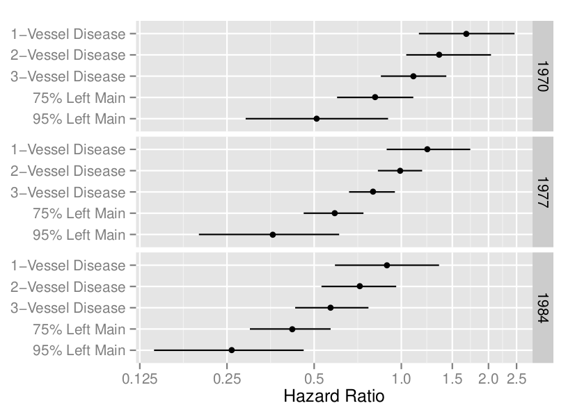
```{r coxcabg, echo=FALSE, out.width="100%", fig.cap="A display of an interaction between treatment, extent of disease, and calendar year of start of treatment (@cal89evo)"}
#| label: fig-ancova-coxcabg
knitr::include_graphics('images/cox-cabg-hazard-ratio.png')
```
#### Strategy for Analyzing Differential Treatment Effect
`r mrg(sound("anc-8"))`
The broad strategy that is recommended is based on the following: `r ipacue()`
* Anything resembling subgroup analysis should be avoided
* Anything that assumes that the treatment effect has a discontinuity in a continuous variable should be avoided. Differential effects should be smooth dose-response effects.
* Anything that results in a finding that has a simpler alternate explanation should be avoided
+ Specify models so that an apparent interaction is not just a stand-in for an omitted main effect
Particulars of the strategy are: `r ipacue()`
* Formulate a subject-matter driven covariate model, including all covariates understood to have strong effects on the outcome. Ensure that these covariates are adjusted for in every HTE analysis context.
* Main effects need to be flexibly modeled (e.g., using regression splines) so as to not assume linearity. False linearity assumptions can inflate apparent interaction effects because the interaction may be co-linear with omitted nonlinear main effects.
* If the sample size allows, also model interaction effects as smooth nonlinear functions. As with main effects, it is not uncommon for interaction effects to be nonlinear, e.g., the effect of treatment is small for age $<70$ then starts to expand rapidly after age 70^[This does not imply that age should be modeled as a categorical variable to estimate the interaction; that would result in unexplained HTE in the age $\geq 70$ interval.]. As a compromise, force interactions to be linear even if main effects are not, if the effective sample size does not permit estimating parameters for nonlinear differential effects.
* Consider effect modifiers that are somewhat uncorrelated with each other. Add the main effects corresponding to each potential effect modifier into the model described in the previous point. For example if the primary analysis uses a model containing age, sex, and severity of disease and one is interested in assessing HTE by race and by geographical region, add _both_ race and region to the main effects that are adjusted for in _all_ later models. This will result in proper covariate adjustment and will handle the case where an apparent interaction is partially explained by an omitted main effect that is co-linear with one of the interacting factors.
* Carry out a joint (chunk) likelihood ratio or $F$-test for all `r ipacue()` potential interaction effects combined. This test has a perfect multiplicity adjustment and will not be "brought down" by the potential interactions being co-linear with each other. The $P$-value from this joint test with multiple degrees of freedom will place the tests described in the next step in context. But note that with many d.f. the test may lack power.
* Consider each potential interaction one-at-a-time by adding that interaction term to the _comprehensive_ main effects model. In the example given above, main effects simultaneously adjusted for would include treatment, age, sex, severity of disease, race, and region. Then treatment $\times$ race is added to the model and tested. Then the race interaction term (but not its main effect) is removed from the model and is replaced by region interactions.
Concerning the last step, we must really recognize that there are two purposes for the analysis of differential treatment effect: `r ipacue()`
1. Understanding which subject characteristics are associated with alterations in efficacy
1. Predicting the efficacy for an individual subject
For the latter purpose, one might include all potential treatment interactions in the statistical model, whether interactions for multiple baseline variables are co-linear or not. Such co-linearities do not hurt predictions or confidence intervals for predictions. For the former purpose, interactions can make one effect modifier compete with another, and neither modifier will be significant when adjusted for the other. As an example, suppose that the model had main effects for treatment, age, sex, and systolic and diastolic blood pressure (SBP, DBP) and we entertained effect modification due to one or both of SBP, DBP. Because of the correlation between SBP and DBP, the main effects for these variables are co-linear and their statistical significance is weakened because they estimate, for example, the effect of increasing SBP holding DBP constant (which is difficult to do). Likewise, treatment $\times$ SBP and treatment $\times$ DBP interactions are co-linear with each other, making statistical tests for interaction have low power. We may find that neither SBP nor DBP interaction is "significant" after adjusting for the other, but that the combined chunk test for SBP or DBP interaction is highly significant. Someone who does not perform the chunk test may falsely conclude that SBP does not modify the treatment effect. This problem is more acute when more than two factors are allowed to interact with treatment.
Note that including interaction terms in the model makes all treatment
effect estimates conditional on specific covariate values, effectively
lowering the sample size for each treatment effect estimate. When
there is no HTE, the overall treatment main effect without having interaction
terms in the model is by far the highest precision estimate. There is
a bias-variance tradeoff when considering HTE. Adding interaction
terms lowers bias but greatly increases variance.
Another way to state the HTE estimation strategy is as follows. `r ipacue()`
1. Pick a model for which it is mathematically possible that there be no interactions (no restrictions on model parameters)
1. Develop a model with ample flexibly-modeled main effects and clinically pre-specified interactions. Use a Bayesian skeptical prior or penalized maximum likelihood estimate to shrink the interaction terms if the effective sample size does not support the pre-specified number of interaction parameters. Be sure to model interaction effects as continuous if they come from variables of an underlying continuous nature.
1. Display and explain relative effects (e.g., odds ratios) as a function of interacting factors and link that to what is known about the mechanism of treatment effect.
1. Put all this in a context (like Figure @fig-ancova-ordiff) that shows absolute treatment benefit (e.g., risk scale) as a function of background risk and of interacting factors.
1. State clearly that background risk comes from all non-treatment factors and is a risk-difference accelerator that would increase risk differences for any risk factor, not just treatment. Possibly provide a risk calculator to estimate background risk to plug into the $x$-axis.
Consider simulated two-treatment clinical trial data to illustrate the "always adjust for all main effects but consider interactions one at a time" approach to analyzing and displaying evidence for differential treatment effec. After that we will illustrate a simultaneous interaction analysis. Simulate time-to-event data from an exponential distribution, and fit Cox proportional hazards models to estimate the interaction between age and treatment and between sex and treatment. The true age effect is simulated as linear in the log hazard and the treatment effect on the log relative hazard scale is proportional to how far above 60 years is a patient's age, with no treatment benefit before age 60. This is a non-simple interaction that could be exactly modeled with a linear spline function, but assume that the analyst does not know the true form of the interaction so she allows for a more general smooth form using a restricted cubic spline function. The data are simulated so that there is no sex interaction.
```{r htesim}
require(rms)
options(prType='html')   # for cph print, anova
set.seed(1)
n <- 3000    # total of 3000 subjects
age <- rnorm(n, 60, 12)
label(age) <- 'Age'
sex   <- factor(sample(c('Male', 'Female'), n, rep=TRUE))
treat <- factor(sample(c('A', 'B'), n, rep=TRUE))
cens  <- 15 * runif(n)     # censoring time
h <- 0.02 * exp(0.04 * (age - 60) + 0.4 * (sex == 'Female') -
                0.04 * (treat == 'B') * pmax(age - 60, 0))
dt <- -log(runif(n)) / h
label(dt) <- 'Time Until Death or Censoring'
e <- ifelse(dt <= cens, 1, 0)
dt <- pmin(dt, cens)
units(dt) <- 'Year'
dd <- datadist(age, sex, treat); options(datadist='dd')
S <- Surv(dt, e)
f <- cph(S ~ sex + rcs(age, 4) * treat)
f
anova(f)
```
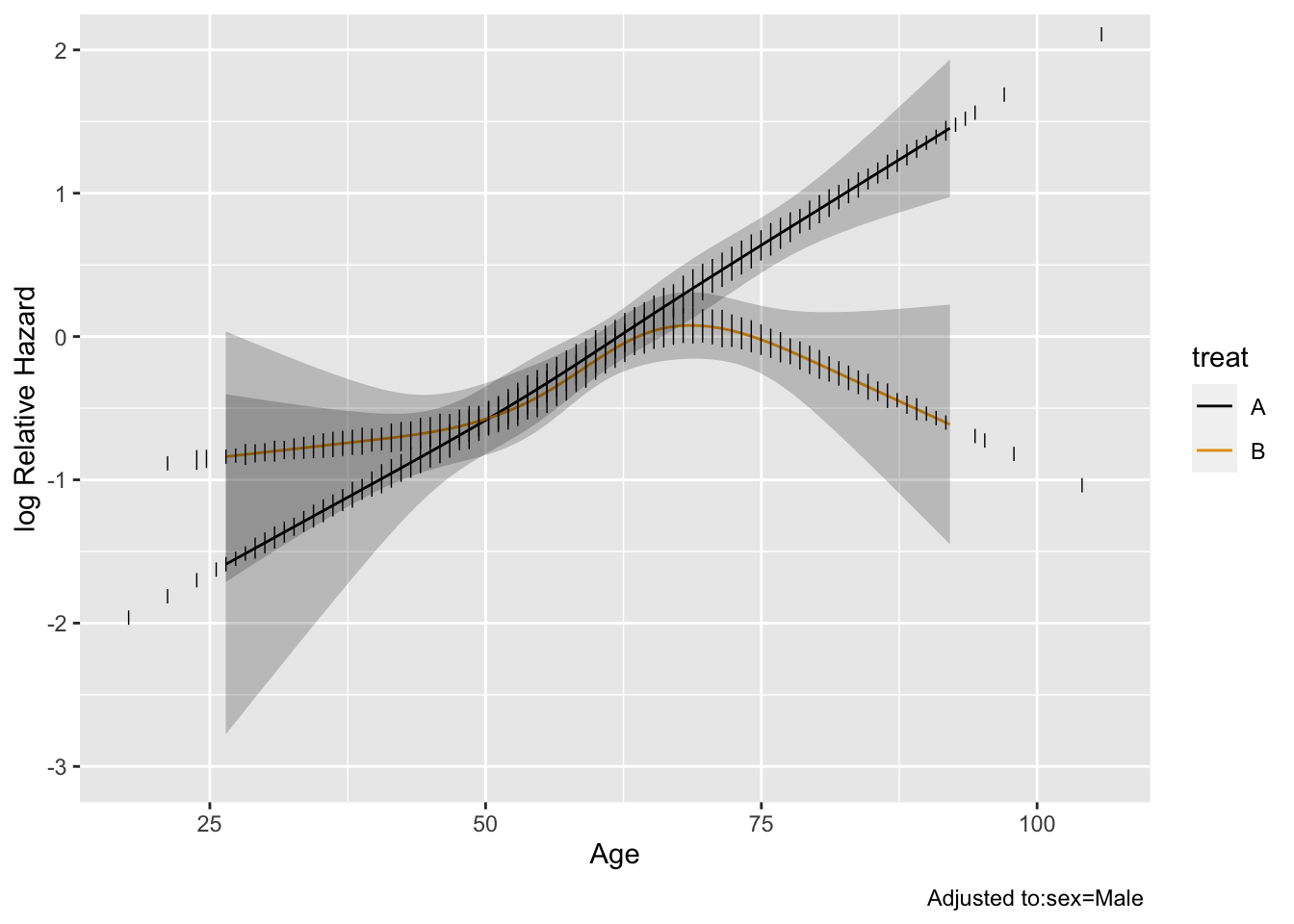
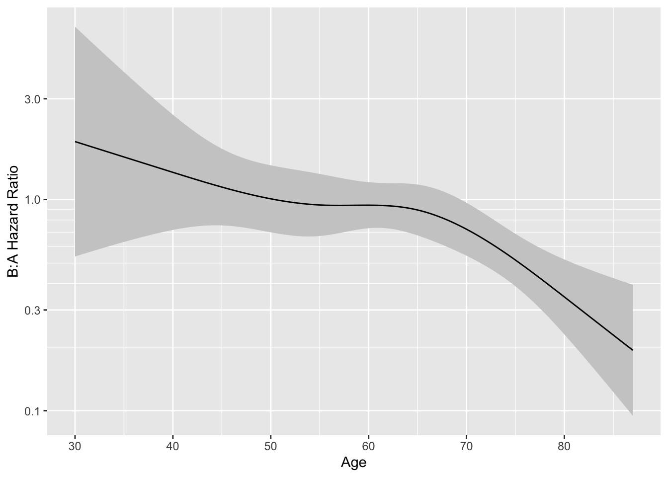
The model fitted above allows for a general age $\times$ treatment interaction. Let's explore this interaction by plotting the age effect separately by treatment group, then plotting the treatment B:A hazard ratio as a function of age.
```{r hteplot}
#| label: fig-ancova-hteplot
#| fig-cap: "Estimates from model with age $\\times$ treatment interaction"
#| fig-subcap:
#| - "Age effect separately by treatment"
#| - "B:A hazard ratio vs. age"
ggplot(Predict(f, age, treat), rdata=data.frame(age, treat))
ages <- seq(30, 87, length=200)
k <- contrast(f, list(treat='B', age=ages), list(treat='A', age=ages))
k <- as.data.frame(k[Cs(sex,age,Contrast,Lower,Upper)])
ggplot(k, aes(x=age, y=exp(Contrast))) +
  scale_y_log10(minor_breaks=seq(.2, .9, by=.1)) +
  geom_ribbon(aes(ymin=exp(Lower), ymax=exp(Upper)), fill='gray80') +
  geom_line() +
  ylab('B:A Hazard Ratio') + xlab('Age')
```
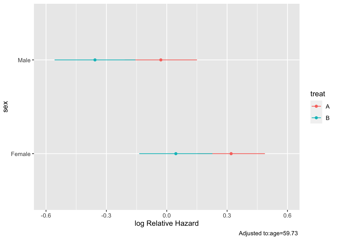
Re-fit the model allowing for a sex interaction (but not an age interaction) and display the results.
```{r hteplot2}
g <- cph(S ~ sex * treat + rcs(age, 4))
g
anova(g)
k <- contrast(g, list(treat='B', sex=levels(sex)), list(treat='A', sex=levels(sex)))
k <- as.data.frame(k[Cs(sex,age,Contrast,Lower,Upper)])
kabl(k)
```
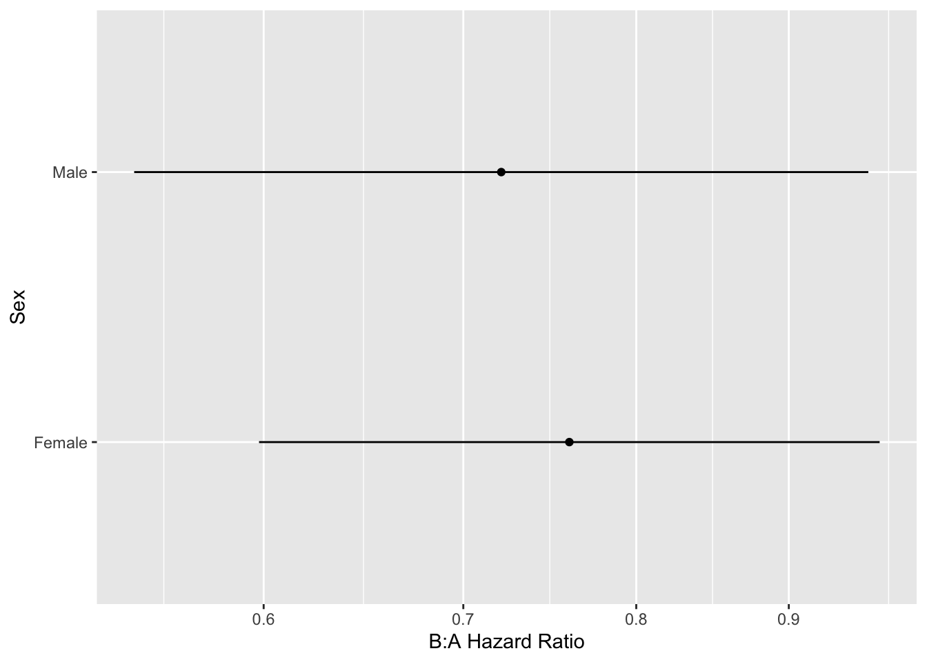
```{r hteplot3}
#| label: fig-ancova-hteplot3
#| fig-cap: "Effects of predictors in Cox model"
#| fig-subcap:
#| - "Partial effects plot"
#| - "B:A hazard ratio by sex"
ggplot(Predict(g, sex, treat))
ggplot(k, aes(y=exp(Contrast), x=sex)) + geom_point() +
  scale_y_log10(breaks=c(.5, .6, .7, .8, .9, 1, 1.1)) +
  geom_linerange(aes(ymin=exp(Lower), ymax=exp(Upper))) +
  xlab('Sex') + ylab('B:A Hazard Ratio') + coord_flip()
```
The above analysis signified a treatment effect for both sex groups (both confidence limits exclude a hazard ratio of 1.0), whereas this should only be the case when age exceeds 60. No sex $\times$ treatment interaction was indicated.
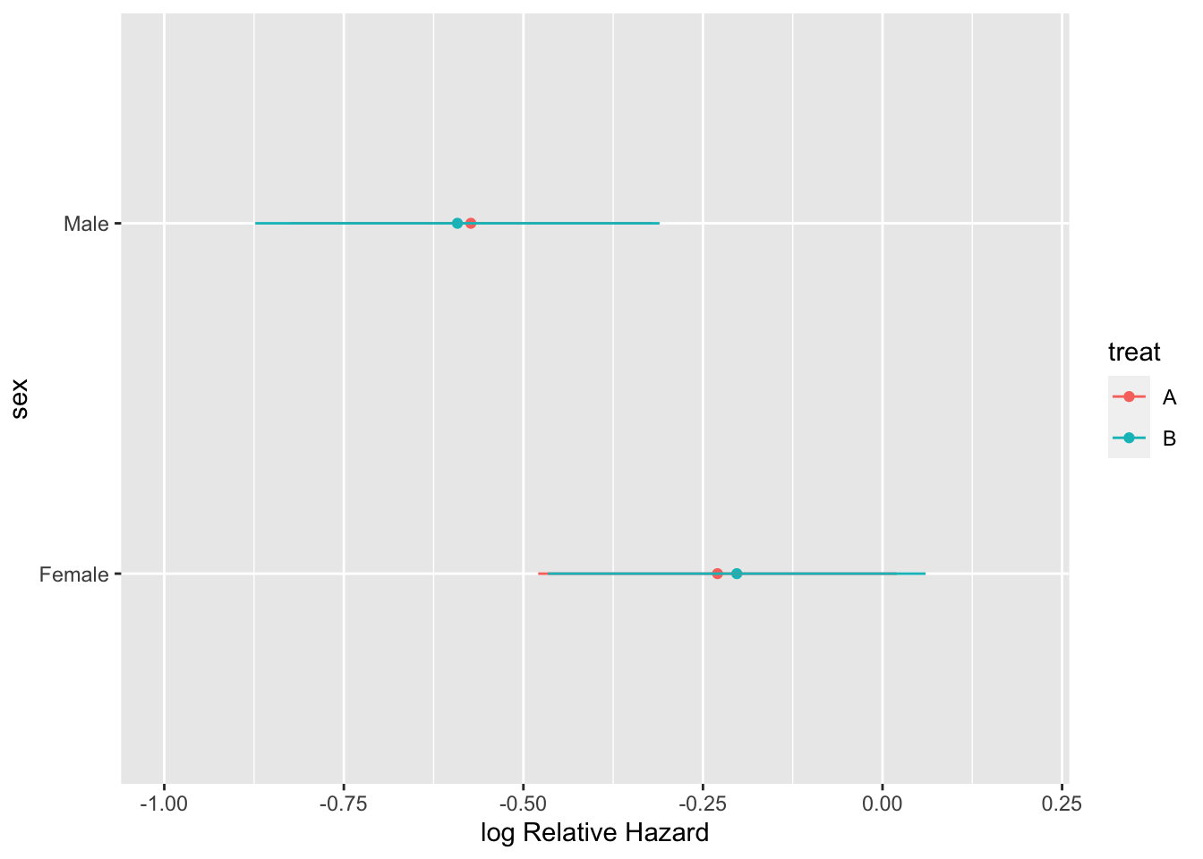
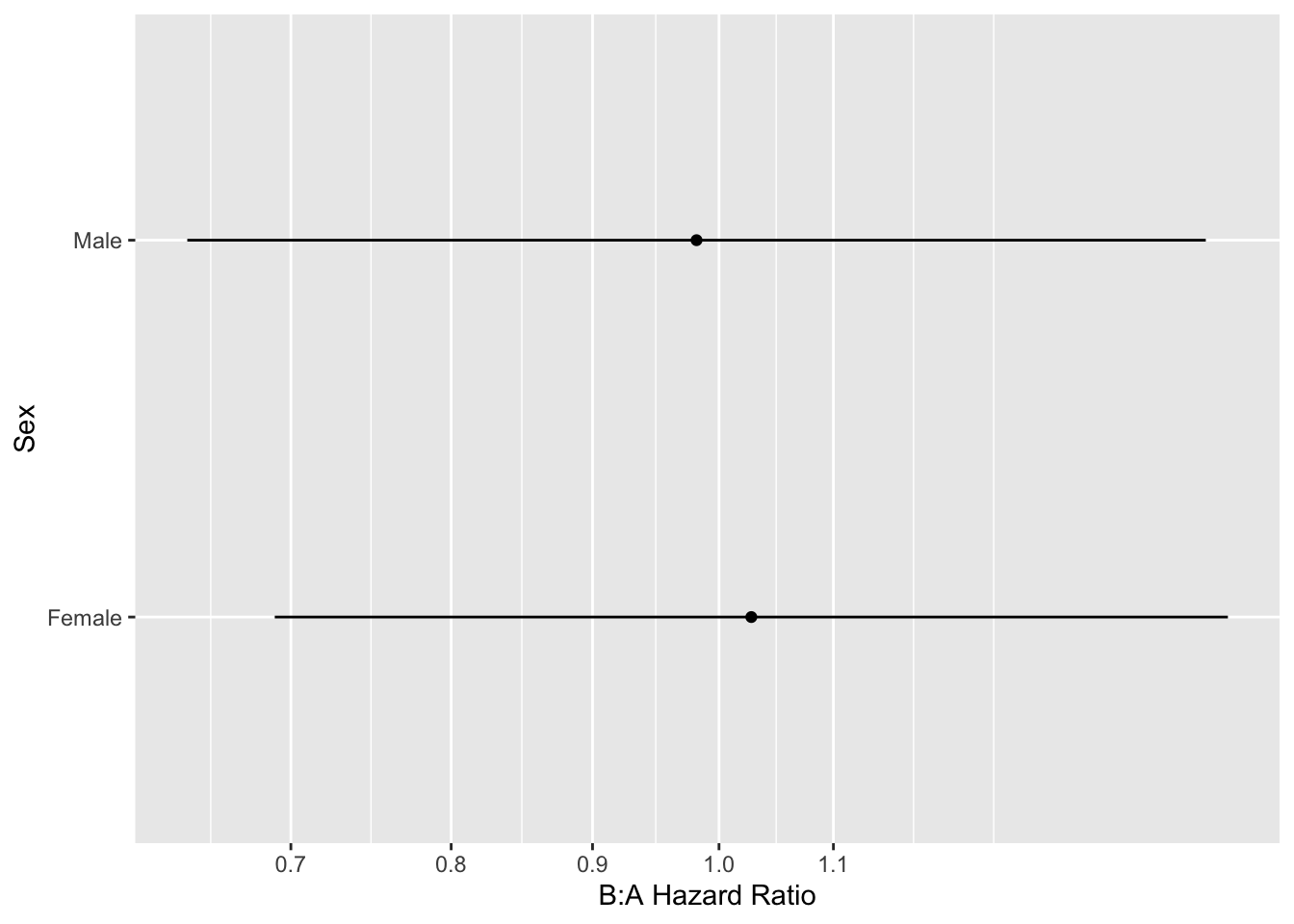
Re-do the previous analysis adjusting for an age $\times$ treatment interaction while estimating the sex $\times$ treatment interaction. For this purpose we must specify an age value when estimating the treatment effects by sex. Here we set age to 50 years. Were age and sex correlated, the joint analysis would have been harder to interpret.
```{r htejointm}
h <- cph(S ~ treat * (rcs(age, 4) + sex))
anova(h)
```
```{r htejoint}
#| label: fig-ancova-htejoint
#| fig-cap: 'Estimates from a Cox model allowing treatment to interact with both age and sex'
#| fig-subcap:
#| - "Partial effects plot"
#| - "B:A hazard ratio by sex age age=50"
ggplot(Predict(h, sex, treat, age=50))
k <- contrast(h, list(treat='B', sex=levels(sex), age=50),
                 list(treat='A', sex=levels(sex), age=50))
k <- as.data.frame(k[Cs(sex,age,Contrast,Lower,Upper)])
ggplot(k, aes(y=exp(Contrast), x=sex)) + geom_point() +
  scale_y_log10(breaks=c(.5, .6, .7, .8, .9, 1, 1.1)) +
  geom_linerange(aes(ymin=exp(Lower), ymax=exp(Upper))) +
  xlab('Sex') + ylab('B:A Hazard Ratio') + coord_flip()
```
This is a more accurate representation of the true underlying model, and is easy to interpret because (1) age and sex are uncorrelated in the simulation model used, and (2) only two interactions were considered.
#### Absolute vs. Relative Treatment Effects Revisited
`r mrg(sound("anc-9"), disc("ancova-absolute"))`
Statistical models are typically chosen so as to maximize the
likelihood of the model fitting the data and processes that generated
them. Even though one may be interested in absolute effects, models
must usually be based on relative effects so that quantities such as
estimated risk are in the legal $[0,1]$ range. It is not unreasonable
to think of a relative effects model such as the logistic model as
providing supporting evidence that an interacting effect _causes_
a change in the treatment effect, whereas the necessary expansion of
treatment effect for higher risk subjects, as detailed in the next
section, is merely a mathematical necessity for how probabilities
work. One could perhaps say that any factor that confers increased
risk for a subject (up to the point of diminishing returns; see below)
might _cause_ an increase in the treatment effect, but this is a
general phenomenon that is spread throughout all risk factors
independently of how they may directly affect the treatment effect.
Because of this, additive risk models are not recommended for modeling
outcomes or estimating differential treatment effects on an absolute
scale. This logic leads to the following recommended strategy: `r ipacue()`
1. Base all inference and predicted risk estimation on a model most likely to fit the data (e.g., logistic risk model; Cox model). Choose the model so that it is _possible_ that there may be no interactions, i.e., a model that does not place a restriction on regression coefficients.
1. Pre-specify sensible possible interactions as described earlier
1. Use estimates from this model to estimate relative differential treatment effects, which should be smooth functions of continuous baseline variables
1. Use the same model to estimate absolute risk differences (as in the next section) as a function both of interacting factors and of baseline variables in the model that do not interact with treatment (but will still expand the absolute treatment effect)
1. Even better: since expansion of risk differences is a general function of overall risk and not of individual risk factors only display effects of individual risk factors that interact with treatment (interacting on the scale that would have allowed them not to interact---the relative scale such as log odds) and show the general risk difference expansion as in Figures @fig-ancova-or-diff (think of the "risk factor" as treatment) and @fig-ancova-gusto-nomogram
`r quoteit('To translate the results of clinical trials into practice may require a lot of work involving modelling and further background information. \'Additive at the point of analysis but relevant at the point of application\' should be the motto.', '[Stephen Senn](http://errorstatistics.com/2013/04/19/stephen-senn-when-relevance-is-irrelevant)')`
### Estimating Absolute Treatment Effects
`r mrg(sound("anc-10"), disc("ancova-absolute"))`
* Absolute efficacy measures:
+ Risk difference ($\delta$)
+ number needed to treat (reciprocal of risk difference) `r ipacue()`
+ Years of life saved
+ Quality--adjusted life years saved
* Binary response, no interactions with treatment, risk for control patient $P$: <br>
$\delta = P - \frac{P}{P + (1-P)/OR}$
* $\delta$ is dominated by $P$ `r ipacue()`
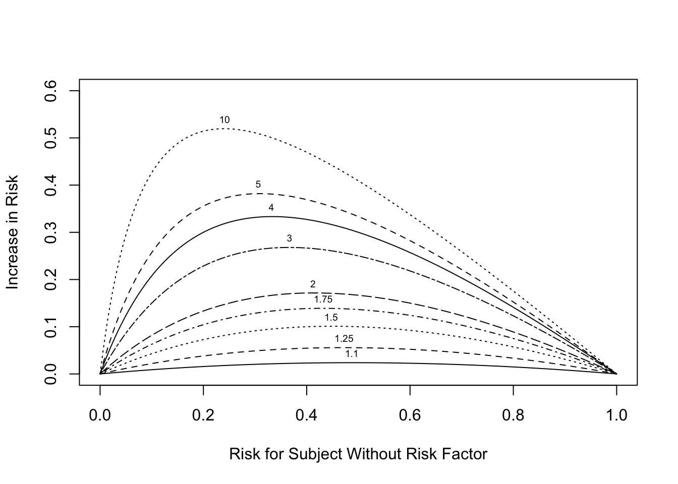
```{r or-diff,w=5.5,h=4,fig.cap='Absolute risk increase as a function of risk for control subject. Numbers on curves are treatment:control odds ratios.',fig.scap='Absolute risk increase as a function of risk'}
#| label: fig-ancova-or-diff
plot(0, 0, type="n", xlab="Risk for Subject Without Risk Factor",
     ylab="Increase in Risk",
     xlim=c(0,1), ylim=c(0,.6))
i <- 0
or <- c(1.1,1.25,1.5,1.75,2,3,4,5,10)
for(h in or) {
  i <- i + 1
  p <- seq(.0001, .9999, length=200)
  logit <- log(p/(1 - p))  # same as qlogis(p)
  logit <- logit + log(h)  # modify by odds ratio
  p2 <- 1/(1 + exp(-logit))# same as plogis(logit)
  d <- p2 - p
  lines(p, d, lty=i)
  maxd <- max(d)
  smax <- p[d==maxd]
  text(smax, maxd + .02, format(h), cex=.6)
}
```
If the outcome is such that $Y=1$ implies a good outcome,
Figure @fig-ancova-or-diff would be useful for estimating the
absolute risk increase for a "good" treatment by selecting the one
curve according to the odds ratio the treatment achieved in a
multivariable risk model. This assumes that the treatment does not
interact with any patient characteristic(s).
@kla15est described the importance of correctly modeling interactions when estimating absolute treatment benefit.
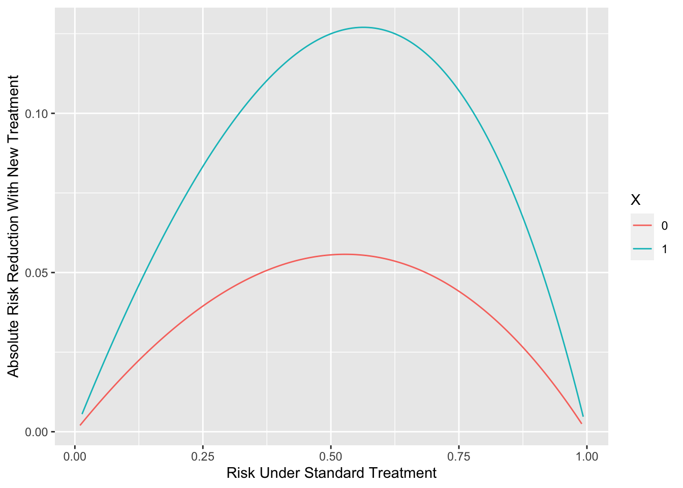
Now consider the case
`r mrg(sound("anc-11"))`
where $Y=1$ is a bad outcome and $Y=0$ is a good outcome, and there is
differential relative treatment effect according to a truly binary
patient characteristic $X=0,1$. Suppose that treatment represents a
new agent and the control group is patients on standard therapy.
Suppose that the new treatment multiplies the odds of a bad outcome by
0.8 when $X=0$ and by 0.6 when $X=1$, and that the background risk
that $Y=1$ for patients on standard therapy ranges from 0.01 to 0.99.
The background risk could come from one or more continuous variables
or mixtures of continuous and categorical patient characteristics.
The "main effect" of $X$ must also be specified. We assume that
$X=0$ goes into the background risk and $X=1$ increases the odds that
$Y=1$ by a factor of 1.4 for patients on standard therapy.
All of this specifies a full probability model that can be evaluated
to show the absolute risk reduction by the new treatment as a function
of background risk and $X$.
`r ipacue()`
```{r ordiff,h=4,w=5.5,fig.cap='Absolute risk reduction by a new treatment as a function of background risk and an interacting factor',fig.scap='Absolute risk reduction by background risk and interacting factor'}
#| label: fig-ancova-ordiff
require(Hmisc)
d <- expand.grid(X=0:1, brisk=seq(0.01, 0.99, length=150))
d <- upData(d,
            risk.standard = plogis(qlogis(brisk) + log(1.4) * X),
            risk.new      = plogis(qlogis(brisk) + log(1.4) * X +
                                     log(0.8) * (X == 0) +
                                     log(0.6) * (X == 1)),
            risk.diff     = risk.standard - risk.new,
            X = factor(X) )
ggplot(d, aes(x=risk.standard, y=risk.diff, color=X)) +
  geom_line() +
  xlab('Risk Under Standard Treatment') +
  ylab('Absolute Risk Reduction With New Treatment')   # (* `r ipacue()` *)
```
It is important to note that the magnification of absolute risk
reduction by increasing background risk should not be labeled (or
analyzed) by any one contributing risk factor. This is a generalized
effect that comes solely from the restriction of probabilities to the
$[0,1]$ range.
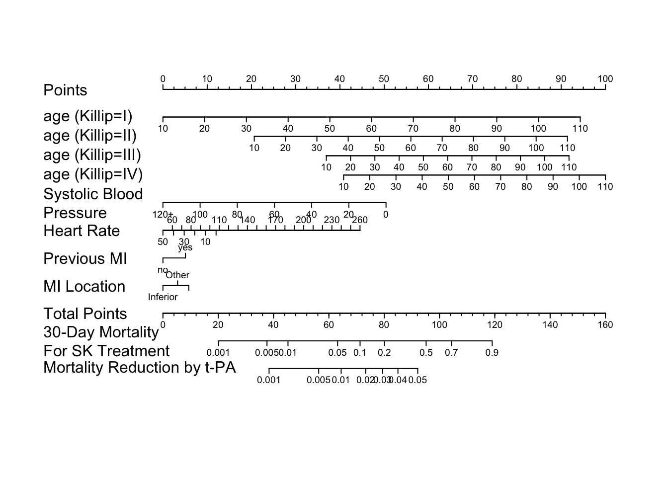
#### Absolute Treatment Effects for GUSTO--I
`r mrg(sound("anc-12"), ipacue(marg=FALSE))`
* [No evidence](https://www.fharrell.com/post/varyor) for interactions with treatment
* Misleading subgroup analysis showed that elderly patients not benefit from $t$--PA; result of strong age $\times$ Killip class interaction
* Wide variation in absolute benefit of $t$--PA
`r ipacue()`
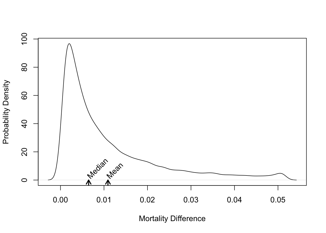
```{r gusto-histdelt,w=5,h=4,fig.cap='Distribution of absolute risk reduction with $t$--PA vs. SK',fig.scap='Absolute benefit vs. baseline risk'}
#| label: fig-ancova-gusto-histdelt
delta <- with(gustomin, p.sk - p.tpa)
plot(density(delta), xlab='Mortality Difference',
     ylab='Probability Density', main='')
m <- mean(delta)
u <- par("usr")
arrows(m, u[3], m, 0, length=.1, lwd=2)
text(m, 2, 'Mean', srt=45, adj=0)
med <- median(delta)
arrows(med, u[3], med, 0, length=.1, lwd=2)
text(med, 2, 'Median', srt=45, adj=0)
```
* Overall mortality difference of 0.011 dominated by high--risk patients
`r ipacue()`
```{r gusto-nom}
load('gusto.rda')
require(rms)
dd <- datadist(gusto); options(datadist='dd')
f <- lrm(day30 ~ tx + age * Killip + pmin(sysbp, 120) +
           lsp(pulse, 50) + pmi + miloc, data=gusto)
cat('<br><small>')
f
anova(f)
cat('</small>')
cof <- coef(f)             # vector of regression coefficients
# For cof, X*beta without treatment coefficients estimates logit
# for SK+t-PA combination therapy (reference cell).  The coefficient for
# SK estimates the difference in logits from combo to SK.  The coefficient
# for tPA estimates the difference in tPA from combo.  The mortality
# difference of interest is mortality with SK minus mortality with tPA.
mort.sk   <- function(x) plogis(x + cof['tx=SK'])
mort.diff <- function(x)
  ifelse(x < 0, mort.sk(x) - plogis(x + cof['tx=tPA']), NA)
# only define when logit < 0 since U-shaped
n <- nomogram(f, fun=list(mort.sk, mort.diff),
              funlabel=c("30-Day Mortality\nFor SK Treatment",
                         "Mortality Reduction by t-PA"),
              fun.at=list(c(.001,.005,.01,.05,.1,.2,.5,.7,.9),
                c(.001,.005,.01,.02,.03,.04,.05)),
              pulse=seq(0,260,by=10), omit='tx', lp=FALSE)
```
```{r gusto-nomogram,fig.cap='Nomogram to predict SK - $t$--PA mortality difference, based on the difference between two binary logistic models.',fig.scap='GUSTO-I nomogram',w=7.5,h=6.5}
#| label: fig-ancova-gusto-nomogram
plot(n, varname.label.sep=' ', xfrac=.27, lmgp=.2, cex.axis=.6)
```
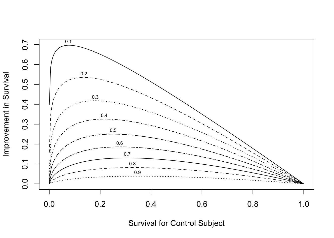
#### Absolute Benefit on Survival Prob.
`r mrg(sound("anc-13"), ipacue(marg=FALSE))`
* Cox PH model
* Modeling can uncover time course of treatment effect
* $X_1$ = treatment, $A={X_{2},\ldots,X_{p}}$ adjustment variables
* Survival difference is <br> $S(t | X_{1}=1, A) - S(t | X_{1}=0, A) = S(t | X_{1}=0, A)^{HR} - S(t | X_{1}=0, A)$
`r ipacue()`
```{r hr-vs-surv,w=5.5,h=4,fig.cap='Relationship between baseline risk, relative treatment effect (hazard ratio --- numbers above curves) and absolute treatment effect.',fig.scap='Baseline risk, hazard ratio, and absolute effect'}
#| label: fig-ancova-hr-vs-surv
plot(0, 0, type="n", xlab="Survival for Control Subject",
     ylab="Improvement in Survival",
     xlim=c(0,1), ylim=c(0,.7))
i <- 0
hr <- seq(.1, .9, by=.1)
for(h in hr) {
  i <- i + 1
  p <- seq(.0001, .9999, length=200)
  p2 <- p ^ h
  d <- p2 - p
  lines(p, d, lty=i)
  maxd <- max(d)
  smax <- p[d==maxd]
  text(smax,maxd+.02, format(h), cex=.6)
}
```
* See also @ken07lim
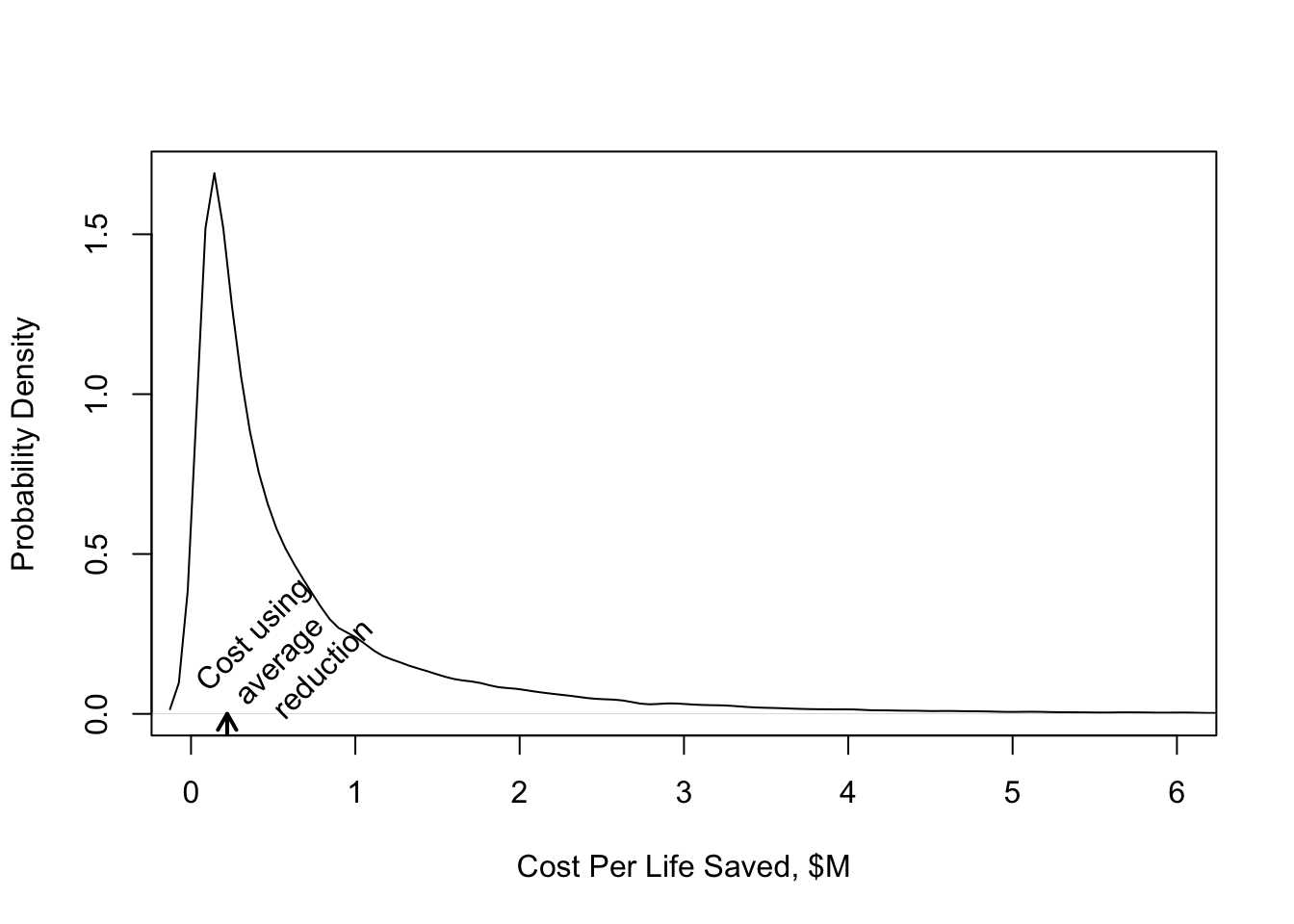
## Cost--Effectiveness Ratios
`r mrg(sound("anc-14"), disc("ancova-ceratio"))`
* Effectiveness E (denominator of C--E ratio) is always absolute
* Absolute treatment effectiveness varies greatly with patient characteristics `r ipacue()`
* ⇒ C--E ratio varies greatly
* A C--E ratio based on average E and average C may not apply to any existing patient!
* Need a model to estimate E
* C may also depend on patient characteristics
`r ipacue()`
```{r gusto-histcost,w=5,h=4,fig.cap='Distribution of cost per life saved in GUSTO--I'}
#| label: fig-ancova-gusto-histcost
cost.life <- 2400 / delta / 1e6
plot(density(cost.life), xlab='Cost Per Life Saved, $M', main='',
     ylab='Probability Density', xlim=c(0, 6))
m <- 2400 / mean(delta) / 1e6
u <- par("usr")
arrows(m, u[3], m, 0, length=.1, lwd=2)
text(m,.01,'Cost using\n  average\n    reduction',srt=45,adj=0)
```
## Treatment Contrasts for Multi--Site Randomized Trials
`r mrg(disc("ancova-sites"))`
* Primary model: covariables, treatment, site main effects
* Planned secondary model to assess consistency of treatment effects over sites (add site $\times$ treatment interactions) `r ipacue()`
* Advantages for considering sites as random effects (or use penalized MLE to shrink site effects, especially for small sites). See @and99tes for a random effects Cox model and a demonstration that treatment effects may be inconsistent when non--zero site main effects are ignored in the Cox model. See also @yam99inv.
* Types of tests / contrasts when interactions are included `r ipacue()` (@sch00gen):
+ Type I: not adjusted for center
+ Type II: average treatment effect, weighted by size of sites <br>
R `rms` package code:
```
sites <- levels(site)
contrast(fit, list(treat='b', site=sites),
            list(treat='a', site=sites),
       type='average', weights=table(site))
```
+ Type III: average treatment effect, unweighted <br>
```
contrast(fit, list(treat='b', site=sites),
            list(treat='a', site=sites), type='average')
```
Low precision; studies are not powered for Type III tests.
* Another interesting test: combined effects of treatment and site $\times$ treatment interaction; tests whether treatment was effective at _any_ site.
## Statistical Plan for Randomized Trials {#sec-ancova-sap}
`r mrg(disc("ancova-plan"))`
* See [Covariate adjustment in cardiovascular randomized controlled trials](https://www.clinicalkey.com/#!/content/playContent/1-s2.0-S2213177922001743) by L Pirondini _et al_ 2022
* [FDA draft guidance](https://hbiostat.org/bib) - advocates for many
forms of covariate adjustment
* When a relevant dataset is available before the trial begins, develop the model from the dataset and use the predicted value as a single adjustment covariable in the trial (@kna93cli) `r ipacue()`
* Otherwise: CPMP Working Party: Finalize choice of model, transformations, interactions before merging treatment assignment into analysis dataset. <br>
@edw99mod: Pre--specify family of models that will be used, along with the strategy for selecting the particular model. <br>
Masked model derivation does not bias treatment effect.
* CPMP guidance [@com04poi]
+ ``Stratification may be used to ensure balance of treatments across covariates; it may also be used for administrative reasons. The factors that are the basis of stratification should normally be included as covariates in the primary model. Even if continuous variables were categorized for the purpose of stratified randomization, the continuous form of the variables should be included in the model [@her23eff]
+ Variables known a priori to be strongly, or at least moderately, associated with the primary outcome and/or variables for which there is a strong clinical rationale for such an association should also be considered as covariates in the primary analysis. The variables selected on this basis should be pre-specified in the protocol or the statistical analysis plan.
+ Baseline imbalance observed post hoc should not be considered an appropriate reason for including a variable as a covariate in the primary analysis.
+ Variables measured after randomization and so potentially affected by the treatment should not normally be included as covariates in the primary analysis.
+ If a baseline value of a continuous outcome measure is available, then this should usually be included as a covariate. This applies whether the primary outcome variable is defined as the 'raw outcome' or as the 'change from baseline'.
+ Only a few covariates should be included in a primary analysis. Although larger data sets may support more covariates than smaller ones, justification for including each of the covariates should be provided. (???)
+ In the absence of prior knowledge, a simple functional form (usually either linearity or dichotomising a continuous scale) should be assumed for the relationship between a continuous covariate and the outcome variable. (???)
+ The validity of the model assumptions must be checked when assessing the results. This is particularly important for generalized linear or non-linear models where mis-specification could lead to incorrect estimates of the treatment effect. Even under ordinary linear models, some attention should be paid to the possible influence of extreme outlying values.
+ Whenever adjusted analyses are presented, results of the treatment effect in subgroups formed by the covariates (appropriately categorised, if relevant) should be presented to enable an assessment of the validity of the model assumptions. (???)
+ Sensitivity analyses should be pre-planned and presented to investigate the robustness of the primary results. Discrepancies should be discussed and explained. In the presence of important differences that cannot be logically explained-for example, between the results of adjusted and unadjusted analyses-the interpretation of the trial could be seriously affected.
+ The primary model should not include treatment by covariate interactions. If substantial interactions are expected a priori, the trial should be designed to allow separate estimates of the treatment effects in specific subgroups.
+ Exploratory analyses may be carried out to improve the understanding of covariates not included in the primary analysis, and to help the sponsor with the ongoing development of the drug.
+ A primary analysis, unambiguously pre-specified in the protocol or statistical analysis plan, correctly carried out and interpreted, should support the conclusions which are drawn from the trial. Since there may be a number of alternative valid analyses, results based on pre-specified analyses will carry most credibility.''
`r quoteit('In confirmatory trials, a model is pre-specified, and it is necessary to pretend that it is true. In most other statistical applications, the choice of model is data--driven, but it is necessary to pretend that it is not.', '@edw99mod; see also @sig99tre')`
* Choose predictors based on expert opinion `r ipacue()`
* Impute missing values rather than discarding observations
* Keep all pre--specified predictors in model, regardless of $P$--value
<!-- * Stepwise variable selection will ruin standard errors,--->
<!-- confidence limits, $P$--values, etc.--->
<!-- * Extract maximum information from (objective) continuous--->
<!-- predictors using regression splines or nonparametric smoothers--->
* Use shrinkage (penalized maximum likelihood estimation) to avoid over--adjustment
<!-- * Shrink regression coefficients for adjustment variables--->
<!-- (but not treatment!) with maximum validation of model in mind--->
<!-- (AIC) (Verweij and van Houwelingen 1994)--->
<!-- * Maximize penalized log likelihood function: <br>--->
<!-- $\log L - \frac{1}{2} \lambda \sum_{i=1}^{p} (s_{i}\beta_{i})^{2}$--->
<!-- * Generalize: $\log L - \frac{1}{2} \lambda \beta' P \beta$--->
<!-- * Categorical predictors are penalized differently--->
<!-- * $\log L$ is ordinary log like. <br>--->
<!-- $s$ are scale factors (e.g., predictor S.D.) <br>--->
<!-- $\lambda$ is penalty parameter--->
<!-- * Optimum shrinkage will tell the statistician how many--->
<!-- regression d.f. the dataset can reliably support--->
<!-- * Use the bootstrap to validate the model using all patients--->
* Some guidance for handling missing baseline data in RCTs is in @whi05adj
### Bayesian SAP {#sec-ancova-bsap}
* Choose a data model that is concordant with the data generating process
+ use semiparametric models to avoid distribution assumptions
* Ensure that the analysis uses all meaningful information in the raw outcome data
* Specify priors restricting "main" effects of covariates
+ priors on interquartile-range (Q3 - Q1) covariate effects
* Specify more skeptical priors restricting nonlinear covariate effects
+ priors on difference in average slopes over intervals (Q3 - Q2 vs Q2 - Q1)
* Specify skeptical priors on Tx $\times$ covariate interactions
+ extremely skeptical with regard to nonlinear Tx interactions
* Posterior probabilities of overall Tx effect or covariate-specific Tx effects need **no** adjustment for sequential testing
See [this](https://hbiostat.org/rmsc/genreg#a-general-model-specification-approach) for how to specify priors on contrasts.
### Sites vs. Covariables
`r mrg(disc("ancova-sites"))`
* Site effects (main or interaction) are almost always trivial in comparison with patient-specific covariable effects `r ipacue()`
* It is not sensible to include site in the model when important covariables are omitted
* The most logical and usually the most strong interaction with treatment is not site but is the severity of disease being treated
### Covariable Adjustment vs. Allocation Based on Covariates
`r ipacue()`
`r mrg(disc("ancova-plan"))`
`r quoteit('The decision to fit prognostic factors has a far more dramatic effect on the precision of our inferences than the choice of an allocation based on covariates or randomization approach and one of my chief objections to the allocation based on covariates approach is that trialists have tended to use the fact that they have balanced as an excuse for not fitting. This is a grave mistake.', '@sen04con p. 3748; see also @sen10com')`
`r quoteit('My view .. was that the form of analysis envisaged (that is to say, which factors and covariates should be fitted) justified the allocation and _not vice versa_.', '@sen04con, p. 3747')`
## Robustness {#sec-ancova-robust}
Regression models relate some transformation, called the *link* function, of $Y$ to the linear predictor $X\beta$. For multiple linear regression the link function is the identity function. For binary $Y$ the most popular link function is the log odds (logit) but other links are possible.
@whi21cov have shown that when a standard link function (e.g., logit for binary $Y$ and the identity function for continuous $Y$) is used, analysis of covariance is robust to model misspecification[The primary reason for the result of @whi21cov is their demonstration that under an appropriate link function (e.g., one that does not artificially constrain the parameters as an additive risk model does) the adjusted treatment effect is zero if and only if the unadjusted treatment effect is zero.]{.aside}. See [here](https://fharrell.com/post/robcov) for simulations supporting this for binary logistic regression. For a proportional odds ordinal logistic model, [a simulated example](https://fharrell.com/post/impactpo) shows robustness even in the face of adjusting for a very important covariate that causes an extreme violation of the proportional odds assumption. The effect of such a violation is to effectively ignore the covariate, making the adjusted analysis virtually the same as the unadjusted analysis if no other covariates are present.
In general, violation of model assumptions about treatment effect parameters do not affect type I assertion probability $\alpha$. That is because under the null hypothesis that the treatment is ignorable, there are no assumptions to be made about the form of treatment effects. For example in a proportional odds ordinal logistic model, under $H_0$ the treatment effect **must** operate in a proportional odds fashion (i.e., all odds ratios involving treatment are 1.0 so they are all equal). It is impossible to violate the proportional odds assumption under the null.
An example of poor model fitting where type I assertion probability $\alpha$ for testing treatment the difference was not preserved is in the analysis of longitudinal ordinal response under a [first-order Markov process](http://hbiostat.org/R/examples/simMarkovOrd/sim.html) when there is a strong time effect that is mis-modeled. If the mixture of outcome states changes arbitrarily over time so that time operates in a non-proportional odds manner but proportional odds is falsely assumed, the ordinary standard error estimates for the treatment effect are too small and $\alpha$ is significantly larger than the intended 0.05. Using the cluster sandwich covariance matrix estimator in place of the usual information matrix-based standard errors completely fixed that problem[But as shown in the linked report, a complete solution is had by using a partial proportional odds model to relax the proportional odds assumption with respect to absolute time.]{.aside}.
## Summary {#sec-ancova-summary}
`r quoteit('The point of view is sometimes defended that analyses that ignore covariates are superior because they are simpler. I do not accept this. A value of $\\pi=3$ is a simple one and accurate to one significant figure ... However very few would seriously maintain that if should generally be adopted by engineers.', '@sen04con, p. 3741')`
`r ipacue()`
* As opposed to simple treatment group comparisons, modeling can
+ Improve precision (linear, log--linear models)
+ Get the "right" treatment effect (nonlinear models)
+ Improve power (almost all models)
+ Uncover outcome patterns, shapes of effects
+ Test/estimate differential treatment benefit
+ Determine whether some patients are too sick or too well to benefit
+ Estimate absolute clinical benefit as a function of severity of illness
+ Estimate meaningful cost--effectiveness ratios
+ Help design the next clinical trial (optimize risk distribution for maximum power)
* Modeling strategy must be well thought--out `r ipacue()`
+ Not "data mining"
+ Not done to optimize the treatment $P$--value
## Notes
`r quoteit('I think it is most important to decide what it is you want to estimate, and then formulate a model that will accomplish that. Unlike ordinary linear models, which provide unbiased treatment effects if balanced covariates are mistakenly omitted from the model in an RCT, most models (such as the Cox PH model) result in biased treatment effects even when there is perfect balance in covariates, if the covariates have nonzero effects on the outcome. This is another way of talking about residual outcome heterogeneity.<br><br>If you want to estimate the effect of variable $X$ on survival time, averaging over males and females in some strange undocumented way, you can get the population averaged effect of $X$ without including sex in the model. Recognize however this is like comparing some of the males with some of the females when estimating the $X$ effect. This is seldom of interest. More likely we want to know the effect of $X$ for males, the effect for females, and if there is no interaction we pool the two to more precisely estimate the effect of $X$ conditional on sex. Another way to view this is that the PH assumption is more likely to hold when you condition on covariates than when you don\'t. No matter what happens though, if PH holds for one case, it cannot hold for the other, e.g., if PH holds after conditioning, it cannot hold when just looking at the marginal effect of X.', 'From a posting by Harrell to the Medstats google group on 19Jan09')`
See the excellent Tweetorial by Darren Dahly
[here](https://twitter.com/statsepi/status/1115902270888128514?s=20)
and
[this](https://twitter.com/BenYAndrew/status/1117777383606706177)
supplement to it by Ben Andrew.
[This article](http://www.appliedclinicaltrialsonline.com/well-adjusted-statistician-analysis-covariance-explained) by Stephen Senn is also very helpful.
See also [Covariate adjustment in randomized trials: An overview](https://doi.org/10.1177/17407745261434564) by Stuart Pocock.
Here is an amazing resource with ready-to-analyze RCTs for studying covariate adjustment: [RCT Workbench](https://bingkaiwang.github.io/RCT_Bench-main/website/).
## Study Questions
**Introduction**
1. What is the fundamental estimand in a parallel-group randomized clinical trial? How does this relate to a crossover study and to a study of identical twins randomized in pairs?
**Section 13.1**
1. Why does adjustment for important predictors improve power and precision in ordinary linear regression?
**Sections 13.2-13.3**
1. Why does adjustment for predictors improve power in nonlinear models such as logistic and Cox models?
**Section 13.6**
1. Why is an increase in the absolute risk reduction due to a treatment for higher risk patients when compared to lower risk patients not an example of heterogeneity of treatment effect?
1. What is a good basis for quantifying heterogeneity of treatment effect (HTE)?
1. What steps are needed so that apparent HTE is not misleading?
```{r echo=FALSE}
saveCap('13')
```