Code
n <- 13
r <- 0.7283
z.transform <- 0.5 * log((1 + r) / (1 - r))
clz <- z.transform + c(-1, 1) * qnorm(0.975) / sqrt(n - 3)
clr <- (exp(2 * clz) - 1) / (exp(2 * clz) + 1)
round(c(z.transform, clz, clr), 4)
[1] 0.9251 0.3053 1.5449 0.2962 0.9129| Outcome | Predictor | Normality? | Linearity? | Analysis Method |
|---|---|---|---|---|
| Interval | Binary | Yes | 2-sample \(t\)-test or linear regression | |
| Ordinal | Binary | No | Wilcoxon 2-sample test or proportional odds model | |
| Categorical | Categorical | Pearson \(\chi^2\) test | ||
| Interval | Interval | Yes | Yes | Correlation or linear regression |
| Ordinal | Ordinal | No | No | Spearman’s rank correlation |
\(r = \frac{\Sigma(x_i - \bar{x})(y_i - \bar{y})}{\sqrt{\Sigma(x_i - \bar{x})^2\Sigma(y_i - \bar{y})^2}}\)
Range: \(-1 \leq r \leq 1\)
Correlation coefficient is a unitless index of strength of association between two variables (+ = positive association, - = negative, 0 = no association)
Measures the linear relationship between \(X\) and \(Y\)
Can test for significant association by testing whether the population correlation is zero \[t = \frac{r\sqrt{n-2}}{\sqrt{1-r^{2}}}\] which is identical to the \(t\)-test used to test whether the population \(r\) is zero; d.f.=\(n-2\).
Use probability calculator for \(t\) distribution to get \(P\)-value (2-tailed if interested in association in either direction)
1-tailed test for a positive correlation between \(X\) and \(Y\) tests \(H_{0}:\) when \(X \uparrow\) does \(Y \uparrow\) in the population?
Confidence intervals for population \(r\) calculated using Fisher’s \(Z\) transformation \[Z = \frac{1}{2} \mathrm{log}_\mathrm{e} \left( \frac{1+r}{1-r} \right)\]
Example (Altman 89-90): Pearson’s \(r\) for a study investigating the association of basal metabolic rate with total energy expenditure was calculated to be \(0.7283\) in a study of \(13\) women. Derive a 0.95 confidence interval for \(r\). \[ Z = \frac{1}{2} \mathrm{log}_\mathrm{e} \left( \frac{1+0.7283}{1-0.7283} \right) = 0.9251 \]
The lower limit of a 0.95 CI for \(Z\) is given by \[ 0.9251 - 1.96 \times \frac{1}{\sqrt{13-3}} = 0.3053 \] and the upper limit is \[ 0.9251 + 1.96 \times \frac{1}{\sqrt{13-3}} = 1.545 \] A 0.95 CI for the population correlation coefficient is given by transforming these limits from the \(Z\) scale back to the \(r\) scale \[ \frac{\mathrm{exp}(2\times 0.3053) - 1}{\mathrm{exp}(2\times 0.3053) + 1} ~~~ \mathrm{to} ~~~ \frac{\mathrm{exp}(2\times 1.545) - 1}{\mathrm{exp}(2\times 1.545) + 1} \] Which gives a 0.95 CI from 0.30 to 0.91 for the population correlation
Pearson’s \(r\) assumes linear relationship between \(X\) and \(Y\)
Spearman’s \(\rho\) (sometimes labeled \(r_{s}\)) assumes monotonic relationship between \(X\) and \(Y\)
\(\rho = r\) once replace column of \(X\)s by their ranks and column of \(Y\)s by ranks
To test \(H_{0}:\rho=0\) without assuming linearity or normality, being damaged by outliers, or sacrificing much power (even if data are normal), use a \(t\) statistic: \[t = \frac{\rho\sqrt{n-2}}{\sqrt{1-\rho^{2}}}\] which is identical to the \(t\)-test used to test whether the population \(r\) is zero; d.f.=\(n-2\).
Use probability calculator for \(t\) distribution to get \(P\)-value (2-tailed if interested in association in either direction)
1-tailed test for a positive correlation between \(X\) and \(Y\) tests \(H_{0}:\) when \(X \uparrow\) does \(Y \uparrow\) in the population?
# Generate 50 data points with Population correlations of 0, .2, .4, .6,
# .8, and .9 and plot results
require(ggplot2)
n <- 50
set.seed(123)
x <- rnorm(n, 5, 1)
d <- expand.grid(x=x, R=c(0, .2, .4, .6, .8, .9))
d <- transform(d, y = x + rnorm(nrow(d), 0,
                      ifelse(R == 0, 5, sqrt(R ^ -2 - 1))))
sfun <- function(i) {
  x <- d$x[i]; y <- d$y[i]; R <- d$R[i][1]
  r <- cor(x, y)
  tr <- r * sqrt(n - 2) / sqrt(1 - r^2)
  rho <- cor(rank(x), rank(y))
  trho <- rho * sqrt(n - 2) / sqrt(1 - rho^2)
  label <- paste('True r:', R[1], '  r:', round(r,2), '  t:', round(tr,2),
        '  rho:', round(rho,2), '  t:', round(trho,2), sep='')
  names(label) <- R
  label
  }
stats <- tapply(1 : nrow(d), d$R, sfun)
d$stats <- factor(stats[as.character(d$R)], unique(stats))

ggplot(d, aes(x=x, y=y)) + geom_point() + facet_wrap(~ stats) +
  theme(strip.text.x = element_text(size=7))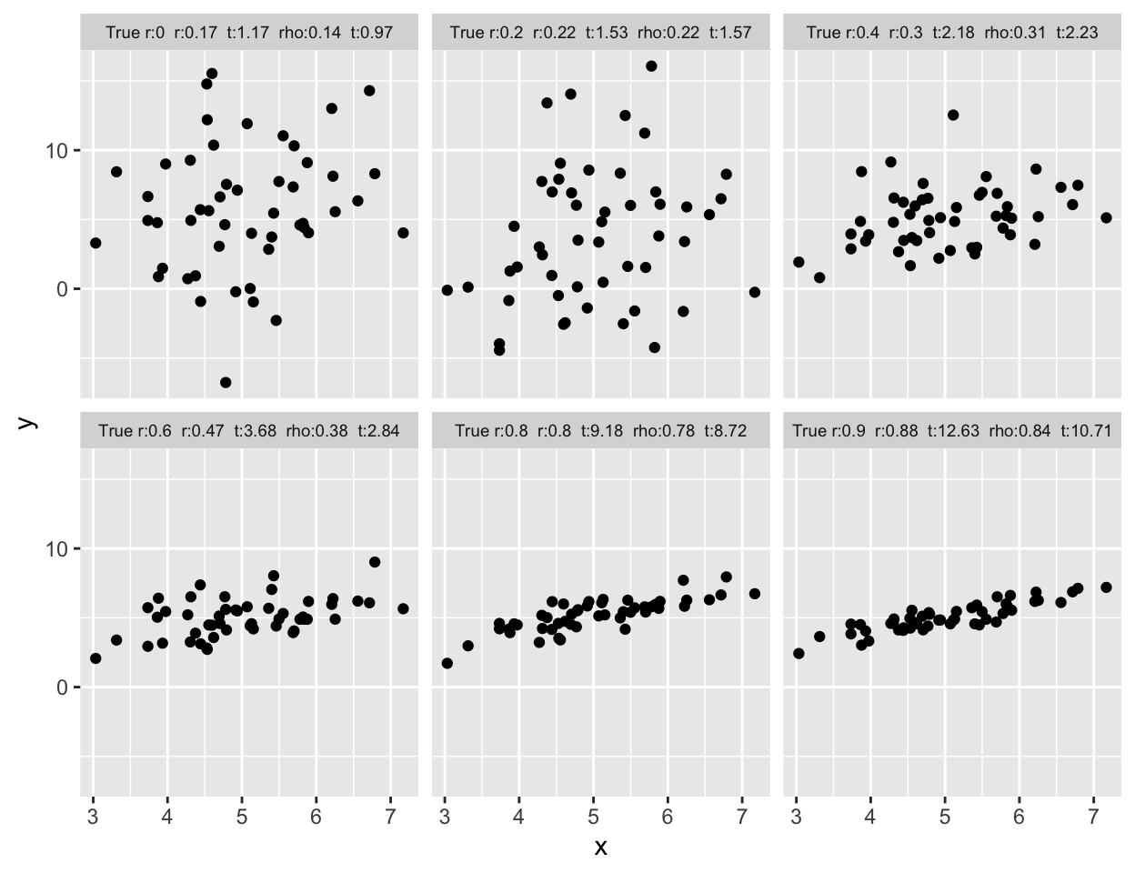
[1] 0.6951673[1] 0.6988119[1] 0.7014825[1] 0.701783[1] 0.6974104[1] 0.703308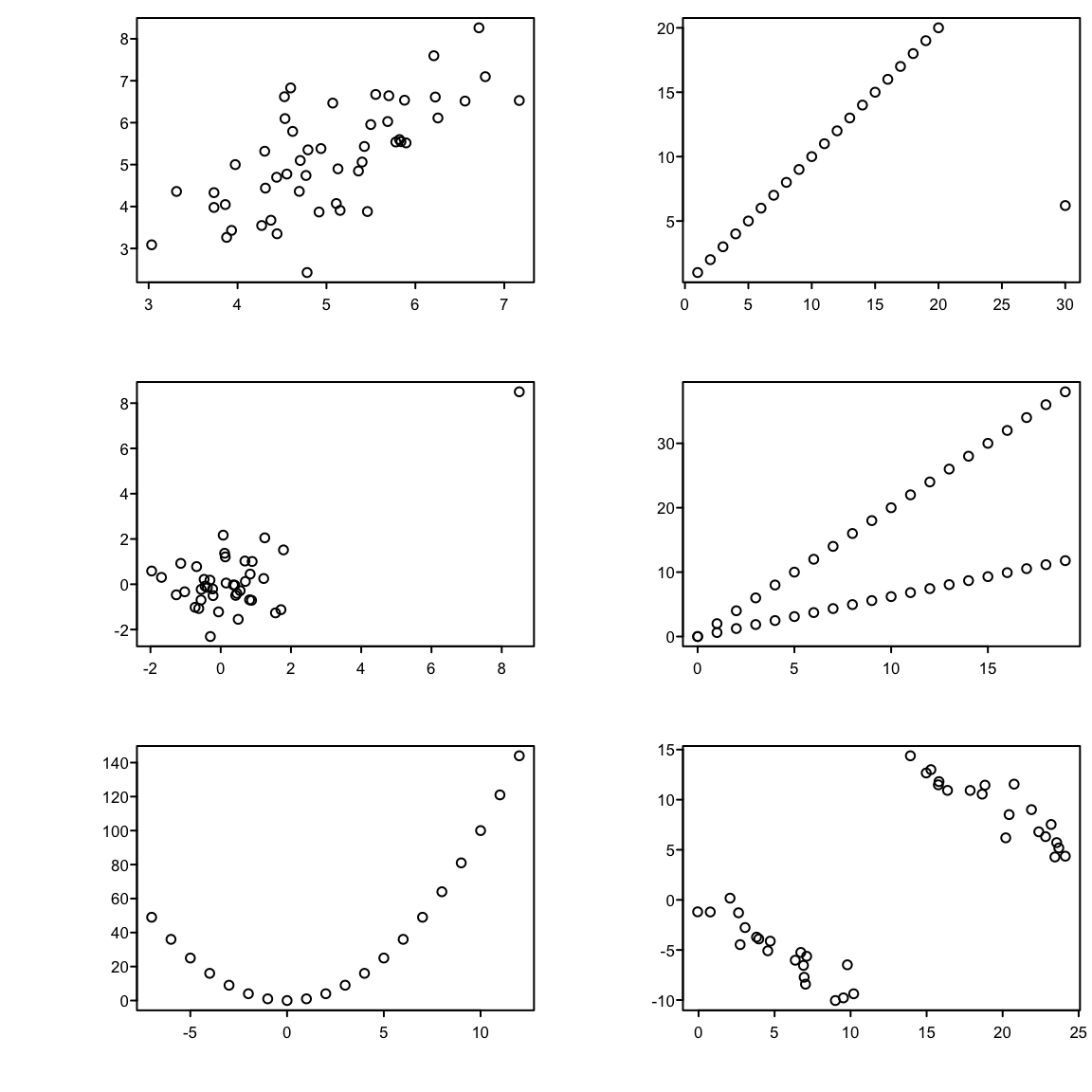
| \(r\) | \(\rho\) | |
|---|---|---|
| all data | 0.90 | 0.73 |
| avg pH \(\leq 4\) | 0.51 | 0.58 |
| avg pH \(> 4\) | 0.74 | 0.65 |
See Chapter 16 for simple approaches to assessing agreement and analyzing observer variability studies.
But there is controversy about what should be on the \(x\)-axis of the plot. Krouwer Krouwer (2008) concluded that:
require(Hmisc)
getHdata(esopH)
esopH$diff <- with(esopH, orophar - conv)
ggplot(esopH, aes(x=(conv + orophar)/2, y=diff)) +
stat_binhex(aes(fill=Hmisc::cut2(..count.., g=20)),
bins=80) +
stat_smooth() +
geom_hline(yintercept = mean(esopH$diff, na.rm=TRUE) +
c(-1.96, 0, 1.96) * sd(esopH$diff, na.rm=TRUE),
linetype=c(2,1,2), color='brown') +
xlab('Average of Conventional and Oropharyngeal pH') +
ylab('Oropharyngeal Minus Conventional pH') +
guides(fill=guide_legend(title='Frequency'))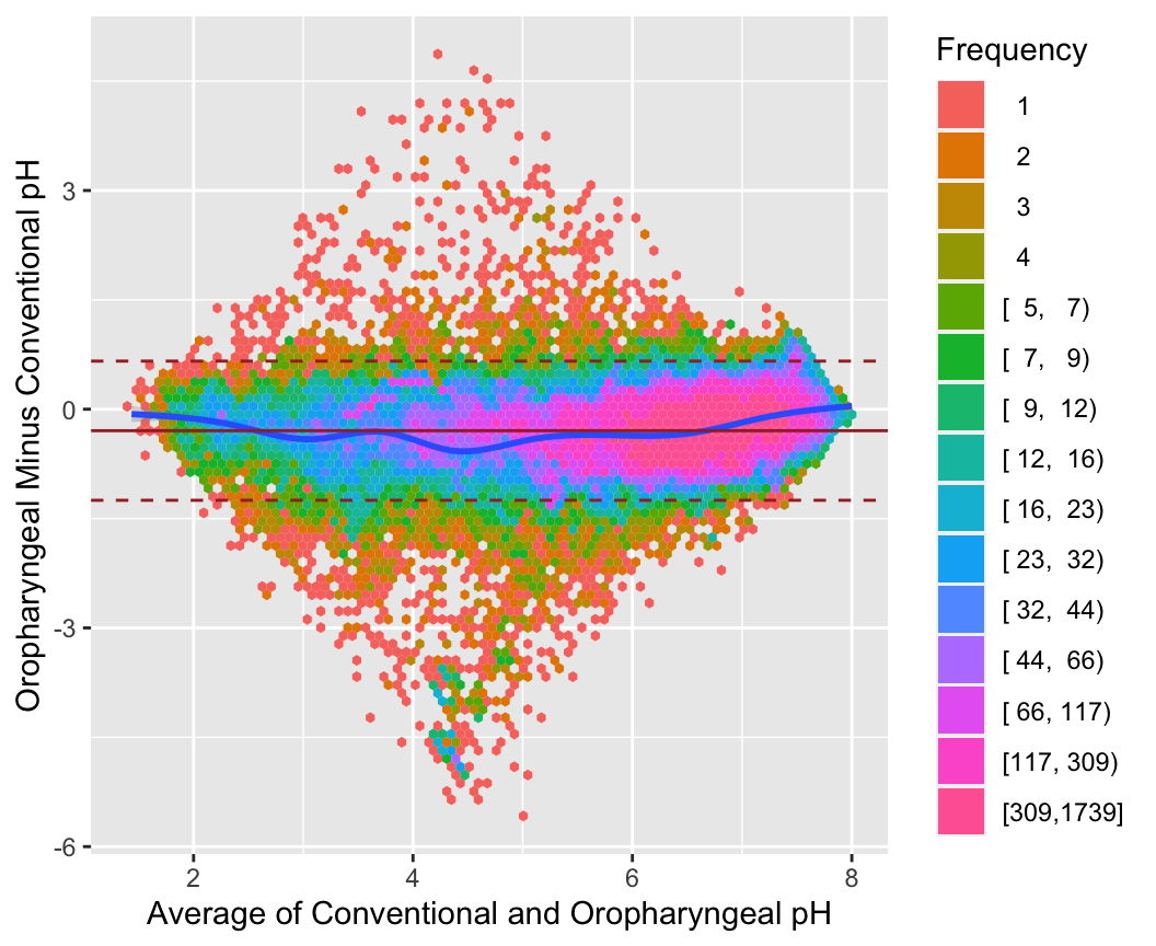
getHdata(esopH2)
ggplot(esopH2, aes(x=time, y=diffpH)) +
geom_point(pch='.') + stat_smooth() +
geom_hline(yintercept = 0, col='gray60') +
scale_x_continuous(breaks=seq(16, 38, by=4),
labels=c("4 PM", "8 PM", "12 AM",
"4 AM", "8AM", "12 PM"),
limits=c(14, 14+24)) +
ylab('Average of Oropharyngeal Minus Conventional pH') +
xlab('Time of Day')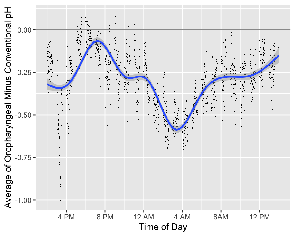
See also stats.stackexchange.com/questions/415131.
Another way to to compute needed sample size is to solve for \(n\) such that the probability that the observed correlation is in the right direction is high. Again using Fisher’s \(z\)-transformation \(z(r) = 0.5 \log{\frac{1 + r}{1 - r}}\), and letting \(r\) and \(\rho\) denote the sample and population correlation coefficients, respectively, \(z(r)\) is approximately normally distributed with mean \(z(\rho)\) and standard deviation \(\frac{1}{\sqrt{n-3}}\). The probability that \(r > 0\) is the same as \(\Pr(z(r) > 0)\), which equals \(\Pr(z(r) - z(\rho) > -z(\rho))\) = \(\Pr(\sqrt{n-3} z(r) - \sqrt{n-3} z(\rho) > -\sqrt{n-3} z(\rho))\) = \(\Phi(\sqrt{n-3}z(\rho))\), where \(\Phi\) is the \(n(0,1)\) cumulative distribution function. If we desired a probability of 0.95 of \(r\) having the right sign, we set the right hand side to 0.95 and solve for \(n\):
\[n = (\frac{\Phi^{-1}(0.95)}{z(\rho)})^{2} + 3\]
When the true correlation \(\rho\) is close to 0.0 it makes sense that the sample size required to be confidence that \(r\) is in the right direction is very large, and the direction will be very easy to determine if \(\rho\) is far from zero. So we are most interested in \(n\) when \(\rho \in [0.1, 0.5]\). The approximate sample sizes required for various \(\rho\) are shown in the graph below.
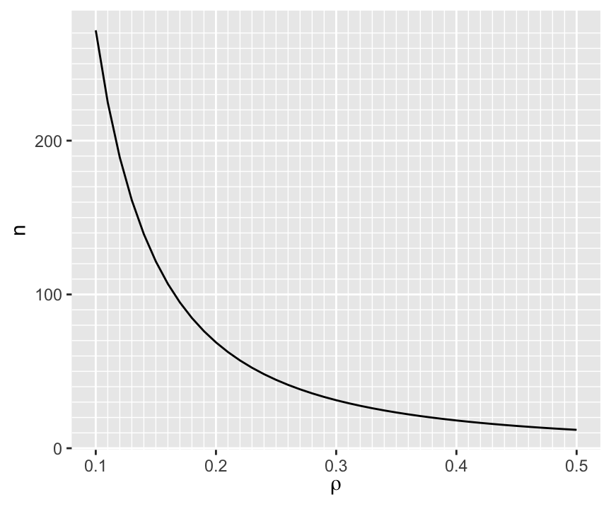
To have at least a 0.95 chance of being in the right direction when the true correlation is 0.1 (or -0.1) requires \(n > 250\).
For a given \(n\) we can compute the probability of being in the right direction for a few values of \(\rho\) as shown below.
d <- expand.grid(n=10:400, rho=c(0.01, 0.05, 0.1, 0.2, 0.3, 0.4, 0.5))
d <- transform(d, p=pnorm(sqrt(n - 3) * z(rho)))
ggplot(d, aes(x=n, y=p, color=factor(rho))) + geom_line() +
scale_x_continuous(minor_breaks=seq(10, 390, by=10)) +
scale_y_continuous(minor_breaks=seq(0.5, 1, by=0.01)) +
ylab('Pr(correct sign on r)') +
guides(color=guide_legend(title=expression(rho)))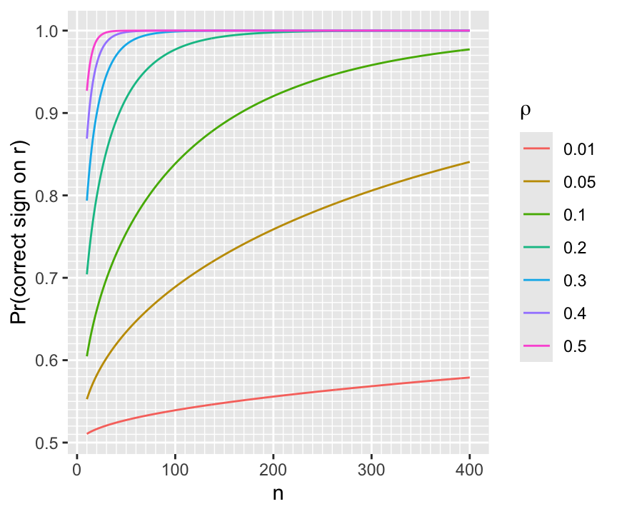
require(Hmisc)
require(mvtnorm)
# Get a population correlation matrix by getting sample correlations
# on a random normal sample with N=20 and all true correlations=0
# then pretend these sample correlations were real population values
set.seed(3)
x <- rmvnorm(20, sigma=diag(10))
R <- rcorr(x)$r
# True correlations we will simulate from:
round(R, 2) [,1] [,2] [,3] [,4] [,5] [,6] [,7] [,8] [,9] [,10]
[1,] 1.00 0.01 0.47 -0.09 -0.31 -0.07 0.14 0.05 0.02 -0.49
[2,] 0.01 1.00 0.48 0.27 0.27 0.14 0.40 -0.17 -0.59 0.60
[3,] 0.47 0.48 1.00 -0.11 0.26 -0.31 0.45 -0.12 -0.50 -0.06
[4,] -0.09 0.27 -0.11 1.00 0.42 0.42 -0.07 -0.35 0.16 0.35
[5,] -0.31 0.27 0.26 0.42 1.00 -0.04 0.03 -0.40 -0.25 0.34
[6,] -0.07 0.14 -0.31 0.42 -0.04 1.00 0.19 -0.36 0.08 0.40
[7,] 0.14 0.40 0.45 -0.07 0.03 0.19 1.00 -0.37 -0.65 -0.07
[8,] 0.05 -0.17 -0.12 -0.35 -0.40 -0.36 -0.37 1.00 0.17 -0.24
[9,] 0.02 -0.59 -0.50 0.16 -0.25 0.08 -0.65 0.17 1.00 -0.18
[10,] -0.49 0.60 -0.06 0.35 0.34 0.40 -0.07 -0.24 -0.18 1.00
-0.01 0 0.01
14 76 10 [,1] [,2] [,3] [,4] [,5] [,6] [,7] [,8] [,9] [,10]
[1,] 1.00 -0.01 0.50 0.11 0.00 -0.16 0.07 -0.04 -0.04 -0.43
[2,] -0.01 1.00 0.50 0.19 0.43 0.13 0.60 -0.26 -0.76 0.69
[3,] 0.50 0.50 1.00 -0.15 0.45 -0.41 0.52 -0.18 -0.58 -0.01
[4,] 0.11 0.19 -0.15 1.00 0.45 0.30 -0.13 -0.35 0.09 0.14
[5,] 0.00 0.43 0.45 0.45 1.00 -0.12 0.27 -0.53 -0.42 0.20
[6,] -0.16 0.13 -0.41 0.30 -0.12 1.00 0.06 -0.27 0.00 0.51
[7,] 0.07 0.60 0.52 -0.13 0.27 0.06 1.00 -0.57 -0.81 0.19
[8,] -0.04 -0.26 -0.18 -0.35 -0.53 -0.27 -0.57 1.00 0.37 -0.13
[9,] -0.04 -0.76 -0.58 0.09 -0.42 0.00 -0.81 0.37 1.00 -0.41
[10,] -0.43 0.69 -0.01 0.14 0.20 0.51 0.19 -0.13 -0.41 1.00r <- (0 : 3) / 4
n <- 50
zcrit <- qnorm(0.975)
z <- 0.5 * log( (1 + r) / (1 - r))
lo <- z - zcrit/sqrt(n-3)
hi <- z + zcrit/sqrt(n-3)
rlo <- (exp(2*lo)-1)/(exp(2*lo)+1)
rhi <- (exp(2*hi)-1)/(exp(2*hi)+1)
w <- rbind(r=r, 'Margin of Error'=pmax(rhi - r, r - rlo))
prmatrix(round(w, 2), collab=rep('', 4))
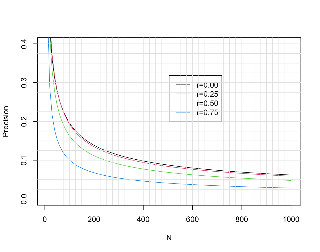
r 0.00 0.25 0.50 0.75
Margin of Error 0.28 0.28 0.24 0.15[1] 0.6854261[1] 38[1] 0.1149512
-0.3 -0.2 -0.1 0 0.1 0.2
2 6 7 7 17 6 # Repeat the "finding max r" procedure for 1000 bootstrap samples
# Sample from x 1000 times with replacement, each time computing
# a new correlation matrix
samepair <- dropsum <- 0
for(i in 1 : 1000) {
b <- sample(1 : 50, replace=TRUE)
xb <- x[b, ] # sample with replacement from rows
r <- rcorr(xb)$r
ru <- up(r)
wmax <- which.max(ru)
if(wmax == 38) samepair <- samepair + 1
# Compute correlation for the bootstrap best pair in the original sample
origr <- rorigu[wmax]
# Compute drop-off in best r
dropoff <- ru[wmax] - origr
dropsum <- dropsum + dropoff
}
cat('Number of bootstaps selecting the original most correlated pair:',
samepair, 'out of 1000', '\n')Number of bootstaps selecting the original most correlated pair: 642 out of 1000 Mean dropoff for max r: 0.071 # For each observed correlation compute its rank among 45 distinct pairs
orig.ranks <- rank(up(rorig))
# Sample from x 1000 times with replacement, each time computing
# a new correlation matrix
Rm <- matrix(NA, nrow=1000, ncol=45)
for(i in 1 : 1000) {
b <- sample(1 : 50, replace=TRUE)
xb <- x[b, ]
r <- rcorr(xb)$r
Rm[i, ] <- rank(up(r))
}
# Over bootstrap correlations compute quantiles of ranks
low <- apply(Rm, 2, quantile, probs=0.025)
high <- apply(Rm, 2, quantile, probs=0.975)
round(cbind('Original Rank'=orig.ranks, Lower=low, Upper=high)) Original Rank Lower Upper
[1,] 22 12 34
[2,] 40 32 45
[3,] 41 30 45
[4,] 28 15 37
[5,] 31 20 38
[6,] 15 8 28
[7,] 24 11 34
[8,] 37 32 43
[9,] 38 32 43
[10,] 39 31 44
[11,] 14 8 27
[12,] 29 15 37
[13,] 9 3 15
[14,] 35 22 43
[15,] 18 10 26
[16,] 26 16 34
[17,] 44 38 45
[18,] 43 34 45
[19,] 16 9 27
[20,] 34 25 38
[21,] 25 14 34
[22,] 19 11 32
[23,] 12 7 21
[24,] 13 7 27
[25,] 10 4 20
[26,] 5 3 10
[27,] 11 5 22
[28,] 4 3 8
[29,] 20 10 33
[30,] 2 1 4
[31,] 3 2 11
[32,] 27 16 36
[33,] 7 4 13
[34,] 23 13 32
[35,] 1 1 2
[36,] 36 28 43
[37,] 6 3 15
[38,] 45 40 45
[39,] 21 12 31
[40,] 30 17 37
[41,] 33 21 39
[42,] 42 34 44
[43,] 32 20 38
[44,] 17 11 28
[45,] 8 3 16ranks
34 35 36 37 38 39 40 41 42 43 44 45
2 1 6 8 10 18 25 38 58 88 152 594 2.5% 97.5%
38 45 [1] 0.26 -0.16 0.05 0.29 -0.03 0.04 0.28 0.05 0.28 0.57
-0.5 -0.4 -0.3 -0.2 -0.1 0 0.1 0.2 0.3 0.4 0.5
1 6 43 97 234 250 210 120 25 3 1 [1] 10[1] 0.5698995# Simulate 1000 repeats of sample with new y but keeping x the same
# See how original highest correlating variable ranks among 1000
# correlations in new samples
ranks <- numeric(1000)
for(i in 1 : 1000) {
ys <- Ey + rnorm(n) * 20
rs <- cor(x, ys)
ranks[i] <- rank(rs)[wmax]
}
table(round(ranks, -1)) # round to nearest 10
350 400 580 600 610 620 630 660 670 680 690 700 710 720 730 740
1 1 1 1 1 2 1 1 4 2 2 2 1 2 1 1
760 770 780 790 800 810 820 830 840 850 860 870 880 890 900 910
1 1 2 4 6 2 6 11 3 6 6 9 13 8 15 15
920 930 940 950 960 970 980 990 1000
15 34 39 41 50 66 126 203 294 2.5% 97.5%
770.85 1000.00 [1] 139RMS 2.4.7 ABD 17.8 🅓
| \(X\): | 1 | 2 | 3 | 5 | 8 |
|---|---|---|---|---|---|
| \(Y\): | 2.1 | 3.8 | 5.7 | 11.1 | 17.2 |
\[\begin{array}{ccc} \hat{E}(Y | X=2) &=& \frac{2.1+3.8+5.7}{3} \\ \hat{E}(Y | X=\frac{2+3+5}{3}) &=& \frac{3.8+5.7+11.1}{3} \end{array}\]
require(Hmisc)
require(data.table)
getHdata(abm) # Loads data frame ABM (note case)
# Convert to a data table and add derived variables
setDT(ABM)
ABM[, glratio := gl / bloodgl]
ABM[, tpolys := polys * whites / 100]
r <- ABM[, {
plsmo(tpolys, glratio, xlab='Total Polymorphs in CSF',
ylab='CSF/Blood Glucose Ratio',
xlim=quantile(tpolys, c(.05,.95), na.rm=TRUE),
ylim=quantile(glratio, c(.05,.95), na.rm=TRUE))
scat1d(tpolys); scat1d(glratio, side=4) } ]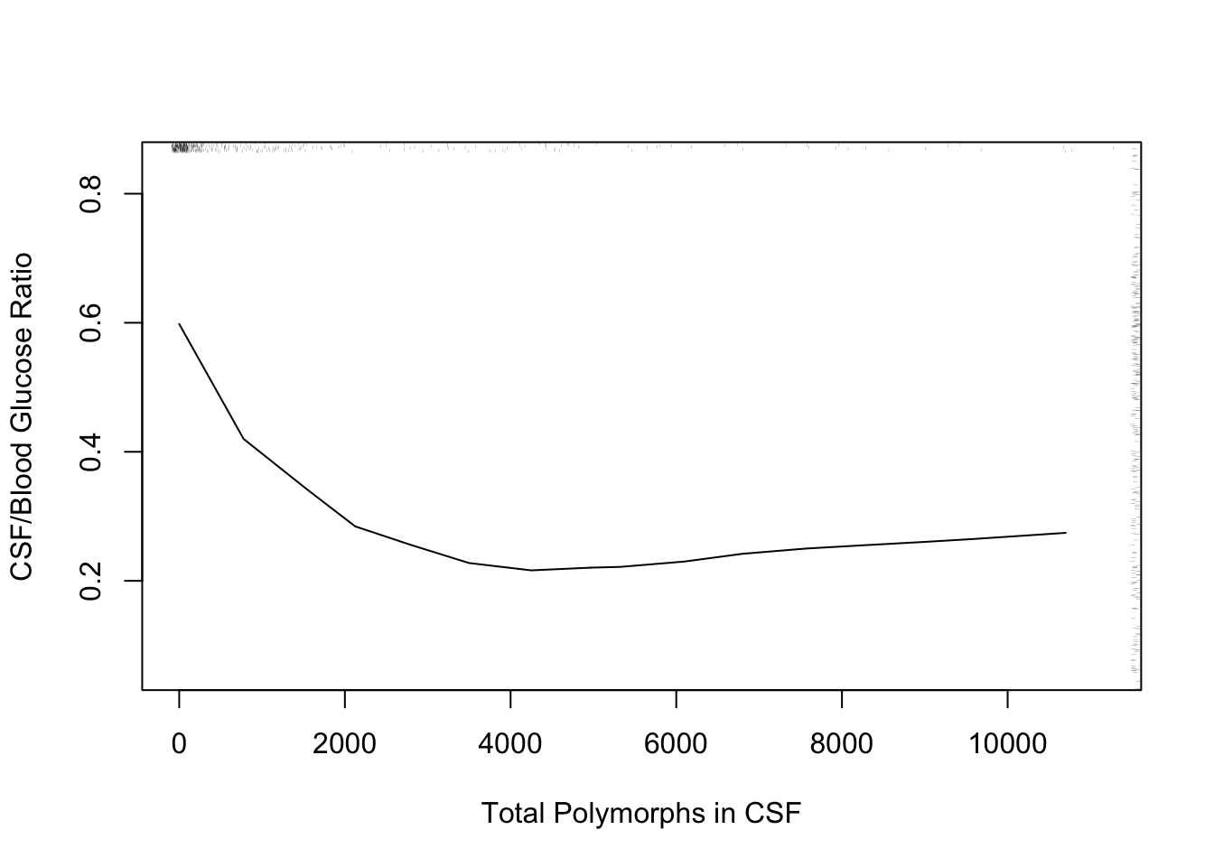
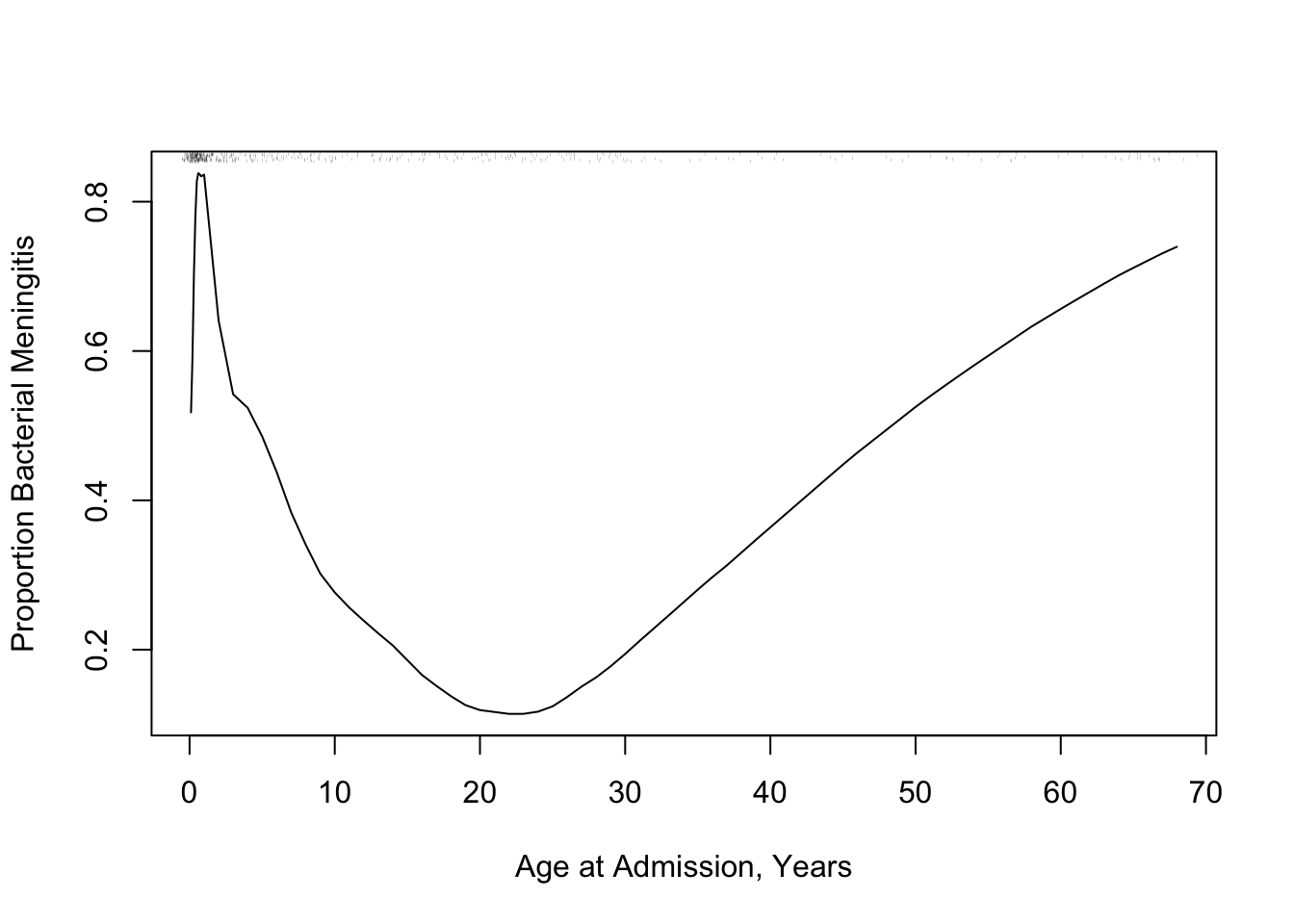
The following example using “super smoother” of Friedman (1984) in place of loess to estimate a complex relationship that has a sharp turn.
R function movStats in the Hmisc package|
Window Sample Sizes
|
||||
|---|---|---|---|---|
| N | Mean | Min | Max | xinc |
| 283 | 30.8 | 25 | 31 | 1 |
|
Window Sample Sizes
|
||||
|---|---|---|---|---|
| N | Mean | Min | Max | xinc |
| 420 | 30.9 | 25 | 31 | 2 |
|
Window Sample Sizes
|
||||
|---|---|---|---|---|
| N | Mean | Min | Max | xinc |
| 137 | 48.7 | 35 | 51 | 1 |
```{r setup, include=FALSE}
require(Hmisc)
require(qreport)
hookaddcap() # make knitr call a function at the end of each chunk
# to try to automatically add to list of figure
options(prType='html')
getRs('qbookfun.r')
knitr::set_alias(w = 'fig.width', h = 'fig.height',
cap = 'fig.cap', scap ='fig.scap')
ord <- markupSpecs$latex$ord # function to typeset ordinal integers
```
# Correlation and Nonparametric Regression
`r mrg(bmovie(12), ddisc(12))`
## Overview
| Outcome | Predictor | Normality? | Linearity? | Analysis Method |
|-----|-----|-----|-----|-----|
| Interval | Binary | Yes | | 2-sample $t$-test **or linear regression** |
| Ordinal | Binary | No | | Wilcoxon 2-sample test **or proportional odds model** |
| Categorical | Categorical | | | Pearson $\chi^2$ test |
| Interval | Interval | Yes | Yes | **Correlation or linear regression** |
| Ordinal | Ordinal | No | No | **Spearman's rank correlation** |
* Examine association between continuous/interval outcome ($y$) and continuous/interval predictor ($x$)
* Scatterplot of $y$ versus $x$
* Nonparametric smoother, including local linear regression, "super smoother", and overlapping moving windows for any statistic of interest
## Pearson's correlation coefficient
* $r = \frac{\Sigma(x_i - \bar{x})(y_i - \bar{y})}{\sqrt{\Sigma(x_i - \bar{x})^2\Sigma(y_i - \bar{y})^2}}$
* Range: $-1 \leq r \leq 1$
* Correlation coefficient is a unitless index of strength of association between two variables (+ = positive association, - = negative, 0 = no association)
* Measures the linear relationship between $X$ and $Y$
* Can test for significant association by testing whether the population correlation is zero
$$t = \frac{r\sqrt{n-2}}{\sqrt{1-r^{2}}}$$
which is identical to the $t$-test used to test whether the population
$r$ is zero; d.f.=$n-2$.
* Use probability calculator for $t$ distribution to get $P$-value (2-tailed if interested in association in either direction)
* 1-tailed test for a positive correlation between $X$ and $Y$ tests $H_{0}:$ when $X \uparrow$ does $Y \uparrow$ in the population?
* Confidence intervals for population $r$ calculated using Fisher's $Z$ transformation
$$Z = \frac{1}{2} \mathrm{log}_\mathrm{e} \left( \frac{1+r}{1-r} \right)$$
*
+ For large $n$, Z follows a Normal distribution with standard error $\frac{1}{\sqrt{n-3}}$
+ To calculate a confidence interval for $r$, first find the confidence interval for $Z$ then transform back to the $r$ scale
\begin{array}{ccc}
Z & = & \frac{1}{2} \mathrm{log}_\mathrm{e} \left( \frac{1+r}{1-r} \right) \\
2*Z & = & \mathrm{log}_\mathrm{e} \left( \frac{1+r}{1-r} \right) \\
\mathrm{exp}(2Z) & = & \left( \frac{1+r}{1-r} \right) \\
\mathrm{exp}(2Z) * (1-r) & = & 1 + r \\
\mathrm{exp}(2Z) - r * \mathrm{exp}(2Z) & = & 1 + r \\
\mathrm{exp}(2Z) - 1 & = & r * \mathrm{exp}(2Z) + r \\
\mathrm{exp}(2Z) - 1 & = & r \left(\mathrm{exp}(2Z) + 1\right) \\
\frac{\mathrm{exp}(2Z) - 1}{\mathrm{exp}(2Z) + 1} & = & r \\
\end{array}
* Example (Altman 89-90): Pearson's $r$ for a study investigating the association of basal metabolic rate with total energy expenditure was calculated to be $0.7283$ in a study of $13$ women. Derive a 0.95 confidence interval for $r$.
$$ Z = \frac{1}{2} \mathrm{log}_\mathrm{e} \left( \frac{1+0.7283}{1-0.7283} \right) = 0.9251 $$
The lower limit of a 0.95 CI for $Z$ is given by
$$ 0.9251 - 1.96 \times \frac{1}{\sqrt{13-3}} = 0.3053 $$
and the upper limit is
$$ 0.9251 + 1.96 \times \frac{1}{\sqrt{13-3}} = 1.545 $$
A 0.95 CI for the population correlation coefficient is given by transforming these limits from the $Z$ scale back to the $r$ scale
$$ \frac{\mathrm{exp}(2\times 0.3053) - 1}{\mathrm{exp}(2\times 0.3053) + 1} ~~~ \mathrm{to} ~~~ \frac{\mathrm{exp}(2\times 1.545) - 1}{\mathrm{exp}(2\times 1.545) + 1} $$
Which gives a 0.95 CI from 0.30 to 0.91 for the population correlation
```{r calcr}
n <- 13
r <- 0.7283
z.transform <- 0.5 * log((1 + r) / (1 - r))
clz <- z.transform + c(-1, 1) * qnorm(0.975) / sqrt(n - 3)
clr <- (exp(2 * clz) - 1) / (exp(2 * clz) + 1)
round(c(z.transform, clz, clr), 4)
```
## Spearman's Rank Correlation
* Pearson's $r$ assumes linear relationship between $X$ and $Y$
* Spearman's $\rho$ (sometimes labeled $r_{s}$) assumes monotonic relationship between $X$ and $Y$
+ when $X \uparrow$ $Y$ always $\uparrow$ or stays flat, or $Y$ always $\downarrow$ or stays flat
+ does not assume linearity
* $\rho = r$ once replace column of $X$s by their ranks and column of $Y$s by ranks
* To test $H_{0}:\rho=0$ without assuming linearity or normality, being damaged by outliers, or sacrificing much power (even if data are normal), use a $t$ statistic:
$$t = \frac{\rho\sqrt{n-2}}{\sqrt{1-\rho^{2}}}$$
which is identical to the $t$-test used to test whether the population
$r$ is zero; d.f.=$n-2$.
* Use probability calculator for $t$ distribution to get $P$-value (2-tailed if interested in association in either direction)
* 1-tailed test for a positive correlation between $X$ and $Y$ tests $H_{0}:$ when $X \uparrow$ does $Y \uparrow$ in the population?
## Correlation Examples
* Correlation difficult to judge by eye
* Example plots on following pages
```{r corrplota,w=6.5,h=5,cap='Samples of size $n=50$ for X and Y are drawn from bivariate normal populations with true correlations ranging from 0.0 to 0.9. Pearson and Spearman sample correlations are shown for samples of size 50. Besides the population correlation coefficient, each panel is labeled with the estimated Pearson $r$, its $t$ statistic, the estimated Spearman $\\rho$, and its $t$ statistic',scap='Example correlation coefficients'}
#| label: fig-corr-corrplota
# Generate 50 data points with Population correlations of 0, .2, .4, .6,
# .8, and .9 and plot results
require(ggplot2)
n <- 50
set.seed(123)
x <- rnorm(n, 5, 1)
d <- expand.grid(x=x, R=c(0, .2, .4, .6, .8, .9))
d <- transform(d, y = x + rnorm(nrow(d), 0,
ifelse(R == 0, 5, sqrt(R ^ -2 - 1))))
sfun <- function(i) {
x <- d$x[i]; y <- d$y[i]; R <- d$R[i][1]
r <- cor(x, y)
tr <- r * sqrt(n - 2) / sqrt(1 - r^2)
rho <- cor(rank(x), rank(y))
trho <- rho * sqrt(n - 2) / sqrt(1 - rho^2)
label <- paste('True r:', R[1], ' r:', round(r,2), ' t:', round(tr,2),
' rho:', round(rho,2), ' t:', round(trho,2), sep='')
names(label) <- R
label
}
stats <- tapply(1 : nrow(d), d$R, sfun)
d$stats <- factor(stats[as.character(d$R)], unique(stats))
ggplot(d, aes(x=x, y=y)) + geom_point() + facet_wrap(~ stats) +
theme(strip.text.x = element_text(size=7))
```
```{r corrplotb,w=6,h=6,cap='Different observed datasets that have the same correlation. All six plots have a sample Pearson correlation of $0.7$.',scap='Multiple datasets having same Pearson $r$'}
#| label: fig-corr-corrplotb
# Different scenarios that can lead to a correlation of 0.7
spar(mfrow=c(3,2))
set.seed(123)
rho <- 0.7; n <- 50
var.eps <- rho^-2 - 1
x <- rnorm(n, 5, 1)
y <- x + rnorm(n, 0, sqrt(var.eps))
cor(x,y)
plot(x,y,xlab='',ylab='')

x <- c(1:20,30)
y <- c(1:20,6.2)
cor(x,y)
plot(x,y,xlab='',ylab='')

set.seed(123)
x <- rnorm(40)
y <- rnorm(40)
x[21] <- y[21] <- 8.5
cor(x,y)
plot(x,y,xlab='',ylab='')

x <- rep(0:19,2)
y <- c(rep(.62,20),rep(2,20)) * x
cor(x,y)
plot(x,y,xlab='',ylab='')

x <- -7:12
y <- x^2
cor(x,y)
plot(x,y,xlab='',ylab='')

set.seed(123)
tmp <- 1:20 / 2
x <- c(rnorm(20, tmp, 1), tmp + rnorm(20,14.5,1))
y <- c(rnorm(20, -tmp, 1), -tmp + rnorm(20,14.5,1))
cor(x,y)
plot(x,y,xlab='',ylab='')
```
## Correlation and Agreement
* Compare two methods of measuring the same underlying value
+ Lung function measured using a spirometer (expensive, accurate) or peak flow meter (cheap, less accurate)
+ Two devices (oropharyngeal and conventional) used to measure acidity (pH) in the esophagus as a marker of reflux
* Typical (incorrect) approach begins with scatterplot of one method vs. the other with a 1:1 line indicating perfect agreement
* See @fig-descript-ph
* Incorrect approach would report a high correlation ($r = 0.90$) and conclude good agreement
* Problems with the correlation approach
1. $r$ measures the degree of linear association between two variables, not the agreement. If, for example, the Sandhill consistently gave pH values that were 0.5 unit higher than the Restech, we could still have high correlation, but poor agreement between the two devices. We can have high correlation if the two devices lie closely to any line, not just a 1:1 line that indicates perfect agreement.
1. A change in scale does not affect correlation, but does influence agreement. For example, if the Sandhill always registered 2 times larger than the Restech, we would have perfect correlation but the agreement would get progressively worse for larger values of pH.
1. Correlation depends on the range of the data so that larger ranges lead to larger correlations. This can lead to vary strange interpretations
| | $r$ | $\rho$ |
|-----|-----|-----|
| all data | 0.90 | 0.73 |
| avg pH $\leq 4$ | 0.51 | 0.58 |
| avg pH $> 4$ | 0.74 | 0.65 |
: Pearson ($r$) and Spearman ($\rho$) correlations for Restech and Sandhill pH data. The correlation calculated using all of the data is larger than the correlation calculated using a restricted range of the data. However, it would be difficult to claim that the overall agreement is better than both the agreement when pH is less than 4 and when pH is greater than 4.
1. Tests of significance (testing if $r=0$) are irrelevant to the question at hand, but often reported to demonstrate a significant association. The two devices are measuring the same quantity, so it would be shocking if we did not observe a highly significant $p$-value. A $p < .0001$ is not impressive. A regression analysis with a highly significant slope would be similarly unimpressive.
1. Data can have high correlation, but poor agreement. There are many examples in the literature, but even in our analysis with $r = 0.90$, the correlation is high, but we will show that the agreement is not as good as the high correlation implies.
See @sec-obsvar for simple approaches to assessing agreement
and analyzing observer variability studies.
### Bland-Altman Plots
`r mrg(ems("36.4"))`
* See Bland and Altman (1986, Lancet)
* Earlier: Tukey mean-difference plot
* Create plots of the difference in measurements on the y-axis versus the average value of the two devices on the x-axis
* If the two devices agree, the difference should be about zero
* The average of the two devices is our best estimate of the true, unknown (pH) value that is we are trying to measure
* Measurements will often vary in a systematic way over the range of measurement. By plotting the difference versus the average, we can visually determine if the difference changes over our estimate of the truth.
* Solid line indicated the mean, dashed lines are approximate 0.95 confidence intervals (assuming Normality)
**But** there is controversy about what should be on the $x$-axis
of the plot. Krouwer @kro08why concluded that:
* When the two measures have nearly equal variability, i.e., when comparing two "field measurements", the Bland-Altman approach is preferred
* When one measurement is a "reference standard" having much less variation than the field measurement, the reference standard and not the average of the two measurements should be on the $x$-axis
```{r baplot,w=5.5,h=4.5,cap='Bland-Altman plot for the oroesophageal and conventional pH measurements, using hexagonal binning because of the large sample size. The difference in pH mesaurements (oro.\\ -conventional) is presented on the $y$-axis and the average of the two devices on the $x$-axis. We see poor agreement around pH values of 4-5',scap='Bland-Altman plot for 2 pH measurements'}
#| label: fig-corr-baplot
require(Hmisc)
getHdata(esopH)
esopH$diff <- with(esopH, orophar - conv)
ggplot(esopH, aes(x=(conv + orophar)/2, y=diff)) +
  stat_binhex(aes(fill=Hmisc::cut2(..count.., g=20)),
              bins=80) +
  stat_smooth() +
  geom_hline(yintercept = mean(esopH$diff, na.rm=TRUE) +
   c(-1.96, 0, 1.96) * sd(esopH$diff, na.rm=TRUE),
   linetype=c(2,1,2), color='brown') +
  xlab('Average of Conventional and Oropharyngeal pH') +
  ylab('Oropharyngeal Minus Conventional pH') +
  guides(fill=guide_legend(title='Frequency'))
```
* We will also consider differences in the two measurements over the time of day
* The added smooth curve is called a locally weighted scatterplot smooth (loess)
```{r phtimediff,w=5,h=4,cap='Difference in pH measurements (oro. - conventional) by time of day along with a loess smoother and pointwise 0.95 confidence bands. Is the difference modified by a subject being in a supine position rather than being upright?',scap='Difference in pH by time of day'}
#| label: fig-corr-phtimediff
getHdata(esopH2)
ggplot(esopH2, aes(x=time, y=diffpH)) +
       geom_point(pch='.') + stat_smooth() +
       geom_hline(yintercept = 0, col='gray60') +
       scale_x_continuous(breaks=seq(16, 38, by=4),
                          labels=c("4 PM", "8 PM", "12 AM",
                            "4 AM", "8AM", "12 PM"),
                          limits=c(14, 14+24)) +
       ylab('Average of Oropharyngeal Minus Conventional pH') +
       xlab('Time of Day')
```
### Sample Size for $r$ {#sec-corr-n}
* Without knowledge of population variances, etc., $r$ can be useful for planning studies
* Choose $n$ so that margin for error (half-width of C.L.) for $r$ is acceptable
* Precision of $r$ in estimating $\rho$ is generally worst when $\rho=0$
* This margin for error as well as that for three other choices of the unknown true $\rho$ are shown in @fig-corr-moe.
```{r moe,w=7,h=5.5,cap='Margin for error (length of longer side of asymmetric 0.95 confidence interval) for $r$ in estimating $\\rho$, when $\\rho=0, 0.25, 0.5, 0.75$. Calculations are based on Fisher $z$ transformation of $r$.',scap='Margin of error for estimating correlation coefficient'}
#| label: fig-corr-moe
require(Hmisc)
plotCorrPrecision(rho=c(0, .25, .5, .75),
                  n=seq(10, 1000, length=100),
                  ylim=c(0, .4), col=1:4, opts=list(keys='lines'))
abline(h=seq(0, .4, by=0.025),
       v=seq(25, 975, by=25), col=gray(.9))
```
See also [stats.stackexchange.com/questions/415131](https://stats.stackexchange.com/questions/415131).
Another way to to compute needed sample size is to solve for $n$ such that the probability that the observed correlation is in the right direction is high. Again using Fisher's $z$-transformation $z(r) = 0.5 \log{\frac{1 + r}{1 - r}}$, and letting $r$ and $\rho$ denote the sample and population correlation coefficients, respectively, $z(r)$ is approximately normally distributed with mean $z(\rho)$ and standard deviation $\frac{1}{\sqrt{n-3}}$. The probability that $r > 0$ is the same as $\Pr(z(r) > 0)$, which equals $\Pr(z(r) - z(\rho) > -z(\rho))$ = $\Pr(\sqrt{n-3} z(r) - \sqrt{n-3} z(\rho) > -\sqrt{n-3} z(\rho))$ = $\Phi(\sqrt{n-3}z(\rho))$, where $\Phi$ is the $n(0,1)$ cumulative distribution function. If we desired a probability of 0.95 of $r$ having the right sign, we set the right hand side to 0.95 and solve for $n$:
$$n = (\frac{\Phi^{-1}(0.95)}{z(\rho)})^{2} + 3$$
When the true correlation $\rho$ is close to 0.0 it makes sense that the sample size required to be confidence that $r$ is in the right direction is very large, and the direction will be very easy to determine if $\rho$ is far from zero. So we are most interested in $n$ when $\rho \in [0.1, 0.5]$. The approximate sample sizes required for various $\rho$ are shown in the graph below.
```{r w=4.5,h=3.75}
#| label: fig-corr-direction
#| fig-cap: "Sample size required to ensure a high probability of the sample correlation coefficient being in the right direction"
z   <- function(x) 0.5 * log((1 + x) / (1 - x))
rho <- seq(0.1, 0.5, by=0.01)
n   <- 3 + (qnorm(0.95) / z(rho)) ^ 2
ggplot(mapping=aes(x=rho, y=n)) + geom_line() +
  scale_x_continuous(minor_breaks=seq(0.1, 0.5, by=0.01)) +
  scale_y_continuous(minor_breaks=seq(10, 270, by=10)) +
  xlab(expression(rho))
```
To have at least a 0.95 chance of being in the right direction when the true correlation is 0.1 (or -0.1) requires $n > 250$.
For a given $n$ we can compute the probability of being in the right direction for a few values of $\rho$ as shown below.
```{r w=4.5,h=3.75}
#| label: fig-corr-ndirection
#| fig-cap: "Probability of having the correct sign on $r$ as a function of $n$ and true correlation $\\rho$"
d <- expand.grid(n=10:400, rho=c(0.01, 0.05, 0.1, 0.2, 0.3, 0.4, 0.5))
d <- transform(d, p=pnorm(sqrt(n - 3) * z(rho)))
ggplot(d, aes(x=n, y=p, color=factor(rho))) + geom_line() +
  scale_x_continuous(minor_breaks=seq(10, 390, by=10)) +
  scale_y_continuous(minor_breaks=seq(0.5, 1, by=0.01)) +
  ylab('Pr(correct sign on r)') +
  guides(color=guide_legend(title=expression(rho)))
```
### Comparing Two $r$'s
* Rarely appropriate
* Two $r$'s can be the same even though slopes may differ
* Usually better to compare effects on a real scale (slopes)
## Avoiding Overinterpretation
* Often researchers
+ compute many correlations then
+ make a big deal out of the largest observed correlation
* This is _double dipping_: using the same dataset to tell you which features to test, then testing those features
* This is a ranking and selection problem, and the data seldom contain enough information to be reliable in the choices
### Simulate Data
* For our analysis experiments, simulate a sample of size 50 from a 10-variate normal distribution with a known correlation matrix
* To specify this correlation matrix take the easy way out: compute an observed correlation matrix from a small sample where all correlations in the population are zero
* The usual sample noise will generate some large observed correlations
```{r simrdat}
require(Hmisc)
require(mvtnorm)
# Get a population correlation matrix by getting sample correlations
# on a random normal sample with N=20 and all true correlations=0
# then pretend these sample correlations were real population values
set.seed(3)
x <- rmvnorm(20, sigma=diag(10))
R <- rcorr(x)$r
# True correlations we will simulate from:
round(R, 2)
# Get a huge sample from a multivariate normal distribution to see
# that it mimics the real correlation matrix R
x <- rmvnorm(50000, sigma=R)
table(round(R - rcorr(x)$r, 2))
# Now sample from the population to get our dataset with N=50
x <- rmvnorm(50, sigma=R)
rorig <- rcorr(x)$r
round(rorig, 2)
```
### Margin of Error for a Single $r$
* First compute the margin of error in estimating a single $r$ from $n=50$
* This is the spacing between $r$ and it's lower 0.95 CL or the spacing between $r$ and its upper CL whichever is greatest
* CL based on Fisher's $z$-transformation described earlier
* Compute this for 4 hypothetical true $r$: 0 0.25 0.5 0.75
```{r rmoe}
r <- (0 : 3) / 4
n <- 50
zcrit <- qnorm(0.975)
z <- 0.5 * log( (1 + r) / (1 - r))
lo <- z - zcrit/sqrt(n-3)
hi <- z + zcrit/sqrt(n-3)
rlo <- (exp(2*lo)-1)/(exp(2*lo)+1)
rhi <- (exp(2*hi)-1)/(exp(2*hi)+1)
w <- rbind(r=r, 'Margin of Error'=pmax(rhi - r, r - rlo))
prmatrix(round(w, 2), collab=rep('', 4))
```
* If the true correlation is 0.5, the margin of error in estimating it is $\pm 0.24$ with $n=50$
### Bootstrapping the Correlation Selection Process
* Can use the bootstrap to document the difficulty of the task
* Steps:
1. form a matrix with $N$ rows and $p$ columns where $N$ is the number of observations and $p$ is the number of variables being correlated with each other
1. draw a sample of size $N$ from this matrix by sampling its rows
1. compute all the correlation coefficients as was done previously
1. re-run the same selection process as was done on the original dataset
1. repeat 1000 times
1. examine the distribution of the selections over the 1000 repeats
### Bootstrapping Bias in Largest Observed $r$
* Start with something simpler than ranking all the $r$s in the matrix: estimate the bias in the largest observed $r$
* Draw a sample with replacement from rows of the data matrix
* For each of these bootstrap samples find which pair of variables has the highest $r$
* Track this variable pair and compute $r$ in the original sample
* Compute the drop-off in $r$ from the bootstrap sample to the original sample
* This simulates the _process_ used to find the largest $r$
* Example: use data simulated above with 10 standard normal random variables \& known correlation matrix on 50 subjects
* Sample correlation matrix has $\frac{10 \times 9}{2} = 45$ distinct coefficients
```{r bootmax}
# Function to retrieve the upper triangle of a symmetric matrix
# ignoring the diagonal terms
up <- function(z) z[upper.tri(z)]
rorigu <- up(rorig)
max(rorigu)   # .685 = [2,10] element; 0.604 in population
which.max(rorigu)
# is the 38th element in the upper triangle

# Tabulate the difference between sample r estimates and true values
Ru <- up(R)
mean(abs(Ru - rorigu))
table(round(Ru - rorigu, 1))
# Repeat the "finding max r" procedure for 1000 bootstrap samples
# Sample from x 1000 times with replacement, each time computing
# a new correlation matrix
samepair <- dropsum <- 0
for(i in 1 : 1000) {
  b  <- sample(1 : 50, replace=TRUE)
  xb <- x[b, ]   # sample with replacement from rows
  r  <- rcorr(xb)$r
  ru <- up(r)
  wmax <- which.max(ru)
  if(wmax == 38) samepair <- samepair + 1
  # Compute correlation for the bootstrap best pair in the original sample
  origr <- rorigu[wmax]
  # Compute drop-off in best r
  dropoff <- ru[wmax] - origr
  dropsum <- dropsum + dropoff
}
cat('Number of bootstaps selecting the original most correlated pair:',
    samepair, 'out of 1000', '\n')
cat('Mean dropoff for max r:', round(dropsum / 1000, 3), '\n')
```
* For our dataset with $n=50$ we expect that the maximum observed $r$ out of 45 $r$s is biased high by 0.071
+ Could subtract 0.071 to debias the observed max $r$ although this will worsen its precision
### Bootstrapping Ranks of All $r$s
* Do a more comprehensive assessment that quantifies the difficulty of the task in ranking all the $r$s
* Quantity uncertainties in the ranks of the original correlation coefficients
* Apparent "winner" was the one receiving the highest ranking
$q$ among all $r$s
* What is the distribution of $q$ over the 1000 bootstrap samples?
* Can easily compute a 0.95 bootstrap nonparametric percentile confidence interval for the true unknown ranking of that feature combination and for ranking all the examined feature correlations
* Bootstrap the correlation matrix and re-rank the coefficients
* For each pair of variables compute the 0.95 confidence interval for the rank of its correlation from among the 45
```{r bootcorr}
# For each observed correlation compute its rank among 45 distinct pairs
orig.ranks <- rank(up(rorig))
# Sample from x 1000 times with replacement, each time computing
# a new correlation matrix
Rm <- matrix(NA, nrow=1000, ncol=45)
for(i in 1 : 1000) {
  b  <- sample(1 : 50, replace=TRUE)
  xb <- x[b, ]
  r  <- rcorr(xb)$r
  Rm[i, ] <- rank(up(r))
}
# Over bootstrap correlations compute quantiles of ranks
low  <- apply(Rm, 2, quantile, probs=0.025)
high <- apply(Rm, 2, quantile, probs=0.975)
round(cbind('Original Rank'=orig.ranks, Lower=low, Upper=high))
```
* Highest observed $r$ (rank 45) has 0.95 CI $[40,45]$
* Data are consistent with it being the `r ord(6)` highest
* Smallest observed value (rank 1; most impressive negative correlation) has CI $[1, 2]$ for rank; data consistent with that pair of variables being the best or `r ord(2)`
* The $r$ originally ranked `r ord(36)` has a 0.95 CI of $[28, 43]$ so the data are consistent with it being in the top 3
### Monte Carlo Simulation to Get A Rank Interval
* For comparison with the bootstrap, get the frequency distribution of ranks in repeated studies of the apparently highest $r$ in our $n=50$ study
* Repeated studies will also have $n=50$ and will be generated from the population correlation matrix
* Recall that original max $r$ was the `r ord(38)` element of the strung-out $r$ matrix from our sample
```{r mc}
ranks <- integer(1000)
for(i in 1 : 1000) {
  xs <- rmvnorm(50, sigma=R)
  rsim <- up(rcorr(xs)$r)
  ranks[i] <- rank(rsim)[38]
}
table(ranks)   # freqs. of ranks of 38th element in new samples
quantile(ranks, c(0.025, 0.975))
```
* This interval is a bit wider than the bootstrap interval
* **Note**: both the bootstrap and the Monte Carlo simulated interval would be **far wider** had the number of correlation coefficients estimated been much greater than the sample size
* Example: consider 1000 possible associations with a single $Y$
* This time the potential predictors $X$ will be independent in the population and they will be conditioned on (held constant over simulations at the original $X$ values)
* The true importance of the $X$s is $1, 2, \ldots, 10$ for the first 10 and all remaining are irrelevant in the population
```{r bigp}
set.seed(8)
n <- 50
p <- 1000
x <- matrix(rnorm(n * p), ncol=p)
Ey <- x[,1] + 2 * x[,2] + 3 * x[,3] + 4 * x[,4] + 5 * x[,5] + 6 * x[,6] +
      7 * x[,7] + 8 * x[,8] + 9 * x[,9] + 10 * x[,10]
y <- Ey + rnorm(n) * 20
ro <- cor(x, y)
# First 10 correlations and tabulate all others
round(ro[1:10], 2)
table(round(ro[-(1:10)], 1))
# Find which of the 1000 correlation against Y is largest
wmax <- which.max(ro)
wmax     # correct according to population
ro[wmax] # original rank=1000
# Simulate 1000 repeats of sample with new y but keeping x the same
# See how original highest correlating variable ranks among 1000
# correlations in new samples

ranks <- numeric(1000)
for(i in 1 : 1000) {
  ys <- Ey + rnorm(n) * 20
  rs <- cor(x, ys)
  ranks[i] <- rank(rs)[wmax]
}

table(round(ranks, -1))   # round to nearest 10
quantile(ranks, c(0.025, 0.975))
sum(ranks > 998)
```
* The apparent winning variable could fairly easily be the `r ord(771)` largest instead of the `r ord(1000)` ranked correlation
* The winning variable was in the top two in only 139 out of 1000 simulations
* See Chapter @sec-hdata for more ways to quantify limitations of high-dimensional data analysis, including the $p > N$ case
## Nonparametric Regression
`r mrg(bookref("RMS", "2.4.7"), abd("17.8"), disc("reg-nonpar"))`
* Linearity of relationships is often assumed; not a realistic assumption
* Nonparametric regression is an excellent descriptive tool that does not assume linearity; only assumes smoothness
* Estimates tendency of $Y$ (e.g., mean, median) as a function of a continuous $X$
* Estimates shape and steepness of the relationship
* Few assumptions
* Especially handy when there is a single $X$
* Plotted trend line may be the final result of the analysis
* Simplest smoother: moving average
* Example with unequally-spaced $X$
* Typical approach linking mean of $X$ in an interval with mean of $Y$ for that $X$-interval
| $X$: | 1 | 2 | 3 | 5 | 8 |
|-----|-----|-----|-----|-----|-----|
| $Y$: | 2.1 | 3.8 | 5.7 | 11.1 | 17.2 |
$$\begin{array}{ccc}
\hat{E}(Y | X=2) &=& \frac{2.1+3.8+5.7}{3} \\
\hat{E}(Y | X=\frac{2+3+5}{3}) &=& \frac{3.8+5.7+11.1}{3}
\end{array}$$
* overlap OK
* problem in estimating $E(Y)$ at outer $X$-values
* estimates very sensitive to bin width
* Moving linear regression superior to moving avg. (moving flat line)
* Cleveland's moving linear regression smoother _loess_ (locally weighted least squares) is the most popular smoother
* @fig-corr-phtimediff introduced us to _loess_
* Another example: differential diagnosis of acute bacterial meningitis
vs. viral meningitis
```{r glratio}
#| label: fig-corr-glratio
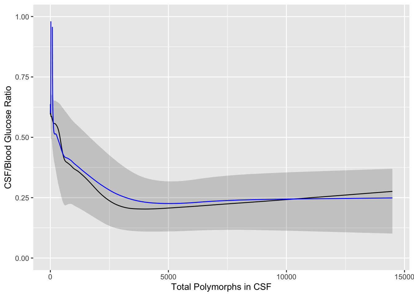
#| fig-cap: '_loess_ nonparametric smoother relating CSF:blood glucose ratio to total CSF polymorph count in patients with either bacterial or viral meningitis. Rug plot on axes plots indicate raw data values.'
#| fig-scap: '_loess_ nonparametric smoother for glucose ratio'
require(Hmisc)
require(data.table)
getHdata(abm)   # Loads data frame ABM (note case)
# Convert to a data table and add derived variables
setDT(ABM)
ABM[, glratio := gl / bloodgl]
ABM[, tpolys  := polys * whites / 100]
r <- ABM[, {
  plsmo(tpolys, glratio, xlab='Total Polymorphs in CSF',
       ylab='CSF/Blood Glucose Ratio',
       xlim=quantile(tpolys,  c(.05,.95), na.rm=TRUE),
       ylim=quantile(glratio, c(.05,.95), na.rm=TRUE))
 scat1d(tpolys); scat1d(glratio, side=4) } ]
```
The following example using "super smoother" of @fri84var in place of _loess_ to estimate a complex relationship that has a sharp turn.
```{r age-abm}
#| label: fig-corr-age-abm
#| fig-cap: '_Super smoother_ relating age to the probability of bacterial meningitis given a patient has bacterial or viral meningitis, with a rug plot showing the age distribution.'
#| fig-scap: "Example of super smoother"
r <- ABM[, {
  plsmo(age, abm, 'supsmu', bass=7,
        xlab='Age at Admission, Years',
        ylab='Proportion Bacterial Meningitis')
  scat1d(age) } ]
```
* In both examples there is strong non-linearity, even non-monotonicity
* But _loess_ and the super smoother are limited to estimating a mean or proportion
* Idea of moving average can be extended to all types of $Y$, even censored survival times
* Consider overlapping windows in which we compute moving _statistics_ in general
* See [here](http://hbiostat.org/rflow/analysis.html#descriptively-relating-one-variable-to-another) for details and several examples
* Brief idea:
+ create overlapping moving windows of $X$
+ for each window compute the statistic on $Y$
+ link it with the mean of $X$ for that window
+ advance $X$ by a small amount and repeat
* Smaller windows $\rightarrow$ noisier estimates of $Y$ but avoid bias
* Smooth the moving estimates using _loess_ or super smoother when finished
* To handle skewed $X$ it's best to form windows on the basis of sample size rather than on absolute $X$
* General `R` function `movStats` in the `Hmisc` package
* Default algorithm:
+ sort the data by $X$
+ get a target grid of $X$ values for which to estimate $Y$ separately
+ take 15 observations to the left of the target $X$ and 15 to the right as the window
+ for each new calculation move up $\frac{n}{200}$ observations (1 observation if $n < 200$) to form the new window
* Example using the glucose data but estimating 3 quartiles plus the mean
```{r results='asis'}
#| label: fig-corr-glratiom
#| fig-cap: 'Moving quartiles and mean (blue line) to relate CSF:blood glucose ratio to total CSF polymorph count in patients with either bacterial or viral meningitis. Black line is the moving median. The band depicts outer quartiles.'
#| fig-scap: 'Moving statistics for glucose ratio'
u <- movStats(glratio ~ tpolys, data=ABM, pr='margin')
ggplot(u, aes(x=tpolys, y=`Moving Median`)) + geom_line() +
    geom_ribbon(aes(ymin=`Moving Q1`, ymax=`Moving Q3`), alpha=0.2) +
  geom_line(aes(x=tpolys, y=`Moving Mean`, col=I('blue'))) +
    xlab('Total Polymorphs in CSF') +
    ylab('CSF/Blood Glucose Ratio') + ylim(0, 1)
```
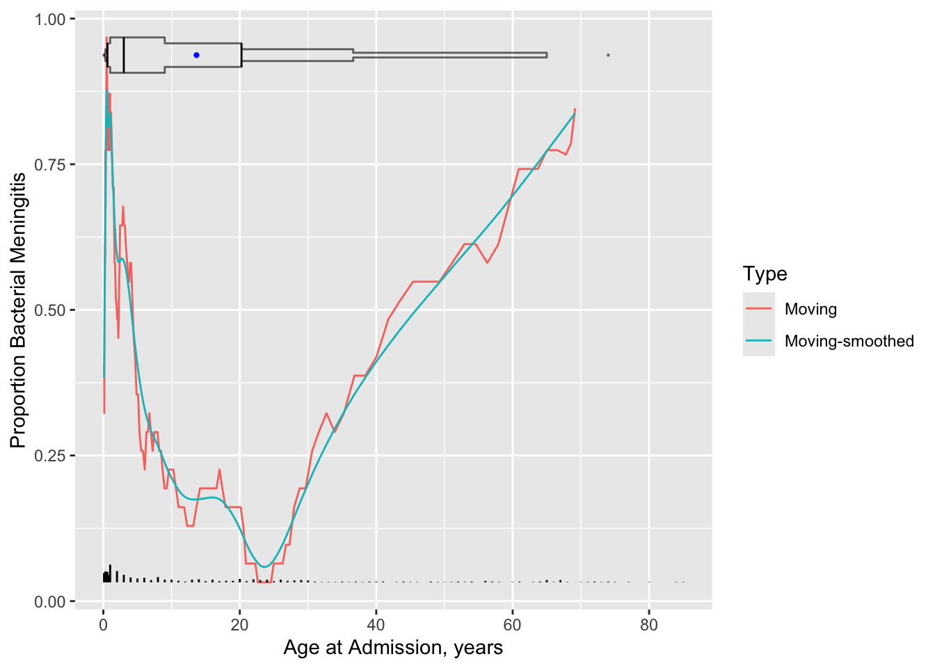
* Age example
```{r results='asis'}
#| label: fig-corr-age-abmm
#| fig-cap: 'Moving proportions relating age to the probability of bacterial meningitis given a patient has bacterial or viral meningitis, with a spike histogram and an extended box plot showing the age distribution. Moving proportions before smoothing are also shown. To the right of the extended box plot is a dot for the 0.99 quantile of age'
#| fig-scap: "Moving proportions"
require(qreport)   # provides addggLayers
u <- movStats(abm ~ age, msmooth='both', data=ABM, melt=TRUE, pr='margin')
g <- ggplot(u, aes(x=age, y=abm)) + geom_line(aes(col=Type)) +
  xlab('Age at Admission, years') +
  ylab('Proportion Bacterial Meningitis')
g <- addggLayers(g, ABM, value='age', type='spike')
addggLayers(g, ABM, value='age', type='ebp', pos='top')
```
* We also need to estimate the relationship between continuous variables and time-to-event when follow-up is incomplete
* Example: [VA lung cancer dataset](https://onlinelibrary.wiley.com/doi/book/10.1002/9781118032985)
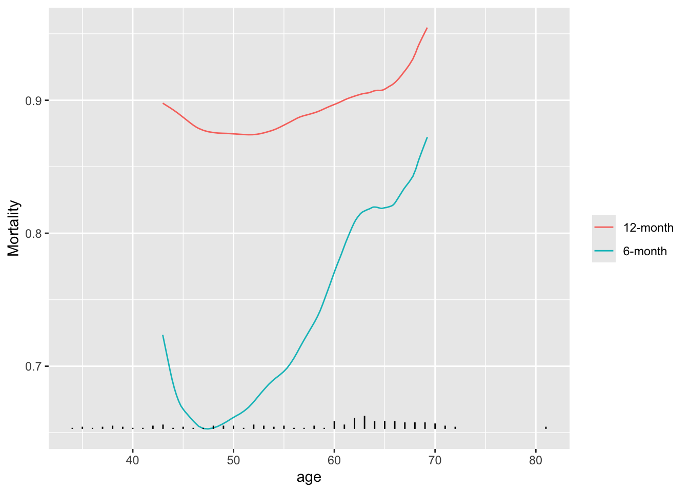
* For each moving window compute the Kaplan-Meier 6m and 12m survival estimates
* Subtract cumulative survival from 1.0 to get cumulative incidence
```{r results='asis'}
#| label: fig-corr-movsurv
#| fig-cap: "Moving 6m and 12m mortality as a function of age using VA lung cancer dataset"
#| fig-scap: "Moving 6m and 12m mortality estimates"
getHdata(valung)
require(survival)    # for Surv()
u <- movStats(Surv(t / (365.25 / 12), dead) ~ age, times=c(6, 12),
              eps=25, data=valung, melt=TRUE, pr='margin', tunits='month')
g <- ggplot(u, aes(x=age, y=incidence)) + geom_line(aes(col=Statistic)) +
      guides(color=guide_legend(title='')) + ylab('Mortality')
addggLayers(g, valung, value='age', type='spike')
```
```{r echo=FALSE}
saveCap('08')
```