```{r setup, include=FALSE}
require(Hmisc)
require(qreport)
hookaddcap() # make knitr call a function at the end of each chunk
# to try to automatically add to list of figure
options(prType='html')
getRs('qbookfun.r')
knitr::set_alias(w = 'fig.width', h = 'fig.height',
cap = 'fig.cap', scap ='fig.scap')
```
# Statistical Inference
`r mrg(abd("6"), bmovie(4), ddisc(4))`
## Overview
* Inferential modes
+ hypothesis testing
+ relative model fit/relative support for hypotheses (likelihood ratios, Bayes factors)
+ estimation (including interval estimation; often more appropriate than hypothesis testing)
+ Bayesian probability of an effect in the right direction (more relevant to decision making; more actionable)
* Contrast inference with decision making:
+ acting _as if something is true_ whether or not it is actually true
* Hypothesis testing is most useful for inferential "existence" questions
+ is indirect for other types of questions
* Majority of hypothesis tests are on a single point
* These place asymmetric importance on "special values" such as zero treatment effect
* What does it mean to "not reject a hypothesis"?
+ often very little
* What does it mean to reject a hypothesis with a statistical test?
+ in statistics it means that _some_ aspect of a model is under suspicion (e.g., normality assumption)
+ even if all other assumptions of the data model are satisfied, when the hypothesis involves a single point (e.g. zero effect), the alternative space is infinite so what have we learned about a _specific_ alternative (e.g., that a treatment lowers blood pressure by 10 mmHg)?
Statistical hypothesis testing involves a model for data:
* Parametric tests have very specific models
* Nonparametric tests have semi-specific models without a distribution assumption
* Permutation tests make an assumption about the best data summarization (e.g., mean, and the mean may not be the best summary for a heavy-tailed data distribution)
This chapter covers parametric tests for the following reasons:
1. historical
1. they are very useful for sample size estimation
1. occasionally one has prior information that the raw data, or differences from pre to post, actually follow a normal distribution, and with large effects one can get quite significant results in very small samples with parametric tests
1. to show that Bayesian parametric tests make fewer assumptions about the data model
Nonparametric methods are covered in Chapter @sec-nonpar.
Back to data model---the primary basis for statistical inference:
* Assume a model for how the data were generated
* Model contains
+ main parameters of interest (e.g., means)
+ auxiliary parameters for other variables (e.g., confounders)
+ parameters for sources of between-subject variability
+ if parametric, a distribution function such as Gaussian (normal)
+ if nonparametric/semiparametric, a connection between distributions for different types of subjects (link function)
+ if longitudinal, a correlation pattern for multiple measurements within a subject
+ assumptions about censoring, truncation, detection limits if applicable
+ ...
* Example (2-sample $t$-test): $Y = \mu_{0} + \delta [\textrm{treatment B}] + \epsilon$
+ $\mu_{0}$: unknown data-generating mean for treatment A
+ $\delta$: unknown data-generating difference in means (B-A)
+ $[\textrm{treatment B}]$: an indicator variable (1 if observation is from treatment B, 0 if from treatment A)
+ $\epsilon$: irreducible error, i.e., unaccountable subject-to-subject variation; biologic variability; has variance $\sigma^2$
+ **Primary goal**: uncover the hidden value of $\delta$ generating our dataset in the presence of noise $\epsilon$
- higher $\sigma^{2} \rightarrow$ larger $|\epsilon| \rightarrow$ harder to uncover $\delta$ (the signal) from the noise
- were $\epsilon$ always zero (no uncertainties), one _directly observes_ $\delta$ and no statistical analysis is needed
* Rejecting a straw-man hypothesis implies that _some_ aspect of the model is in doubt
+ that aspect may be the distribution or an assumption about equal variances, not the difference in means you care about
**Common error**: Using a two-stage approach to select which data
model to use:
* Assumes the data contain rich enough information to lead to a correct decision
* Alters the operating characteristics of the final test
* Fails to realize that nonparametric tests have excellent power
Example: Testing normality to decide on whether to use a $t$-test
vs. a Wilcoxon-Mann-Whitney two-sample rank test. A two-stage test
with a test for normality in the first stage assumes that
1. the test for normality has power near 1.0 for our sample size
1. if the test rejects $H_{0}$:normality, the magnitude of non-normality is worth bothering about
1. pre-testing for normality does not modify the type I error of the overall testing procedure
1. nonparametric tests are less efficient than parametric tests
In fact it may be that none of these assumptions is true (4. is very seldom true). As will be
seen later, a full Bayesian model can be completely honest and provide
exactly the right amount of caution:
* flexible parametric model allowing uncertainty about equal variances for groups A and B
* allows uncertainty about the normality assumption
* still results in inference about $\delta$, properly more cautious (wider credible interval) because
+ we don't know if normality truly holds
+ we don't know if equality of variance truly holds
### Central Limit Theorem
`r quoteit('The CLT is frequently misunderstood by practitioners when they use a limit theorem on their finite data to compute falsely symmetric confidence intervals. Asymmetric data must lead to asymmetric confidence intervals, otherwise confidence coverage will be inaccurate in at least one of the two tails. When the SD is unknown and must be estimated from the data, practitioners assume that the SD is a good measure of dispersion (it isn\'t, for asymmetric or heavy-tailed distributions) and the CLT assumes the mean and SD are uncorrelated (they aren\'t, for asymmetric distributions). An example where things go terribly wrong is when you should have taken logs but didn\'t.')`
The essence of the CLT is
* Assume observations are independent with the same distribution and have finite variance
* Assume that the sample size $n$ can increase without bound
* Limiting distribution of the sample mean is normal
The CLT is frequently used to justify the use of parametric
statistical tests and confidence intervals even when their assumptions
are violated. **But** the CLT (and the $t$ distribution) are
much less helpful for computing confidence intervals and $P$--values
than it seems @wil13avo:
* since the standard deviation is unknown, one must estimate it while estimating the mean to use the CLT
* SD may be a completely inappropriate summary of dispersion (e.g., if one should have first log-transformed but computed SD on the raw scale)
* if the data distribution is asymmetric, the SD is not independent of the mean (so the $t$ distribution does not hold) and the SD is not a good dispersion measure
* the sample size for which the CLT is an adequate approximation is unknown for any given situation
* example: log-normal distribution---the CLT is not accurate even for $n=50000$ (see below)
* even when the CLT provides somewhat accurate $P$-values, it provides no comfort with regard to statistical power. Example: analyzing $Y$ when you should have analyzed $\log(Y)$ will result in a devastating increase in type II error.
Example simulation to compute confidence-coverage when using the
$t$-distribution confidence interval for $n=50,000$ when analyzing
data from a log-normal distribution but not taking logs. We want the
confidence limits to be such that the fraction of samples for which
the true population mean is to the left of the lower limit is 0.025,
and the fraction to the right of the upper limit to also be 0.025.[For more about `runifChanged` go [here](http://hbiostat.org/rflow/caching.html). The way `runifChanged` is used below, the results are stored in a file whose name is the name of the `Quarto/knitr` chunk followed by `.clt`.]{.aside}
```{r clt}
n    <- 50000
nsim <- 5000            # number of simulations
mul <- 0; sdl <- 1.65   # on log scale
mu <- exp(mul + sdl * sdl / 2)   # population mean on orig. scale
count <- c(lower=0, upper=0)
seed <- 1
set.seed(seed)
z <- qt(0.975, n - 1)   # t critical value (near 1.96)

g <- function() {
  for(i in 1 : nsim) {
    x <- exp(rnorm(n, mul, sdl))
    ci <- mean(x) + c(-1, 1) * z * sqrt(var(x) / n)
    count[1] <- count[1] + (ci[1] > mu)
    count[2] <- count[2] + (ci[2] < mu)
  }
    count / nsim  # non-coverage prob. in left and right tails
}
f <- runifChanged(g, n, nsim, mul, sdl, seed, z)  # runifChanged in Hmisc
as.vector(f)   # should be 0.025 0.025 if CLT is accurate
```
See
[stats.stackexchange.com/questions/204585](https://stats.stackexchange.com/questions/204585) and [here](https://stats.stackexchange.com/questions/608740) for more information and discussion.
## Hypotheses
### Scientific Hypotheses and Questions
Scientific questions are usually stated with a direction or with
regard to an expected effect, not with respect to a null effect.
Scientific questions often involve estimating a quantify of interest.
Here are some examples:
* Does the risk of death increase when serum triglyceride increases?
* To what extent is mechanism $x$ responsible for regulation of physiologic parameter $y$?
* What is the average decrease in blood pressure when the dose of a drug goes from 0 to 10mg/day to 20mg/day?
### Statistical Hypotheses
* Hypothesis: usually a statement to be judged of the form <br> "population value = specified constant"
+ $\mu = 120$mmHg
+ $\mu_{1} - \mu_{2} = 0$mmHg
+ Correlation between wealth and religiosity = 0
* Null hypothesis is usually a hypothesis of no effect but can be $H_{0}: \mu =$ constant or $H_{0}:$ Probability of heads $=\frac{1}{2}$; <br> $H_{0}$ is often a straw man; something you hope to disprove
* Alternative hypothesis: $H_1$; e.g.: $H_{1}: \mu \neq 120$mmHg
* One-sided hypothesis (tested by 1-tailed test): $H_{1}$ is an inequality in one direction ($H_{1}: \mu > 120$mmHg)
* Two-sided hypothesis (2-tailed test, most common type): $H_{1}$ involves values away from the hypothesized value in either direction
## Branches of Statistics {#sec-htest-branches}
* Classical (frequentist or sampling statistics)
+ Emphasizes (overemphasizes?) hypothesis testing
+ Assumes $H_{0}$ is true and tries to amass evidence casting doubt on this assumption
+ Conceives of data as one of many datasets that _might_ have happened; considers the process by which the sample arose
+ Inference is based on long-run operating characteristics not about direct evidence from the sample at hand
- probability of making an assertion of an effect if there is no effect
- proportion of the time that varying confidence intervals over replicates of the experiment cover the true unknown parameter; no statement about the chance that the current confidence interval covers the true parameter
+ See if data are consistent with $H_{0}$
+ Are data extreme or unlikely if $H_{0}$ is really true?
+ Proof by contradiction: if assuming $H_{0}$ is true leads to results that are "bizarre" or unlikely to have been observed, casts doubt on premise
+ Evidence summarized through a single statistic capturing a tendency of data, e.g., $\bar{x}$
+ Look at probability of getting a statistic as or more extreme than the calculated one (results as or more impressive than ours) if $H_{0}$ is true (the $P$-value)^[We could drop the "as" and just say "more extreme" because for continuous data the probability of getting a result exactly as extreme as ours is exactly zero.]
+ If the statistic has a low probability of being more extreme we say that if $H_{0}$ is true we have acquired data that are very improbable, i.e., have witnessed a low probability event
+ [William Briggs](https://wmbriggs.com/public/Briggs.EverthingWrongWithPvalues.pdf) described a basic flaw in the logic of $P$-value-guided hypothesis testing dating all the way back to Fisher:
`r quoteit('A version of an argument given first by Fisher appears in every introductory statistics book. The original argument is this, [33]:<br><br>"Belief in a null hypothesis as an accurate representation of the population sampled is confronted by a logical disjunction: Either the null hypothesis is false, or the p-value has attained by chance an exceptionally low value."<br><br> A logical disjunction would be a proposition of the type "Either it is raining or it is not raining." Both parts of the proposition relate to the state of rain. The proposition "Either it is raining or the soup is cold" is a disjunction, but not a logical one because the first part relates to rain and the second to soup. Fisher\'s "logical disjunction" is evidently not a logical disjunction because the first part relates to the state of the null hypothesis and the second to the p-value. Fisher\'s argument can be made into a logical disjunction, however, by a simple fix. Restated: Either the null hypothesis is false and we see a small p-value, or the null hypothesis is true and we see a small p-value. Stated another way, "Either the null hypothesis is true or it is false, and we see a small p-value." The first clause of this proposition, "Either the null hypothesis is true or it is false", is a tautology, a necessary truth, which transforms the proposition to (loosely) "TRUE and we see a small p-value." Adding a logical tautology to a proposition does not change its truth value; it is like multiplying a simple algebraic equation by 1. So, in the end, Fisher\'s dictum boils down to: "We see a small p-value." In other words, in Fisher\'s argument a small p-value has no bearing on any hypothesis (any hypothesis unrelated to the p-value itself, of course). Making a decision about a parameter or data because the p-value takes any particular value is thus always fallacious: it is not justified by Fisher\'s argument, which is a non sequitur.', 'William Briggs')`
* Ignoring all that and plunging ahead:
+ $P$-value is a measure of _surprise_ that is well described by Nicholas Maxwell^[Data Matters: Conceptual Statistics for a Random World. Emeryville CA: Key College Publishing, 2004.]: "A p value is a measure of how embarrassing the data are to the null hypothesis"
+ Then evidence mounts against $H_{0}$ and we might reject it
+ A failure to reject _does not_ imply that we have gathered evidence in favor of $H_0$ --- many reasons for studies to not be impressive, including small sample size ($n$)
+ Ignores _clinical_ significance
+ Is fraught with how to deal with multiplicity problems
- No principled recipe for how they should be handled
- Arise because<br>type I error is fixed at a number $> 0$<br>backward time ordering of information (transposed conditional)
- Evidence about one question is changed according to whether other questions are asked (regardless of their answers)
* Classical parametric statistics: assumes the data to arise from a certain distribution, often the normal (Gaussian distribution)
* Nonparametric statistics: does not assume a data distribution; generally looks at ranks rather than raw values
* Bayesian statistics:
+ Considers the sample data, not how it arose from a sequence of samples but rather the data generating mechanism for _this_ sample
+ Computes the probability that a clinically interesting statement is true, e.g. that the new drug lowers population mean SBP by at least 5mmHg, given what we observed in the data
+ Instead of trying to amass evidence against a single hypothesized effect size, Bayes tries to uncover the hidden parameter generating the data aside from noise (e.g., treatment effect) whatever its value
- Provides evidence for _all possible values_ of an unknown parameter
+ More natural and direct approach but requires more work
+ Because respects forward flow of time/information there is no need for nor availability of methods for correcting for multiplicity^[Bayesian inference assumes only that the prior distribution is "well calibrated" in the sense that one sticks to the pre-specified prior no matter what information is unveiled.]
+ Evidence about one question is not tilted by whether other questions are asked
+ Can formally incorporate knowledge from other studies as well as skepticism from a tough audience you are trying to convince to use a therapy
+ Starting to catch on (only been available for about 240 years) and more software becoming available
* Likelihood inference^[A key thinker and researcher in the field is Richard Royall.]:
+ Considers the sample data, not how it arose
+ Akin to Bayesian but without the prior
+ Interval estimates are based on relative likelihood (from the likelihood function) and are called likelihood support intervals
+ For testing, allows both type I and type II errors $\rightarrow 0$ as $n \rightarrow \infty$, whereas with frequentist methods the type I error never shrinks as $n \rightarrow \infty$
+ This greatly reduces problems with multiplicities
+ Likelihood methods do not deal well with complex assertions (e.g., either the treatment reduces mortality by any amount or reduces blood pressure by at least 10 mmHg) and do not allow the use of external information
* Bayesian and likelihood inference use the _likelihood principle_; frequentist inference does not
+ Likelihood principle: All of the evidence in a sample relevant to model parameters is in the likelihood function
+ If we want to know our current location, frequentist inference asks the following: If I am in Nashville, what fraction of routes to here involved the southern route I took? There are many paths to get where we are, and frequentists have to consider all possible relevant paths. Bayesian and likelihood inference states it differently: Where am I now? This involves an assessment of current evidence about my location. Asking "how did I get here?" (i.e., how did the data arise?) involves multiplicity issues that answering the simpler question does not.
+ Consider a sequentially monitored randomized experiment. Bayesians and likelihoodists can make infinitely many assessments of efficacy with no penalty. On the other hand, a frequentist must think the following way:
`r quoteit('I am at the first interim analysis. I am going to make later assessments of efficacy so I need to discount the current assessment and be more conservative or I will spend all my $\\alpha$ already.<br>...<br>I am at the fifth interim analysis. I made four previous efficacy assessments, and even though none of them mattered, because they _may have mattered_ I spent $\\alpha$ so I need to discount the current assessment and be more conservative.')`
* We will deal with classical parametric and nonparametric statistical tests more than Bayesian methods only because of time and because of abundance of easy-to-use software for the former
## Errors in Hypothesis Testing; $P$ Values
* Can attempt to reject a formal hypothesis or just compute $P$-value
* Type I error: rejecting $H_0$ when it is true <br> $\alpha$ is the probability of making this error (typically set at $\alpha=0.05$---for weak reasons)
+ To be specific: $\alpha$ = P(asserting an effect exists when in fact it doesn't)
+ So it is an assertion probability or false alarm probability like 1 minus specificity
+ It **is not** a false positive probability (P(effect=0) given an assertion that it is nonzero) since $\alpha$ is based on an **assumption** that effect=0
* Type II error: failing to reject $H_0$ when it is false <br> probability of this is $\beta$
| | True state of $H_0$ | |
|-----|-----|------|
| Decision | $H_0$ true | $H_0$ false |
| Reject $H_0$ | Type I error ($\alpha$) | Correct |
| Do Not Reject $H_0$ | Correct | Type II error ($\beta$) |
* Power: $1 - \beta$: probability of (correctly) rejecting $H_0$ when it is false
Within the frequentist framework of statistics there are two schools.
One, the Neyman-Pearson school, believes that the type I error should
be pre-set at $\alpha$ (say $\alpha=0.05$) so that binary decisions
can be made (reject/fail to reject). The other school due to Fisher
believes that one should compute $P$-values and quote the result in
the report or publication. This is the more popular approach, being less dichotomous.
* Simplest definition of $\alpha$: probability that a $P$-value will be less than it if the treatment is ignorable
A $P$-value is something that can be computed without speaking of
errors. It is the probability of observing a statistic as or more
extreme than the observed one if $H_0$ is true, i.e., if the
population from which the sample was randomly chosen had the
characteristics posited in the null hypothesis.^[Note that Rosner's Equation 7.4 in his section 7.3 is highly problematic. Classifications of "significant" or "highly significant" are arbitrary, and treating a $P$-value between 0.05 and 0.1 as indicating a "trend towards significance" is bogus. If the $P$-value is 0.08, for example, the 0.95 confidence interval for the effect includes a "trend" in the opposite (harmful) direction.] The $P$-value to have the usual meaning assumes that the data model is correct.
### Problems With Type I Error
* It's not really an "error"
+ Error = being wrong in asserting an effect
+ Type I = P(asserting effect $| H_{0}$) = "effect assertion probability"
* Frequentist designs attempt to preserve type I error
* This is not the probability of making a mistake in concluding an effect is present
* When $\alpha=0.05$ the probability of asserting an effect when there is none never decreases even as $n \rightarrow \infty$ <br> (statistical vs. clinical significance problem)
* $\alpha$ does not depend on any observed data. It is a pre-study concept.
* $\alpha$ increases because of chances you give data to be more extreme (multiplicity), not because of chances you give hypotheses to be false. Bayesian and likelihood approaches do not look at sampling (sample space giving rise to data extremes). See [this](https://fharrell.com/post/bayes-seq)
* Probability of making a mistake in asserting an effect, given
the data, is one minus the Bayesian posterior probability of efficacy
### Misinterpretation of $P$-values
$P$-values have come under extreme criticism since 2000, partially
because they are often misinterpreted. @gre16sta
is the best paper that summarizes the misinterpretations and explains
them. Some quotes from this paper are below, with their explanations
for the first two.
> 1. **The $P$ value is the probability that the test hypothesis is true; for example, if a test of the null hypothesis gave $P$ = 0.01, the null hypothesis has only a 1\% chance of being true; if instead it gave $P$ = 0.40, the null hypothesis has a 40\% chance of being true.** No! The $P$ value assumes the test hypothesis is true---it is not a hypothesis probability and may be far from any reasonable probability for the test hypothesis. The $P$ value simply indicates the degree to which the data conform to the pattern predicted by the test hypothesis and all the other assumptions used in the test (the underlying statistical model). Thus $P$ = 0.01 would indicate that the data are not very close to what the statistical model (including the test hypothesis) predicted they should be, while $P$ = 0.40 would indicate that the data are much closer to the model prediction, allowing for chance variation.
1. **The $P$ value for the null hypothesis is the probability that chance alone produced the observed association; for example, if the $P$ value for the null hypothesis is 0.08, there is an 8\% probability that chance alone produced the association.** No! This is a common variation of the first fallacy and it is just as false. To say that chance alone produced the observed association is logically equivalent to asserting that every assumption used to compute the $P$ value is correct, including the null hypothesis. Thus to claim that the null $P$ value is the probability that chance alone produced the observed association is completely backwards: The $P$ value is a probability computed assuming chance was operating alone. The absurdity of the common backwards interpretation might be appreciated by pondering how the $P$ value, which is a probability deduced from a set of assumptions (the statistical model), can possibly refer to the probability of those assumptions. Note: One often sees "alone" dropped from this description (becoming "the $P$ value for the null hypothesis is the probability that chance produced the observed association"), so that the statement is more ambiguous, but just as wrong.
1. **A significant test results ($P\leq 0.05$) means that the test hypothesis is false or should be rejected.** No!
1. **A nonsignificant test results ($P > 0.05$) means that the test hypothesis is true or should be accepted.** No!
1. **A large $P$ value is evidence in favor of the test hypothesis.** No!
1. **A null-hypothesis $P$ value greater than 0.05 means that no effect was observed, or that absence of an effect was shown or demonstrated.** No!
1. **Statistical significance indicates a scientifically or substantively important relation has been detected.** No!
1. **Lack of statistical significance indicates that the effect size is small.** No!
1. **The $P$ value is the chance of our data occurring if the test hypothesis is true; for example, $P$ = 0.05 means that the observed association would occur only 5\% of the time under the test hypothesis.** No!
1. **If you reject the test hypothesis because $P \leq 0.05$, the change you are in error (the chance your "significant finding" is a false positive) is 5\%.** No!
1. **$P = 0.05$ and $P \leq 0.05$ mean the same thing.** No!
1. **$P$ values are properly reported as inequalities (e.g., report "$P < 0.02$" when $P = 0.015$ or report $P > 0.05$ when $P = 0.06$ or $P = 0.70$).** No!
1. **Statistical significance is a property of the phenomenon being studied, and thus statistical tests detect significance.** No!
1. **One should always use two-sided $P$ values.** No!
1. **When the same hypothesis is tested in different studies and none or a minority of the tests are statistically significant (all $P > 0.05$), the overall evidence supports the hypothesis.** No!
1. **When the same hypothesis is tested in two different populations and the resulting $P$ values are on opposite sides of 0.05, the results are conflicting.** No!
1. **When the same hypothesis is tested in two different populations and the same $P$ values are obtained, the results are in agreement.** No!
1. **If one observes a small $P$ value, there is a good chance that the next study will produce a $P$ value at least as small for the same hypothesis.** No!
1. **The specific 95\% confidence interval presented by a study has a 95\% chance of containing the true effect size.** No!
1. **An effect size outside the 95\% confidence interval has been refuted (or excluded) by the data.** No!
1. **If two confidence intervals overlap, the difference between the two estimates or studies is not significant.** No!
1. **An observed 95\% confidence interval predicts that 95\% of the estimates from future studies will fall inside the observed interval.** No!
1. **If one 95\% confidence interval includes the null value and another excludes that value, the interval excluding the null is the more precise one.** No!
1. **If you accept the null hypothesis because the null $P$ value exceeds 0.05 and the power of your test is 90\%, the chance you are in error (the chance that your finding is a false negative) is 10\%.** No!
1. **If the null $P$ value exceeds 0.05 and the power of this test is 90\% at an alternative, the results support the null over the alternative.** \dots counterexamples are easy to construct \dots
## Interval Estimation
### Frequentist Confidence Intervals
A $1-\alpha$ two-sided confidence interval is an interval computed such that
* if the experiment were repeated $N$ times one would expect $N \times (1 - \alpha)$ of the recomputed varying intervals to contain the true unknown quantity of interest
* equivalently the set of all unknown population parameter values that if null hypothesized one would not reject that null hypothesis at the $\alpha$ level in a two-sided test
+ e.g. when estimating the population mean $\mu$, the set $\mu_{0}$ such that the test $H_{0}: \mu = \mu_{0}$ has a $P$-value $> \alpha$
For this reason confidence intervals may better be called _compatibility intervals_.
**Pros**:
* The $P$-value can be computed from the confidence interval but not vice-versa, so confidence limits have more information
* Confidence intervals do not allow the "absence of evidence is not evidence of absence error"
+ large $P$-values can come from small $n$ or large $\sigma^2$
+ these make confidence intervals wide, giving a rational sense of uncertainty
+ A confidence interval that is compatible with both large benefit and large detriment indicates that we don't know much
- large $P$-value means nothing more than "get more data"
**Cons**:
* Confidence intervals have only a long-run interpretation over many experiments
* They don't provide a probability statement about whether a single interval includes the true population value
+ In the frequentist world, the probability that the parameter is in a given interval is either zero or one
* They are often taken to provide a measure of precision of a statistical estimate, but they're not really that either
* The experimenter controls the long-run inclusion probability $1 - \alpha$ and gets interval endpoints, but is often more interested in the probability that the population effect is in a pre-chosen fixed interval
* It is very difficult to make confidence intervals incorporate known uncertainties (e.g., amount of non-normality), making them often too narrow (overoptimistic)
### Bayesian Credible Intervals
* Credible intervals have the interpretation that most researchers seek when they compute confidence intervals
* A $1 - \alpha$ credible interval is an interval $[a, b]$ (computed, under a certain prior distribution encapsulating prior knowledge about the parameter $\mu$) so that <br> $P(a \leq \mu \leq b | \textrm{ data}) = 1 - \alpha$
**Pros**:
* Pertains to the single, current dataset and does not provide just long-run operating characteristics
* Provides a true probability statement even when the experiment could never be repeated
* Is symmetric with Bayesian posterior probabilities of pre-chosen limits
+ Researchers can specify $a, b$ and then compute whatever probability it is that the unknown parameter is in that interval
* The credible interval can take into account all sorts of uncertainties (e.g., non-normality) that make it (correctly) wider
**Cons**:
* One must specify a prior distribution
## One Sample Test for Mean
`r mrg(bmovie(5), ddisc(5))`
### Frequentist Method
* Assuming continuous response from a normal distribution
* One sample tests for $\mu =$ constant are unusual except when data are paired, e.g., each patient has a pre-- and post--treatment measurement and we are only interested in the mean of post - pre values
* $t$ tests in general:
$$t = \frac{\text{estimate - hypothesized value}}{\text{standard deviation of numerator}} $$
* The standard deviation of a summary statistic is called its _standard error_, which is the $\sqrt{}$ of the variance of the estimate
* The one-sample $t$ statistic for testing a single population mean against a constant $\mu_0$ ($H_{0}$: $\mu = \mu_{0}$; often $\mu_{0} = 0$) is
$$
t = \frac{\bar{x} - \mu_{0}}{se}
$$
where $se = \frac{s}{\sqrt{n}}$, is the standard error of the mean (SEM) and $\bar{x}$ is the sample mean
<!-- because the variance of $\bar{x}$ is the variance of an individual $x$ value divided by the number of values being averaged $\rightarrow \sigma^{2}/n$--->
<!-- \bi--->
<!-- * If you repeated an experiment $M$ times, each time computing--->
<!-- $\bar{x}$ from $n$ observations, the $M \bar{x}$s would vary--->
<!-- $\frac{1}{n}$th as much as the raw measurements vary between--->
<!-- patients--->
<!-- \ei--->
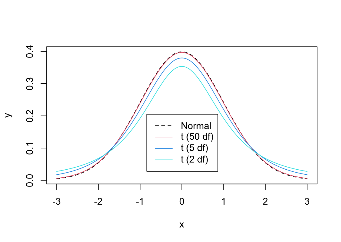
* When your data comes from a normal distribution and $H_{0}$ holds, the $t$ ratio **statistic** follows the $t$ **distribution**
* With small sample size ($n$), the $t$ ratio is unstable because the sample standard deviation ($s$) is not precise enough in estimating the population standard deviation ($\sigma$; we are assuming that $\sigma$ is unknown)
* This causes the $t$ distribution to have heavy tails for small $n$
* As $n\uparrow$ the $t$ distribution becomes the normal distribution with mean zero and standard deviation one
* The parameter that defines the particular $t$ distribution to use as a function of $n$ is called the _degrees of freedom_ or d.f.
* d.f. = $n$ - number of means being estimated
* For one-sample problem d.f. = $n-1$
* Symbol for distribution $t_{n-1}$
```{r tpdfs,w=6,h=4.25,cap='Comparison of probability densities for $t_2$, $t_5$, $t_{50}$, and normal distributions',scap='$t$ distribution for varying d.f.'}
#| label: fig-htest-tpdfs
x <- seq(-3, 3, length=200)
w <- list(Normal     = list(x=x, y=dnorm(x)),
          't (50 df)'= list(x=x, y=dt(x, 50)),
          't (5 df)' = list(x=x, y=dt(x, 5)),
          't (2 df)' = list(x=x, y=dt(x,2)))
labcurve(w, pl=TRUE, keys='lines', col=c(1,2,4,5), lty=c(2,1,1,1),
         xlab=expression(x), ylab='')
```
* Two-tailed $P$-value: probability of getting a value from the $t_{n-1}$ distribution as big or bigger in absolute value than the absolute value of the observed $t$ ratio
* Computer programs can compute the $P$-value given $t$ and $n$.^[`R` has the function <tt>pt</tt> for the cumulative distribution function for the $t$ distribution, so the 2-tailed $P$-value would be obtained using <tt>2*(1-pt(abs(t),n-1))</tt>.] `R` can compute all probabilities or critical values of interest. See the help files for `pt,pnorm,pf,pchisq`.
<!-- See the course web site or go--->
<!-- to [surfstat.anu.edu.au/surfstat-home/tables/t.php](http://surfstat.anu.edu.au/surfstat-home/tables/t.php) for--->
<!-- an interactive $P$ and critical value calculator for common--->
<!-- distributions.--->
+ don't say "$P <$ something" but instead $P=$ something
* In the old days tables were used to provide _critical values_ of $t$, i.e., a value $c$ of $t$ such that Prob$[|t| > c] = \alpha$ for "nice" $\alpha$ such as 0.05, 0.01.
* Denote the critical value by $t_{n-1;1-\alpha/2}$ for a 2-tailed setup
* For large $n$ (say $n \geq 500$) and $\alpha=0.05$, this value is almost identical to the value from the normal distribution, 1.96
* Example: We want to test if the mean tumor volume is 190 mm$^3$ in a population with melanoma, $H_0: \mu = 190$ versus $H_1: \mu \neq 190$.
$$\begin{array}{c}
\bar{x}=181.52, s=40, n=100, \mu_{0}=190 \\
t = \frac{181.52 - 190}{40/\sqrt{100}} = -2.12 \\
t_{99,.975}=1.984 \rightarrow \mathrm{reject~at~arbitrary~\alpha=.05~if~using~Neyman-Pearson~paradigm} \\
P=0.037
\end{array}$$
```{r tone}
xbar  <- 181.52
s     <- 40
n     <- 100
mu0   <- 190
tstat <- (xbar - mu0) / (s / sqrt(n))
pval  <- 2 * (1 - pt(abs(tstat), n - 1))
c(tstat=tstat, pval=pval)
```
### Bayesian Methods
* All aspects of Bayesian probabilistic inference follow from the general form of Bayes' rule allowing for the response $Y$ to be continuous:<br>The probability density function for the unknown parameters given the data and prior is proportional to the density function for the data multiplied by the density function for the prior^[When $Y$ is a discrete categorical variable we use regular probabilities instead of densities in Bayes' formula. The density at $x$ is the limit as $\epsilon \rightarrow 0$ of the probability of the variable being in the interval $[x, x + \epsilon]$ divided by $\epsilon$.]
* The Bayesian counterpart to the frequentist $t$-test-based approach can use the same model
* But brings extra information for the unknowns---$\mu, \sigma$---in the form of prior distributions for them
* Since the raw data have a somewhat arbitrary scale, one frequently uses nearly flat "weakly-informative" priors for these parameters
+ But it would be easy to substitute a prior for $\mu$ that rules out known-to-be impossible values or that assumes very small or very large $\mu$ are very unlikely
* **Note**: the assumption of a Gaussian distribution for the raw data $Y$ is a strong one
+ Bayes makes it easy to relax the normality assumption but still state the inference in familiar terms (e.g., about a population mean)^[Some analysts switch to trimmed means in the presence of outliers but it is hard to interpret what they are estimating.]
+ See later for an example
* For now assume that normality is known to hold, and use relatively uninformative priors
\head{Bayesian Software}
In most Bayesian analyses that follow we use the `R`
`brms` package by Paul-Christian Bürkner that is based on the
general [Stan](http://mc-stan.org) system because `brms` is easy to
use, makes good default choices for priors, and uses the same
notation as used in frequentist models in `R`footnote{Thanks to Nathan James of the Vanderbilt Department of Biostatistics for providing `brms` code for examples in this chapter.}.
Except for the one-sample proportion example in the next section, our
Bayesian calculations are general and do not assume that the posterior
distribution has an analytic solution. Statistical samplers (Markov
chain Monte Carlo, Gibbs, and many variants) can sample from the
posterior distribution only by knowing the part of Bayes' formula that
is the simple product of the data likelihood and the prior, without
having to integrate to get a marginal distribution^[The simple product is proportional to the correct posterior distribution and just lacks a normalizing constant that makes the posterior probabilities integrate to 1.0.]. We are generating
4000 samples from the posterior distribution (4000 random draws) in
this chapter. When high precision of posterior probabilities is
required, one can ensure that all probability calculations have a
margin of simulation error of $< 0.01$ by using 10,000 samples, or
margin of error $< 0.005$ by taking 40,000 draws^[These numbers depend on the sampler having converged and the samples being independent enough so that the number of draws is the effective sample size. `Stan` and `brms` have diagnostics that reveal the effective sample size in the face of imperfect posterior sampling.].
**Example**
To introduce the Bayesian treatment for the one-sample continuous $Y$
problem consider the following made-up dataset that has an "outlier":
98 105 99 106 102 97 103 132
* Start with regular frequentist analysis
* Most interested in confidence interval
* Also test $H_{0}: \mu = 110$
Five measures of dispersion are computed^[In a standard normal(0,1) distribution, the measures are, respectively, 1.0, 0.8, 0.8, 1.13, and 0.67.].
```{r freqex}
y <- c(98, 105, 99, 106, 102, 97, 103, 132)
median(y)
sd(y)
mean(abs(y - mean(y)))
mean(abs(y - median(y)))
GiniMd(y) # Gini's mean difference is more robust to outliers
 # It is the mean absolute difference over all pairs of observations
median(abs(y - median(y)))   # Even more robust, not as efficient
t.test(y, mu=110)
```
Now consider a Bayesian counterpart. A one-sample problem is a linear
model containing only an intercept, and the intercept represents the
overall unknown data-generating (population) mean of $Y$. In `R` an intercept-only model has <tt>~ 1</tt> on
the right-hand side of the model formula.
For the prior distribution for the mean we assume a most likely value (mean of distribution, since symmetric) of 150 and a standard deviation of 50, indicating the unknown mean is likely to be between 50 and 250. This is a weakly informative prior.
```{r bayesex0,cache=FALSE}
# Tell brms/Stan/rstanarm to use all available CPU cores except for 1
options(mc.cores=parallel::detectCores() - 1)
```
```{r bayesex,results='none'}
require(brms)
d <- data.frame(y)
priormu <- prior(normal(150,50), class='Intercept')
h <- function() brm(y ~ 1, family=gaussian, prior=priormu, data=d, seed=1)
f <- runifChanged(h, priormu, d)
```
See which prior distributions are being assumed. The data model is
Gaussian. Also display parameter distribution summaries.
`Estimate` represents the mean of the posterior distribution.
```{r bayesex2}
prior_summary(f)
f
draws <- as.data.frame(f)
mu    <- draws$b_Intercept
sigma <- draws$sigma
length(mu)
```
* Note how Bayes provides uncertainty/precision information about $\sigma$
* Credible intervals are quantiles of posterior samples, e.g. we can duplicate the above credible interval (`CI`) for $\mu$ (the intercept) using the following:
```{r quantci}
quantile(mu, c(.025, 0.975))
```
* Compare 0.95 credible interval with the 0.95 frequentist confidence interval above
* Compare posterior means for $\mu, \sigma$ with the point estimates from the traditional analysis
+ Posterior modes (the most likely values) may be more relevant^[The sample mean is the maximum likelihood estimate (MLE) and the sample standard deviation is, except for a factor of $\frac{n-1}{n}$, the maximum likelihood estimate. When priors are flat, MLEs equal posterior modes]. These are printed below along with sample estimates. The posterior mode is computed by fitting a nonparametric kernel density estimator to the posterior draws for the parameter of interest and finding the peak. The number of draws needed to compute the mode accurately is more than the number we are using here.
```{r modemsd}
# Function to compute posterior mode given draws
pmode <- function(x) {
  z <- density(x)
  z$x[which.max(z$y)]
  }
n <- length(y)
c(mean(y), sd(y), sd(y)*sqrt((n-1)/n))
c(pmode(mu), pmode(sigma))
```
* Instead of a hypothesis test we compute direct evidence for $\mu$ exceeding 110
+ posterior probability that $\mu > 110$ given the data and priors is approximated (to within simulation error) by the proportion of posterior draws for $\mu$ for which the value of $\mu$ exceeded 110
+ define a "probability operator" `P` that is just the proportion
```{r bayesex3}
P <- mean
P(mu > 110)   # compare to 1-tailed p-value: 0.136
```
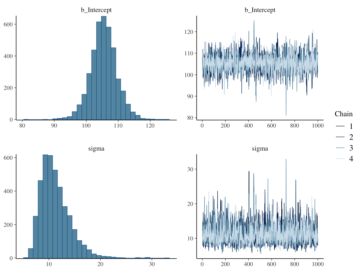
Here are posterior distributions for the two parameters along with
convergence diagnostics
```{r bayesex4,h=6,w=8,cap="Posterior distributions for $\\mu$ and $\\sigma$ using a normal data model with weak priors (left panels), and convergence diagnostics for posterior sampling (right panels)",scap="Posterior distributions for $\\mu$ and $\\sigma$ using a normal model."}
#| label: fig-htest-bayesex4
plot(f)
```
* Normality is a strong assumption
* Heavy tails can hurt validity of the estimate of the mean, uncertainty intervals, and $P$-values
* Easy to allow for heavy tails by adding a single parameter to the model^[One could use a data distribution with an additional parameter that allows for asymmetry of the distribution. This is not addressed here.]
* Assume the data come from a $t$ distribution with unknown degrees of freedom $\nu$
+ Use of $t$ for the raw data distribution should not be confused with the use of the same $t$ distribution for computing frequentist probabilities about the sample mean.
+ John Kruschke has championed this Bayesian $t$-test approach in [BEST](https://cran.r-project.org/web/packages/BEST/vignettes/BEST.pdf) (Bayesian Estimation Supersedes the $t$-Test)
* $\nu > 20 \rightarrow$ almost Gaussian
* Have a prior for $\nu$ that is a gamma distribution with parameters $\alpha=2, \beta=0.1$ with $\nu$ constrained to be $> 1$
* Prior $P(\nu > 20)$ is (in `R` code) `pgamma(20,2,0.1,lower.tail=FALSE)` which is `r round(pgamma(20,2,0.1,lower.tail=FALSE), 2)`. So our prior probability that normality approximately holds is a little less than $\frac{1}{2}$.
```{r bayesext1,results='none'}
h <- function() brm(y ~ 1, family=student, prior=priormu, data=d, seed=2)
g <- runifChanged(h, priormu, d)
```
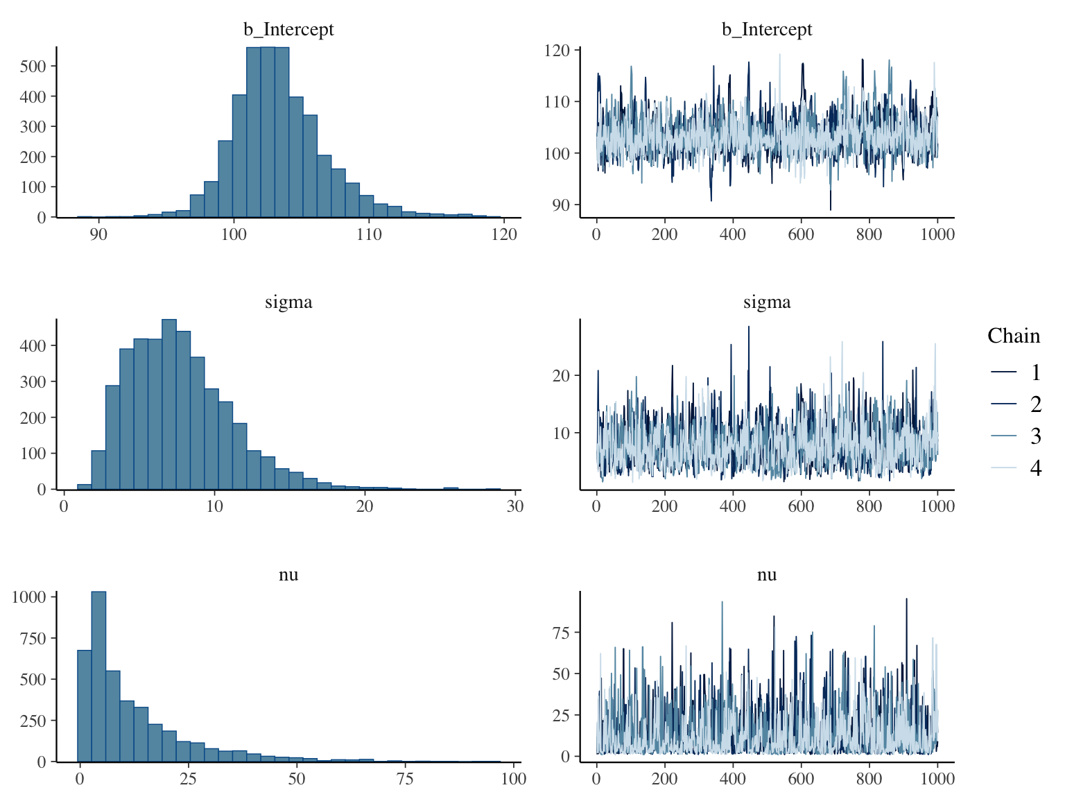
```{r bayesext2,h=6,w=8,cap='Posterior distributions for $\\mu, \\sigma, \\nu$ for a data model that is the $t$ distribution with $\\nu$ d.f. (left panels), and convergence diagnostics (right panels)',scap='Posterior distributions for $\\mu, \\sigma, \\nu$ for a $t_{\\nu}$ data model'}
#| label: fig-htset-bayesext2
prior_summary(g)
g
draws <- as.data.frame(g)
mu    <- draws$b_Intercept
P(mu > 110)
plot(g)
nu    <- draws$nu
snu   <- c(mean(nu), median(nu), pmode(nu))
ssd   <- c(sd(y), pmode(sigma), pmode(draws$sigma))
fm    <- function(x) paste(round(x, 2), collapse=', ')
```
* Posterior means discount the high outlier a bit and shows lower chance of $\mu > 110$
* The credible interval for $\mu$ is significantly smaller than the confidence interval due to allowance for heavy tails
* The posterior mean, median, and mode of $\nu$ (`r fm(snu)`) provide evidence that the data come from a distribution that is heavier tailed than the normal. Posterior $P(\nu > 20) =$ `r round(P(nu > 20), 2)` which is essentially the probability of approximate normality under a $t$ data model.
* The traditional SD estimate, posterior median SD assuming normal $Y$, and posterior median SD assuming $Y$ has a $t$-distribution are respectively `r fm(ssd)`. The ordinary SD is giving too much weight to the high outlier.
This latter analysis properly penalizes for not knowing normality in
$Y$ to hold (i.e., not knowing the true value of $\nu$).
#### Decoding the Effect of the Prior
* One can compute the effective number of observations added or subtracted by using, respectively, an optimistic or a skeptical prior
* This is particularly easy when the prior is normal, the data model is normal, and the data variance is known
* Let<br> $\mu_{0} =$ prior mean<br> $\sigma_{0} =$ prior standard
deviation<br> $\overline{Y} =$ sample mean of the response variable<br>
$\sigma =$ population SD of $Y$<br> $n =$ sample size for
$\overline{Y}$
* Then the posterior variance of $\mu$ is<br> $\sigma^{2}_{p} = \frac{1}{\frac{1}{\sigma^{2}_{0}} + \frac{1}{\frac{\sigma^{2}}{n}}}$
* The posterior mean is<br> $\mu_{p} = \frac{\sigma^{2}_{p}}{\sigma^{2}_{0}} \times \mu_{0} + \frac{\sigma^{2}_{p}}{\frac{\sigma^{2}}{n}} \times \overline{Y}$
* For a given $\overline{Y}$, sample size $n$ and posterior $P(\mu > 110)$, what sample size $m$ would yield the same posterior probability under a flat prior?
* For a flat prior $\sigma_{0} = \infty$ so the posterior variance of $\mu$ would be $\frac{\sigma^{2}}{n}$ and the posterior mean would be $\overline{Y}$
* Equating $P(\mu > 110)$ for the weakly informative prior at sample size $n$ to that from noninformative prior at a sample size $m$ is the same as setting $P(\mu < 110)$ to be equal
* The probability that a Gaussian random variable with mean $a$ and standard deviation $b$ is less than 110 is $\Phi(\frac{110-a}{b})$ where $\Phi$ is the standard normal cumulative distribution function
* Solve for $m$ for a variety of $n, \overline{Y}, \sigma$
```{r solvem}
calc <- function(n, m, ybar, sigma, mu0, sigma0, cutoff) {
  vpost1 <- 1 / ((1 / (sigma0^2)) + 1 / ((sigma^2) / n))
  mupost1 <- mu0 * vpost1 / (sigma0 ^ 2) + ybar * vpost1 / ((sigma ^ 2) / n)
  vpost2 <- (sigma ^ 2) / m
  (110 - mupost1) / sqrt(vpost1) - (110 - ybar) / sqrt(vpost2)
}

# For a given n, ybar, sigma solve for m to get equal post. prob.
m <- function(n, ybar, sigma, sigma0=50, cutoff=110)
  round(uniroot(calc, interval=c(n / 2, 2 * n), n=n, ybar=ybar, sigma=sigma,
          mu0=150, sigma0=sigma0, cutoff=cutoff)$root, 1)
# Make sure that m=n when prior variance is huge
m(8, 100, 10, sigma0=50000)
# From here on use the original prior standard deviation of 50
# Now compute m when n=8 using our original prior assuming sigma=10 ybar=105
m(8, 105, 10)
# What about for two other sigmas
m(8, 105, 5)
m(8, 105, 15)
# What about two other ybar
m(8, 80, 10)
m(8, 120, 10)
# What if n were larger
m(15, 105, 10)
m(30, 105, 10)
m(300, 105, 10)
m(3000, 105, 10)
```
* Typical effect of prior in this setting is like adding or dropping one observation
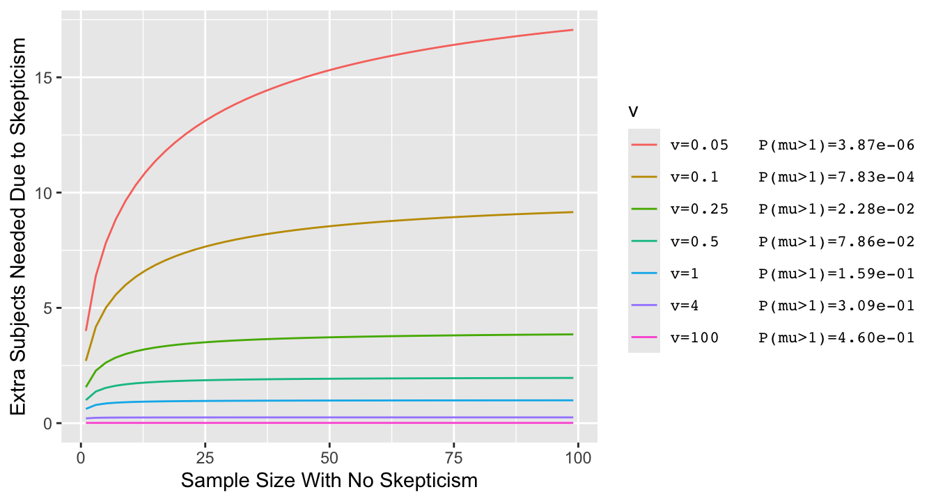
* Simpler example where $\overline{Y}$ is irrelevant: $\sigma=1, \mu_{0}=0$ and posterior probability of interest is $P(\mu > 0)$
* Vary the prior variance $\sigma^{2}_{0}$ and for each prior variance compute the prior probability that $\mu > 1$ (with prior centered at zero, lower variance $\rightarrow$ lower $P(\mu > 1)$)
```{r skepn,bty='l',cap="Effect of discounting by a skeptical prior with mean zero and variance v: the increase needed in the sample size in order to achieve the same posterior probability of $\\mu > 0$ as with the flat (non-informative) prior. Prior variance v=0.05 corresponds to a very skeptical prior, given almost no chance to a large $\\mu$ $(\\mu > 1)$.",scap="Effect of discounting by a skeptical prior"}
#| label: fig-htest-skepn
#| fig-height: 3.75
z    <- NULL
n    <- seq(1, 100, by=2)
vs   <- c(.05, .1, .25, .5, 1, 4, 100)
# Pad first part of text to 6 characterts so columns will line up
pad  <- function(x) substring(paste(x, '    '), 1, 6)
vlab <- paste0('v=', pad(vs), ' P(mu>1)=',
                format(1 - pnorm(sqrt(1 / vs)), digits=3, scientific=1))
names(vlab) <- as.character(vs)
for(v in vs)
  z <- rbind(z,
             data.frame(v, n, y = 0.5 * (n + sqrt(n^2 + 4 * n / v)) - n))
z$v <- factor(z$v, as.character(vs), vlab)
ggplot(z, aes(x=n, y=y, color=v)) + geom_line() +
  xlab('Sample Size With No Skepticism') +
  ylab('Extra Subjects Needed Due to Skepticism') +
  theme(legend.text = element_text(family='mono'))
```
* For typical priors the effect of skepticism is like dropping 3 observations, and this is not noticeable when $n > 20$^[See [here](http://hbiostat.org/bayes/bet/evidence.html#alternative-take-on-the-prior) for the derivation.]
* **Note**: For a specific problem one can just run the `brm` function again with a non-informative prior to help judge the effect of the informative prior
### Power and Sample Size
* Bayesian power is the probability of hitting a specified large posterior probability and is usually obtained by simulation
* Frequentist power, though often arbitrary (and inviting optimistic single point values for an effect to detect) is easier to
compute and will provide a decent approximation for Bayesian sample
size calculations when the main prior is weakly informative
* Frequentist power $\uparrow$ when
+ allow larger type I error ($\alpha$; trade-off between type I and II errors)
+ true $\mu$ is far from $\mu_{0}$
+ $\sigma \downarrow$
+ $n \uparrow$
* Power for 2-tailed test is a function of $\mu, \mu_{0}$ and $\sigma$ only through $|\mu - \mu_{0}| / \sigma$
* Sample size to achieve $\alpha=0.05$, power $=0.9$ is approximately
$$n = 10.51 [\frac{\sigma}{\mu-\mu_{0}}]^{2}$$
* Some power calculators are [here](https://statpages.info#Power)
* [PS program](https://cqsclinical.app.vumc.org/ps) by Dupont and Plummer (see also [G\*Power](https://www.psychologie.hhu.de/arbeitsgruppen/allgemeine-psychologie-und-arbeitspsychologie/gpower))
* Example: The mean forced expiratory volume (FEV) in a population of asthmatics is 2.5 liters per second and the population standard deviation is assumed to be 1. Determine the number of subjects needed if a new drug is expected to increase FEV to 3.0 liters per second ($\alpha = .05, \beta = 0.1$)
\begin{array}{c}
\mu=2.5, \mu_0=3, \sigma = 1 \\
n = 10.51 \left[\frac{1}{3-2.5}\right]^{2} = 42.04
\end{array}
* Rounding up, we need 43 subjects to have 0.9 power (42 subjects would have less than 0.9 power)
```{r powerone}
sigma <- 1
mu    <- 2.5
mu0   <- 3
n     <- 10.51 * (1 / (mu - mu0)) ^ 2
# General formula for approximate power of 1-sample t-test
# Approximate because it uses the normal distribution throughout,
# not the t distribution
alpha <- 0.05
power <- 0.9
delta <- mu - mu0
za    <- qnorm(1 - alpha / 2)
zb    <- qnorm(power)
n     <- ((za + zb) * sigma / delta) ^ 2
c(alpha=alpha, power=power, delta=delta, za=za, zb=zb, n=n)
```
A slightly more accurate estimate can be obtained using the $t$
distribution, requiring iterative calculations programmed in `R`
packages such as `pwr`.
```{r pwrpacktone}
# Make sure pwr package is installed
require(pwr)
pwr.t.test(d = delta / sigma, power = 0.9, sig.level = 0.05, type='one.sample')
```
### Confidence Interval
`r mrg(abd("6.6"))`
A 2-sided $1-\alpha$ confidence interval for $\mu$ under normality for $Y$ is
$$\bar{x} \pm t_{n-1,1-\alpha/2} \times \mathrm{se}$$
The $t$ constant is the $1-\alpha/2$ level critical value from the
$t$-distribution with $n-1$ degrees of freedom. For large $n$ it
equals 1.96 when $\alpha=0.05$.
An incorrect but common way to interpret this is that we are 0.95
confident that the
unknown $\mu$ lies in the above interval. The exact way to say it is
that if we were able to repeat the same experiment 1000 times and
compute a fresh confidence interval for $\mu$ from each sample, we
expect 950 of the samples to actually contain $\mu$. The confidence
level is about the procedure used to derive the interval, not about
any one interval. Difficulties in
providing exact but still useful interpretations of confidence intervals has driven
many people to Bayesian statistics.
The 2-sided $1-\alpha$ CL includes $\mu_{0}$ if and only if a test of $H_{0}:
\mu=\mu_{0}$ is not rejected at the $\alpha$ level in a 2-tailed test.
* If a 0.95 CL does not contain zero, we can reject $H_0: \mu = 0$ at the $\alpha = 0.05$ significance level
$1 - \alpha$ is called the _confidence level_ or _confidence coefficient_, but it is better to refer to _compatibility_
### Sample Size for a Given Precision
`r mrg(abd("14.7"))`
There are many reasons for preferring to run estimation studies
instead of hypothesis testing studies. A null hypothesis may be
irrelevant, and when there is adequate precision one can learn from a
study regardless of the magnitude of a $P$-value. A nearly universal
property of precision estimates is that, all other things being equal,
increasing the sample size by a factor of four improves the precision
by a factor of two.
* May want to estimate $\mu$ to within a margin of error of $\pm \delta$ with 0.95 confidence^[@adc97sam presents both frequentist and Bayesian methods and for precision emphasizes solving for $n$ such that the probability of being within $\epsilon$ of the true value is controlled, as opposed to using confidence interval widths explicitly.]
* "0.95 confident" that a confidence interval includes the true value of $\mu$
* If $\sigma$ were known but we still used the $t$ distribution in the formula for the interval, the confidence interval would be $\bar{x}\pm \delta$ where
$$\delta = \frac{t_{n-1,1-\alpha/2}\sigma}{\sqrt{n}}$$
* Solving for $n$ we get
$$n = \left[\frac{t_{n-1,1-\alpha/2} \sigma}{\delta}\right]^{2}$$
* If $n$ is large enough and $\alpha=0.05$, required $n=3.84[\frac{\sigma}{\delta}]^{2}$
* Example: if want to be able to nail down $\mu$ to within $\pm 1$mmHg when the patient to patient standard deviation in blood pressure is 10mmHg, $n = 384$
```{r precmean}
sigma <- 10
delta <- 1
3.84 * (sigma / delta) ^ 2
```
* Advantages of planning for precision rather than power^[See Borenstein M: _J Clin Epi_ 1994; 47:1277-1285.]
+ do not need to select a single effect to detect
+ many studies are powered to detect a miracle and nothing less; if a miracle doesn't happen, the study provides **no** information
+ planning on the basis of precision will allow the resulting study to be interpreted if the $P$-value is large, because the confidence interval will not be so wide as to include both clinically significant improvement and clinically significant worsening
## One Sample Method for a Probability
`r mrg(abd("7"))`
### Frequentist Methods
* Estimate a population probability $p$ with a sample estimate $\hat{p}$
* Data: $s$ "successes" out of $n$ trials
* Maximum likelihood estimate of $p$ is $\hat{p} = \frac{s}{n}$ (value of $p$ making the data most likely to have been observed) = Bayesian posterior mode under a flat prior
* Approximate 2-sided test of $H_{0}: p=p_{0}$ obtained by computing a $z$ statistic
* A $z$-test is a test assuming that the _statistic_ has a normal distribution; it is a $t$-test with infinite ($\infty$) d.f.
$$z = \frac{\hat{p} - p_{0}}{\sqrt{p_{0}(1-p_{0})/n}}$$
* The $z$-test follows the same general form as the $t$-test
$$z = \frac{\textrm{estimate - hypothesized value}}{\textrm{standard deviation of numerator}}$$
* Example: $n=10$ tosses of a coin, 8 heads; $H_{0}$: coin is fair ($p = p_{0}=\frac{1}{2}$)
$$z = \frac{.8 - .5}{\sqrt{(\frac{1}{2})(\frac{1}{2})/10}} = 1.897$$
* $P\textrm{-value} = 2 \times$ area under a normal curve to the right of $1.897 = 2 \times 0.0289 = 0.058$ (this is also the area under the normal curve to the right of $1.897$ + the area to the left of $-1.897$)
```{r zprop}
p  <- 0.8
p0 <- 0.5
n  <- 10
z  <- (p - p0) / sqrt(p0 * (1 - p0) / n)
c(z=z, Pvalue=2 * pnorm(-abs(z)))
```
* Approximate probability of getting 8 or more or 2 or fewer heads if the coin is fair is 0.058. **This is indirect evidence for fairness, is not the probability the null hypothesis is true, and invites the "absence of evidence is not evidence of absence" error.**
* Use exact methods if $p$ or $n$ is small
```{r exactprob}
# Pr(X >= 8) = 1 - Pr(X < 8) = 1 - Pr(X <= 7)
pbinom(2, 10, 0.5) + 1 - pbinom(7, 10, 0.5)
# Also compute as the probability of getting 0, 1, 2, 8, 9, 10 heads
sum(dbinom(c(0, 1, 2, 8, 9, 10), 10, 0.5))
```
* Confidence interval for $p$
+ [Wilson's method](https://en.wikipedia.org/wiki/Binomial_proportion_confidence_interval) without continuity correction is recommended
+ for 8 of 10 heads here is the Wilson interval in addition to the exact binomial and normal approximation. The Wilson interval is the most accurate of the three [@and23wal]
```{r wilson}
binconf(8, 10, method='all')
```
### Bayesian
* The single unknown probability $p$ for binary $Y$-case is a situation where there is a top choice for prior distributions
* Number of events follows a binomial distribution with parameters $p, n$
* The beta distribution is for a variable having a range of $[0, 1]$, has two parameters $\alpha, \beta$ for flexibility, and is _conjugate_ to the binomial distribution
+ The posterior distribution is simple: another beta distribution
* The mean of a beta-distributed variable is $\frac{\alpha}{\alpha + \beta}$ and its standard deviation is<br> $\sqrt{\frac{\alpha\beta}{\alpha+\beta+1}} / (\alpha + \beta)$
* Using a beta prior is equivalent to adding $\alpha$ successes and $\beta$ failures to the data
* Posterior distribution of $p$ is beta$(s + \alpha, n - s + \beta)$
* A uniform prior sets $\alpha = \beta = 1$
* In general an intuitive way to set the prior is to preset the mean then solve for the parameters that force $P(p > c) = a$ for given $c$ and $a$
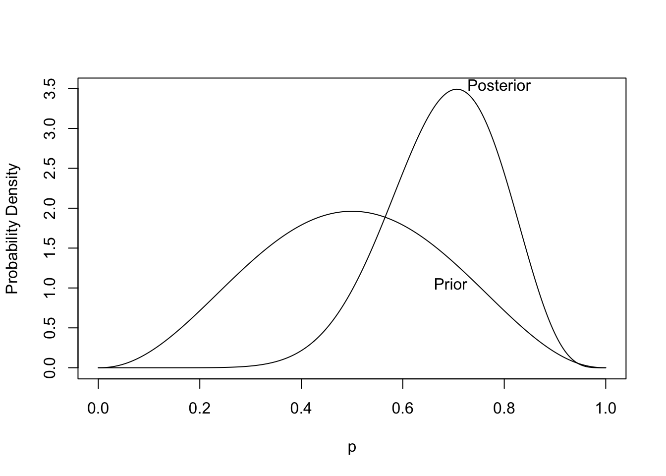
* For the 10 coin toss example let's set the prior mean of P$($heads$)=\frac{1}{2}$ and $P(p > 0.8) = 0.05$, i.e. only a 0.05 chance that the probability of heads exceeds 0.8. Here are $\alpha$ and $\beta$ satisfying these requirements:
```{r solveb}
# alpha/(alpha + beta) = 0.5 -> alpha=beta
alphas <- seq(0, 20, length=100000)
exceedanceProb <- 1 - pbeta(0.8, alphas, alphas)
alpha <- alphas[which.min(abs(exceedanceProb - 0.05))]
beta  <- alpha
alpha.post <- 8 + alpha
beta.post  <- 10 - 8 + beta
```
* The solution is $\alpha=\beta=`r round(alpha, 2)`$
* With the data $s=8$ out of $n=10$ the posterior distribution is beta (`r round(alpha.post, 2)`, `r round(beta.post, 2)`)
```{r plotbetapost,bty='l',cap='Prior and posterior distribution for the unknown probability of heads. The posterior is based on tossing 8 heads out of 10 tries.',scap='Prior and posterior distributions for unknown probability of heads'}
#| label: fig-htest-plotbetapost
p <- seq(0, 1, length=300)
prior <- dbeta(p, alpha, beta)
post  <- dbeta(p, alpha.post, beta.post)
curves <- list(Prior=list(x=p, y=prior),
               Posterior=list(x=p, y=post))
labcurve(curves, pl=TRUE, xlab='p', ylab='Probability Density')
```
* From the posterior distribution we can get the credible interval, the probability that the probability of heads exceeds $\frac{1}{2}$, and the probability that the probability of heads is within $\pm 0.05$ of fairness:
```{r betaprobs}
qbeta(c(.025, .975), alpha.post, beta.post)
1 - pbeta(0.5, alpha.post, beta.post)
pbeta(0.55, alpha.post, beta.post) - pbeta(0.45, alpha.post, beta.post)
```
* Unlike the frequentist analysis, these are direct measures that are easier to interpret
* Instead of just providing evidence against a straw-man assertion, Bayesian posterior probabilities measure evidence in favor (as well as against) all possible assertions
### Power and Sample Size
* Power $\uparrow$ as $n \uparrow$, $p$ departs from $p_{0}$, or $p_{0}$ departs from $\frac{1}{2}$
* $n \downarrow$ as required power $\downarrow$ or $p$ departs from $p_{0}$
### Sample Size for Given Precision{#sec-htest-p-n}
* Approximate 0.95 CL: $\hat{p} \pm 1.96 \sqrt{\hat{p}(1-\hat{p})/n}$
* Assuming $p$ is between 0.3 and 0.8, it would not be far off to use the worst case standard error $\sqrt{1/(4n)}$ when planning
* $n$ to achieve a margin of error $\delta$ in estimating $p$:
$$n = \frac{1}{4}\left[\frac{1.96}{\delta}\right]^{2} = \frac{0.96}{\delta^{2}}$$
* Example: $\delta=.1 \rightarrow n=96$ to achieve a margin of error of $\pm 0.1$ with 0.95 confidence
```{r nmoep}
nprec <- function(delta) round(0.25 * (qnorm(0.975) / delta) ^ 2)
nprec(0.1)
```
To achieve a margin of error of $\pm 0.05$ even in the worst case where
$p=0.5$ one needs $n=`r nprec(0.05)`$.
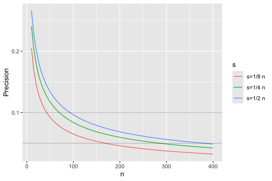
For Bayesian precision calculations we can solve $n$ that achieves a
given width of, say, a 0.95 credible interval:
* Use a flat beta prior, i.e., with $\alpha=\beta=1$
* Posterior distribution for $p$ is $\textrm{beta}(s + 1, n - s + 1)$
* Compute CI half-widths for varying $n$ for selected values of $s$
```{r pprecb,bty='l',h=4,w=6,cap='Half-widths of 0.95 credible intervals for $p$ using a flat prior'}
#| label: fig-htest-pprecb
n <- seq(10, 400, by=5)
k <- c(1/8, 1/4, 1/2)
ck <- paste0('s=', c('1/8', '1/4', '1/2'), ' n')
r <- NULL
for(i in 1 : 3) {
   ciu <- qbeta(0.975, k[i] * n + 1, n - k[i] * n + 1)
   cil <- qbeta(0.025, k[i] * n + 1, n - k[i] * n + 1)
     r   <- rbind(r, data.frame(n, y=(ciu - cil) / 2, s=ck[i]))
}
r$s <- factor(r$s, ck)
ggplot(r, aes(x=n, y, col=s)) + geom_line() +
  ylab('Precision') +
  geom_abline(slope=0, intercept=c(0.05, 0.1), alpha=I(0.25))
```
* As with confidence intervals, precision is worst when $\frac{1}{2}$ of observations are successes, so often best to plan on worst case
* Same sample size needed as with frequentist (since prior is flat)
* Easy to modify for other priors
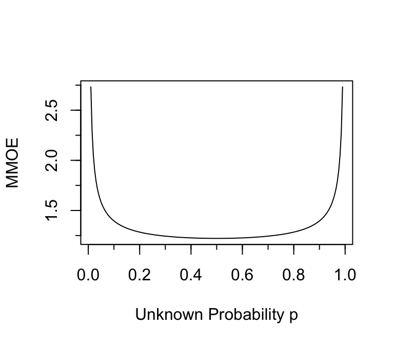
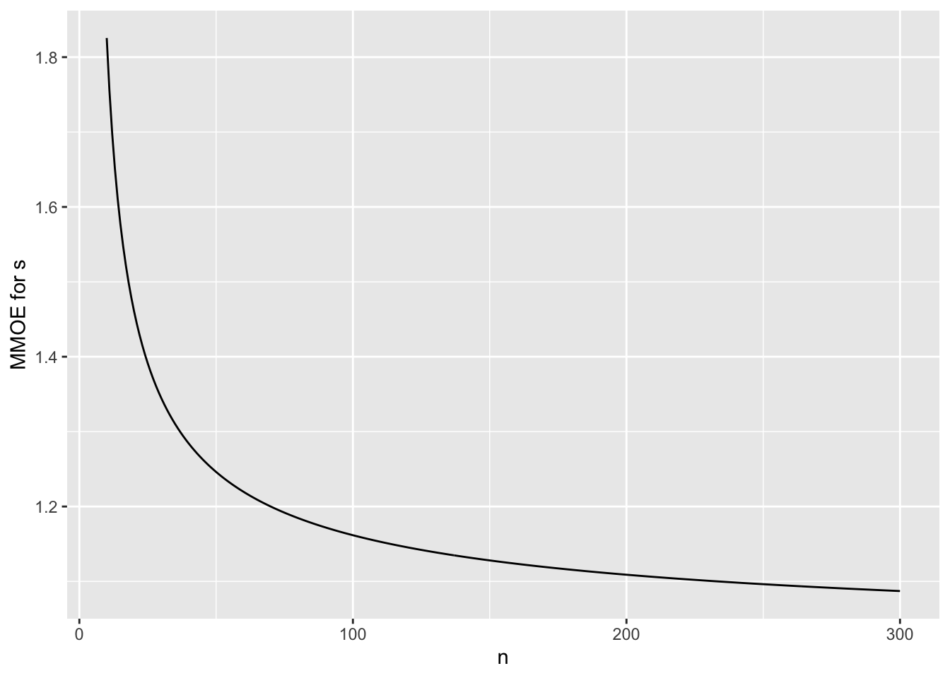
To put this in the context of relative errors, suppose that one wants
to estimate the odds that an event will occur, to within a certain
multiplicative margin of error (MMOE) with 0.95 confidence using
frequentist methods. What is
the MMOE as a function of the unknown $p$ when $n=384$? The standard
error of the log odds is approximately $\sqrt{\frac{1}{n p (1 - p)}}$,
and the half-width of a 0.95 confidence interval for the log odds is
approximately 1.96 times that. Fix $n=384$ and vary $p$ to get the
MMOE that is associated with the same sample size as a universal
absolute margin of error of 0.05.
```{r moeor,w=4,h=3.5,cap='Multiplicative margin of error in estimating odds when $n=384$ and the margin of error in estimating the absolute probability is $\\leq 0.05$.'}
#| label: fig-htest-moeor
p <- seq(0.01, 0.99, length=200)
mmoe <- exp(1.96 / sqrt(384 * p * (1 - p)))
plot(p, mmoe, type='l', xlab='Unknown Probability p', ylab='MMOE')
minor.tick()
```
## Paired Data and One-Sample Tests
`r mrg(abd("11"))`
* To investigate the relationship between smoking and bone mineral density, Rosner presented a paired analysis in which each person had a nearly perfect control which was his or her twin
* Data were normalized by dividing differences by the mean density in the twin pair (need to check if this normalization worked)
* **Note**: It is almost never appropriate to compute mean percent change (a 100\% increase is balanced by a 50\% decrease) but we plunge ahead anyway
* Computed density in heavier smoking twin minus density in lighter smoking one
* Mean difference was $-5\%$ with se=$2.0\%$ on $n=41$
* The $t$ statistic we've been using works here, once within-pair differences are formed
* $H_{0}:$ mean difference between twins is zero ($\mu_{0} = 0$)
\begin{array}{c}
t_{40} = \frac{\bar{x} - \mu_{0}}{se} = -2.5 \\
P = 0.0166
\end{array}
```{r ptwins}
xbar  <- -5
se    <- 2
n     <- 41
mu0   <- 0
tstat <- (xbar - mu0) /se
pval  <- 2 * (1 - pt(abs(tstat), n - 1))
c(tstat=tstat, Pvalue=pval)
```
## Two Sample Test for Means
`r mrg(abd("12"), bmovie(6), ddisc(6))`
* Two groups of different patients (unpaired data)
* Much more common than one-sample tests
* As before we are dealing for now with parametric tests assuming the raw data arise from a normal distribution
* We assume for now that the two groups have the same spread or variability in the distributions of responses^[Rosner covers the unequal variance case very well. As nonparametric tests have advantages for comparing two groups and are less sensitive to the equal spread assumption, we will not cover the unequal variance case here.]
### Frequentist $t$-Test
* Test whether population 1 has the same mean as population 2
* Example: pop. 1=all patients with a certain disease if given the new drug, pop. 2=standard drug
* $H_{0}: \mu_{1}=\mu_{2}$ (this can be generalized to test $\mu_{1}=\mu_{2}+\delta$, i.e., $\mu_{1}-\mu_{2}=\delta$). The _quantity of interest_ or _QOI_ is $\mu_{1}-\mu_{2}$
* 2 samples, of sizes $n_{1}$ and $n_{2}$ from two populations
* Two-sample (unpaired) $t$-test assuming normality and equal variances---recall that if we are testing against an $H_0$ of
**no effect**, the form of the $t$ test is
$$t = \frac{\mathrm{point~estimate~of~QOI}}{\mathrm{se~of~numerator}}$$
* Point estimate QOI is $\bar{x}_{1} - \bar{x}_{2}$
* As with 1-sample $t$-test the difference in the numerator is judged with respect to the precision in the denominator (combination of sample size and subject-to-subject variability); like a signal:noise ratio
* Variance of the sum or difference of two independent means is the sum of the variance of the individual means
* This is $\frac{\sigma^{2}}{n_{1}} + \frac{\sigma^{2}}{n_{2}} = \sigma^{2}[\frac{1}{n_{1}} + \frac{1}{n_{2}}]$
* Need to estimate the single $\sigma^{2}$ from the two samples
* We use a weighted average of the two sample variances:
$$s^{2} = \frac{(n_{1}-1)s^{2}_{1} + (n_{2}-1)s^{2}_{2}}{n_{1}+n_{2}-2}$$
* True standard error of the difference in sample means: $\sigma \sqrt{\frac{1}{n_{1}} + \frac{1}{n_{2}}}$
* Estimate: $s \sqrt{\frac{1}{n_{1}} + \frac{1}{n_{2}}}$, so
$$t = \frac{\bar{x}_{1} - \bar{x}_{2}}{s \sqrt{\frac{1}{n_{1}} + \frac{1}{n_{2}}}}$$
* d.f. is the sum of the individual d.f., $n_{1}+n_{2}-2$, where the $-2$ is from our having to estimate the center of two distributions
* If $H_{0}$ is true $t$ has the $t_{n_{1}+n_{2}-2}$ distribution
* To get a 2-tailed $P$-value we compute the probability that a value from such a distribution is farther out in the tails of the distribution than the observed $t$ value is (we ignore the sign of $t$ for a 2-tailed test)
* Example: $n_{1}=8, n_{2}=21, s_{1}=15.34, s_{2}=18.23, \bar{x}_{1}=132.86, \bar{x}_{2}=127.44$
\begin{array}{ccc}
s^{2} &=& \frac{7(15.34)^{2}+20(18.23)^{2}}{7+20} = 307.18 \\
s &=& \sqrt{307.18} = 17.527 \\
se &=& 17.527 \sqrt{\frac{1}{8}+\frac{1}{21}} = 7.282 \\
t &=& \frac{5.42}{7.282} = 0.74
\end{array}
on 27 d.f.
* $P = 0.463$ (see `R` code below)
* Chance of getting a difference in means as larger or larger than 5.42 if the two populations really have the same means is 0.463
* $\rightarrow$ little evidence for concluding the population means are different
```{r ptwot}
n1    <- 8;         n2 <- 21
xbar1 <- 132.86; xbar2 <- 127.44
s1    <- 15.34;     s2 <- 18.23
s     <- sqrt(((n1 - 1) * s1 ^ 2 + (n2 - 1) * s2 ^ 2) / (n1 + n2 - 2))
se    <- s * sqrt(1 / n1 + 1 / n2)
tstat <- (xbar1 - xbar2) / se
pval  <- 2 * (pt(- abs(tstat), n1 + n2 - 2))
c(s=s, se=se, tstat=tstat, Pvalue=pval)
```
### Confidence Interval
Assuming equal variances
$$\bar{x}_{1}-\bar{x}_{2} \pm t_{n_{1}+n_{2}-2,1-\alpha/2} \times s \times \sqrt{\frac{1}{n_{1}} + \frac{1}{n_{2}}}$$
is a $1-\alpha$ CL for $\mu_{1}-\mu_{2}$, where $s$ is the pooled
estimate of $\sigma$, i.e., $s \sqrt{\ldots}$ is the estimate of the
standard error of $\bar{x}_{1}-\bar{x}_{2}$
### Probability Index {#sec-htest-pi}
The _probability index_ or _concordance probability_ $c$ for a two-group comparison is a useful unitless index of an effect. If $Y_1$ and $Y_2$ represent random variables from groups 1 and 2 respectively, $c = \Pr(Y_{2} > Y_{1}) + \frac{1}{2} \Pr(Y_{2} = Y_{1})$ which is the probability that a randomly chosen subject from group 2 has a response exceeding that of a randomly chosen subject from group 1, plus $\frac{1}{2}$ the probability they are tied. $c$ can be estimated nonparametrically by the fraction of all possible pairs of subjects (one from group 1, one from group 2) with $Y_{2} > Y_{1}$ plus $\frac{1}{2}$ the fraction of ties. This is related to Somers' $D_{yx}$ rank correlation coefficient by $D_{yx} = 2 \times (c - \frac{1}{2})$.
When $Y_i$ comes from a normal distribution with mean $\mu_i$ and variance $\sigma^2$ (equal variance case), the probability of a tie is zero, the SD of $Y_{2}-Y_{1}$ is $\sqrt{2}\sigma$, and we have the following after letting the difference in population means $\mu_{2} - \mu_{1}$ be denoted by $\delta$.
\begin{array}{lcl}
c = \Pr(Y_{2} > Y_{1}) &=& \Pr(Y_{2} - Y_{1} > 0) \\
&=& \Pr(Y_{2} - Y_{1} - \delta > - \delta)\\
&=& \Pr(\frac{Y_{2} - Y_{1} - \delta}{\sqrt{2}\sigma} > - \frac{\delta}{\sqrt{2}\sigma}) \\
&=& 1 - \Phi(- \frac{\delta}{\sqrt{2}\sigma}) = \Phi(\frac{\delta}{\sqrt{2}\sigma})
\end{array}
where $\Phi(x)$ is the standard normal cumultive distribution function.
When the variances are unequal, the variance of $Y_{2} - Y_{1}$ is $\sigma_{2}^{2} + \sigma_{1}^{2}$ so the SD is $\sqrt{\sigma_{2}^{2} + \sigma_{1}^{2}} = \omega = \sigma_{1}\sqrt{1 + r}$ where $r$ is the variance ratio $\frac{\sigma_{2}^{2}}{\sigma_{1}^{2}}$. The probability index $c$ is $\Phi(\frac{\delta}{\omega})$. $r$ doesn't matter if there is no group mean difference ($\delta=0$). But when $\delta \neq 0$ the probability index depends on the variance ratio.
### Bayesian $t$-Test
* As with one-sample Bayesian $t$-test we relax the normality assumption by using a $t$ distribution for the raw data (more robust analysis)
* A linear model for the two-sample $t$ test is<br> $Y = \mu_{0} + \delta[\textrm{group B}] + \epsilon$<br> where $\mu_{0}$ (the intercept) is the unknown group A mean, $\delta$ is the B-A difference in means, and $\epsilon$ is the irreducible residual (assuming we have no covariates to adjust for)
* Assume:
+ $\epsilon$ has a $t$-distribution with $\nu$ d.f.
+ $\nu$ has a prior that allows the data distribution to be anywhere from heavy-tailed to normal
+ $\mu_{0}$ has a fairly wide prior distribution (no prior knowledge may be encoded by using a flat prior)
+ $\delta$ has either a prior that is informed by prior reliable research or biological knowledge, or has a skeptical prior
+ residual variance $\sigma^2$ is allowed to be different for groups A and B, with a normal prior on the log of the variance ratio that favors equal variance but allows the ratio to be different from 1 (but not arbitrarily different)
Note: by specifying independent priors for $\mu_{0}$ and $\delta$ we
+ induce correlations in priors for the two means
+ assume we know more about $\delta$ than about the individual true per-group means
To specify the SD for the prior for the log variance ratio:
* Let $r$ be unknown ratio of variances
* Assume $P(r > 1.5) = P(r < \frac{1}{1.5}) = \gamma$
* The required SD is $\frac{\log{1.5}}{-\Phi^{-1}(\gamma)}$
* For $\gamma=0.15$ the required SD is:
```{r priorsigma}
log(1.5) / -qnorm(0.15)
```
We are assuming a mean of zero for $\log(r)$ so we favor $r=1$ and give equal chances to ratios smaller or larger than 1.
### Power and Sample Size
* Consider the frequentist model
* Power increases when
+ $\Delta = |\mu_{1}-\mu_{2}| \uparrow$
+ $n_{1} \uparrow$ or $n_{2} \uparrow$
+ $n_{1}$ and $n_{2}$ are close
+ $\sigma \downarrow$
+ $\alpha \uparrow$
* Power depends on $n_{1}, n_{2}, \mu_{1}, \mu_{2}, \sigma$ approximately through
$$\frac{\Delta}{\sigma \sqrt{\frac{1}{n_{1}}+\frac{1}{n_{2}}}}$$
* Note that when computing power using a program that asks for $\mu_{1}$ and $\mu_{2}$ you can just enter 0 for $\mu_{1}$ and enter $\Delta$ for $\mu_{2}$, as only the difference matters
* Often we estimate $\sigma$ from pilot data, and to be honest we should make adjustments for having to estimate $\sigma$ although we usually run out of gas at this point (Bayes would help)
* Use the `R` `pwr` package, or the power calculator at [statpages.org](statpages.org#Power) or PS
* Example: <br> Get a pooled estimate of $\sigma$ using $s$ above (`r round(s, 3)`) <br> Use $\Delta=5, n_{1}=n_{2}=100, \alpha=0.05$
<!-- $\sqrt{\frac{15.34^{2}+18.23^{2}}{2}} =--->
<!-- 16.847$ when--->
```{r tuneqpow}
delta <- 5
require(pwr)
pwr.t2n.test(n1=100, n2=100, d=delta / s, sig.level = 0.05)
```
* Sample size depends on $k = \frac{n_{2}}{n_{1}}$, $\Delta$, power, and $\alpha$
* Sample size $\downarrow$ when
+ $\Delta \uparrow$
+ $k \rightarrow 1.0$
+ $\sigma \downarrow$
+ $\alpha \uparrow$
+ required power $\downarrow$
* An approximate formula for required sample sizes to achieve power $=0.9$ with $\alpha=0.05$ is
\begin{array}{ccc}
n_{1} &=& \frac{10.51 \sigma^{2} (1+\frac{1}{k})}{\Delta^{2}} \\
n_{2} &=& \frac{10.51 \sigma^{2} (1+k)}{\Delta^{2}}
\end{array}
<!-- * Example using web page: <br>--->
<!-- Does not allow unequal $n_1$ and $n_2$; use power=0.8, $\alpha=0.05,--->
<!-- \mu_{1}=132.86, \mu_{2}=127.44, \sigma=16.847$--->
<!-- * Result is 153 in each group (total=306) vs. Rosner's--->
<!-- $n_{1}=108, n_{2}=216$, total=324. The price of having unequal--->
<!-- sample sizes was 18 extra patients.--->
* Exact calculations assuming normality
```{r ssizet}
pwr.t.test(d = delta / s, sig.level = 0.05, power = 0.8)
```
* If used same total sample size of 388 but did a 2:1 randomization ratio to get 129 in one group and 259 in the other, the power is less
```{r powtuneqn}
pwr.t2n.test(n1 = 129, n2 = 259, d = delta / s, sig.level = 0.05)
```
What is the difference in means that would yield a 2-sided $P$-value
of exactly 0.05 for a two-sample $t$-test with normality and equal
variances when the sample sizes are both equal to $\frac{n}{2}$? We
solve for $\hat{\Delta} = \bar{x}_{1} - \bar{x}_{2}$ such
that $t_{n-2,1-\alpha/2} = \frac{\hat{\Delta}}{2s/\sqrt{n}}$, giving
$$\hat{\Delta} = \frac{2 \times t_{n-2,1-\alpha/2} \times s}{\sqrt{n}}$$
For total sample sizes of 10, 50, and 100, the "magic" values of the
observed difference are the following multiples of the observed
standard deviation $s$:
```{r deltathresh}
n <- c(10, 50, 100)
tcrit <- qt(0.975, n-2)
2 * tcrit / sqrt(n)
```
Note that these thresholds are independent of the power and the effect
size used in the power calculation.
### Sample Size for a Given Precision{#sec-htest-t2-moe}
To design a study that will nail down the estimate of $\mu_{1}-\mu_{2}$
to within $\pm \delta$ with $1-\alpha$ confidence when $n_{1}=n_{2}=n$, and
when $n$ is large enough so that the critical value
$t_{2n-2,1-\alpha/2}$ may be approximated by the critical value from
the normal distribution, say $z$ ($z=1.96$ when $\alpha=0.05$):
$$n = 2\left[\frac{z \sigma}{\delta}\right]^{2}$$
When $\alpha=0.05$, $n = 7.68 [\frac{\sigma}{\delta}]^{2}$
### Equating Margin of Error to Detectable Difference
Suppose that a two-arm study is designed to detect a difference $\Delta$ in two
means with power 0.9 at the $\alpha=0.05$ level. For large enough
sample sizes, the margin of error for estimating the true difference
in means for that study will be
$\delta = \Delta\sqrt{\frac{7.68}{21.02}} = 0.604\Delta$.
### Checking Assumptions of the $t$-test
* Comprehensive assessment of all assumptions except independence of observations:
+ Compute the two empirical cumulative distribution functions
+ Transform each using the inverse normal $z$ transformation
+ See of both curves are linear (checks normality assumption) and parallel (equal variance assumption)^[There are formal tests of normality but in smaller samples these have insufficient power to detect important non-normality.]
* Box plot (one box for each of 2 groups): look for equal spread
(IQR)
* Informally compare $s_{1}$ and $s_{2}$^[Rosner 8.6 shows how to make formal comparisons, but beware that the variance ratio test depends on normality, and it may not have sufficient power to detect important differences in variances.]
* With the Bayesian $t$-test the only important assumption to check is symmetry of the data distribution^[Since we are allowing for heavier tails than the Gaussian distribution by using a $t$ distribution for the raw data]
## Comprehensive Example: Two sample $t$-test
### Study Description
* Assess the effect of caffeine (vs. placebo) on muscle
metabolism, measured by the respiratory exchange ratio (RER; ratio
of CO$_{2}$ produced to O$_{2}$ consumed) [Dataset was from a study done by the University of Bristol UWE; web site no longer available]{.aside}
* Treatment was randomized to 18 subjects; parallel group RCT
* Goal: study effect of caffeine on RER
* Must take log of RER to have a symmetric measure
+ $\mu_0$ = mean log RER for placebo
+ $\mu_1$ = mean log RER for caffeine
+ Fold-change effect: $\exp(\mu_1 - \mu_0)$
+ Estimate $\mu_{1} - \mu_{0}$
+ $H_0: \mu_0 = \mu_1$
+ $H_1: \mu_0 \neq \mu_1$
* Note: a good statistician will take such ratios with a grain of salt; need to verify that the meaning of the ratio is independent of O$_{2}$
### Power and Sample Size
* Suppose that a pilot study or previous published research
estimated $\sigma = 0.1$ for log RER
* Effect size $\Delta$ is on the log RER scale
* Anti-log to get effect in terms of fold change
* Determine the number of subjects needed (in each group) for several value of effect size $\Delta$ ($\Delta = |\mu_1 - \mu_0|$) in order to have 0.9 power with $\alpha = 0.05$
```{r samsizerer}
require(pwr)
s <- 0.1
fc <- c(1.1, 1.15, 1.2, 1.25, 1.5)
n <- integer(length(fc))
i <- 0
for(foldchange in fc) {
  i <- i + 1
  n[i] <- ceiling(pwr.t.test(d=log(foldchange) / s, power=0.9)$n)
}
data.frame('Fold Change'=fc, Delta=round(log(fc), 3), 'N per group'=n,
           check.names=FALSE)
```
* If caffeine modifies RER by a factor of 1.15, by enrolling 12 subjects in each group we will have 0.9 power to detect an effect
* For $n=12$ per group the margin of error for estimating $\Delta$ at the 0.95 level is given below<br>
See @sec-htest-t2-moe
* This is anti-logged to obtain the multiplicative margin of error for estimating the caffeine:placebo ratio of RERs
```{r rmmoe}
z <- qnorm(0.975); n <- 12
# This is approximate; use z <- qt(0.975, 12+12-2) for accuracy
moe <- z * s * sqrt(2 / n)
mmoe <- exp(moe)
c('Margin of Error'=moe, 'Multiplicative Margin of Error'=mmoe)
```
### Collected Data
```{r rerdata}
tx <- factor(c(rep('placebo', 9), rep('caffeine', 9)), c('placebo', 'caffeine'))
rer <- c(105, 119, 100, 97, 96, 101, 94, 95, 98,
         96, 99, 94, 89, 96, 93, 88, 105, 88) / 100
d <- data.frame(subject=1:18, tx, rer, logrer=log(rer))
print(d, digits=3, row.names=FALSE)
```
```{r reraa,w=5,h=3,cap='Data for two-sample RCT for effect of caffeine on respiratory exchange ratio. Diamonds depict medians.',scap='Two-sample parallel group RCT'}
#| label: fig-htest-reraa
require(ggplot2)
ggplot(d, aes(x=tx, y=rer, group=tx)) +
  geom_boxplot(col='lightyellow1', alpha=.3, width=.3) +
  geom_dotplot(binaxis='y', stackdir='center', position='dodge') +
  stat_summary(fun.y=median, geom="point", col='red', shape=5, size=3) +
  xlab('') + ylab('RER') + coord_flip()
```
### Frequentist $t$-Test
To demonstrate difficulties in checking model assumptions with small $n$, consider the comprehensive approach by checking for linearity and parallelism (if equal variance assumption is used) of $z$-transformed empirical cumulative distributions.
```{r rerpass, w=5, h=3.75, bty='l', scap='Stratified ECDFs for checking $t$-test assumptions', cap='Stratified empirical cumulative distribution functions by treatment for checking all assumptions of the two-sample $t$-test. ECDFs are inverse normal transformed.'}
#| label: fig-htest-rerpass
Ecdf(~ log(rer), groups=tx, fun=qnorm, data=d,
     xlab='log(RER)', ylab='Inverse Normal ECDF')
```
It is more accepted in practice to now use the form of the $t$-test
that does not assume equal variances in the two independent groups.
The unequal-variance $t$-test is used here. Note that to compute a
decent approximation to the $P$-value requires the use of a "trick"
d.f. when looking up against a $t$ distribution.
```{r }
ttest <- t.test(log(rer) ~ tx, data=d)
# Note that for the CI t.test is using caffeine as the reference group
ttest
```
* Interpretation
+ Subjects given caffeine have on average a log RER that is 0.064
lower (0.95 CI: [-0.13, 0.002]) than individuals given placebo
+ By anti-logging these 3 numbers we get the fold change scale:
- Median^[If the log ratio has a normal distribution, the log ratio has the same mean as the median and its median anti-logged value is the anti-log of the mean (=median) log difference. The mean on the anti-logged scale is a more complex function that involves SD of log RER.] fold change is 0.94
- 0.95 CI for caffeine:placebo fold change: $[0.878, 1.002]$
### Bayesian $t$-Test
The `R` `brms` package makes it easy to specify an unequal variance
model, because it allows one to specify a separate model for the log
of the standard deviation. $\log(\sigma)$ can even depend on
continuous covariates!^[Thanks to Nathan James of the Vanderbilt Department of Biostatistics for providing `R` code for this section, and for providing the explanation for the output of the `prior_summary` function.] `brms` models standard deviation parameters on the log scale. As before, analysis is on the
log(RER) scale.
```{r bayesfit2}
require(brms)
# set priors

# flat (non-informative) prior for intercept
pr0 <- set_prior("", class="Intercept")

# normal(0,3) prior for difference in log ratios
pr1 <- set_prior("normal(0,0.25)", class="b", coef="txcaffeine")

# normal(0,0.3912) for log SD ratio
pr2 <- set_prior("normal(0,0.3912)", class="b", coef="txcaffeine",
                 dpar="sigma")

# fit model for two groups assuming Y follows a t distribution so less
# sensitive to outliers
# Each group has different mean and SD but same df
# The prior for the log SD for the reference group is scale t with 3 d.f.
# Prior for nu is gamma(2, 0.1)
# The bf function is used to create a compound R model formula, here
# for the mean model and the log sigma model

g <- function()
       brm(bf(log(rer) ~ tx, sigma ~ tx), data=d, family=student,
           prior=c(pr0,pr1,pr2), seed=1203)
f <- runifChanged(g, d, pr0, pr1, pr2)
```
There are 5 parameters in this model (2 for the regression on student-$t$ mean, 2 for the regression on student-$t$ scale ($\sigma$), and 1 for student-$t$ d.f. $\nu$). The output from `prior_summary()` shows all the parameters _and_ parameter classes that can be assigned. Lines 1 \& 3 in the output below are the `classes` of all non-intercept regression coefficients for the student-$t$ mean and student-$t$ scale, respectively. When there are multiple coefficients it is often convenient to specify a prior for all parameters in a class rather than for each individual parameter. For example, in a model with 10 covariates using `set_prior("normal(0,1)", class="b")` would give each of the 10 corresponding coefficient parameters a standard normal prior. For our model the class priors are superseded by the individual parameter priors.
```{r bayesfit2b, w=7.5, h=6}
# Show priors in effect
prior_summary(f)
# model summary
# Note: sigma is on log scale, use exp(sigma) to get to natural scale
# Intercept is mean for placebo
# sigma_Intercept is log(sd) for placebo
# txcaffeine is change in mean for caffeine compared to placebo
# sigma_txcaffeine is change in log(sd) for caffeine compared to placebo
f
# plot kernel density est and trace plots for posterior parameters
plot(f)
```
```{r bayesfit2c}
# posterior predictive check
pp_check(f)
```
```{r bayesfit2d}
# conditional effects
plot(conditional_effects(f), points = TRUE)
```
```{r bayesfit2e,mfrow=c(2,2),w=7,h=6}
# posterior parameter samples
p <- as.data.frame(f)
meanplacebo <- p[, 'b_Intercept']
delta       <- p[, 'b_txcaffeine']
sdplacebo   <- exp(p[, 'b_sigma_Intercept'])
sdratio     <- exp(p[, 'b_sigma_txcaffeine'])
nu          <- p[, 'nu']

# histogram of posterior distribution of difference in mean log RER
hist(delta, nclass=50, main='')
# Posterior density for caffeine:placebo fold change in RER
plot(density(exp(delta)), xlab='Fold Change in RER', main='')
abline(v=1, col=gray(0.85))
# Posterior density of SD ratio
plot(density(sdratio), main='', xlab='SD Ratio')
abline(v=1, col=gray(0.85))
# Posterior prob that difference in means < 0
# Recall that the P operator was defined previously
# (based on mean of logical or 0/1 values = proportion positive =
#  posterior probability to within simulation error
# This is the same as P(fold change < 1)
P(delta < 0)
P(exp(delta) < 1)
# Prob that caffeine results in a physiologically noticeable response
P(exp(delta) < 0.95)
# Prob that caffeine and placebo have similar response
P(exp(delta) > 0.975 & exp(delta) < 1/0.975)
# Compute posterior probability of approximate normality
P(nu > 20)
```
Note that the
2-tailed $P$-value of 0.057 may tempt bright-line threshold advocates
to conclude nothing more than insufficient evidence to reject the
assumption that caffeine does not modify RER (or worse yet to just declare
an "insignificant" result or even worse that caffeine does not modify
RER). The Bayesian result shows that under a fairly skeptical prior
for log RER one would do well to play the odds in betting on caffeine
having an effect.
There is little evidence to support an assumption of normality of log
RER within a treatment group.
Now compare other results results with the frequentist analysis.
```{r bayesfit2g}
means <- with(d, tapply(logrer, tx, mean))
sds   <- with(d, tapply(logrer, tx, sd))
a <- c(means[1],    pmode(meanplacebo), mean(meanplacebo), median(meanplacebo))
b <- c(sds[1],      pmode(sdplacebo),   mean(sdplacebo),   median(sdplacebo))
w <- c(diff(means), pmode(delta),     mean(delta),     median(delta))
z <- c(sds[2] / sds[1], pmode(sdratio), mean(sdratio), median(sdratio))
x <- rbind(a, b, w, z)
colnames(x) <- c('Sample', 'Posterior Mode', 'Posterior Mean',
                 'Posterior Median')
rownames(x) <- c('Placebo mean', 'Placebo SD', 'Caffeine - Placebo Mean',
                 'Caffeine / Placebo SD')
round(x, 2)
# 0.95 credible interval for delta
quantile(delta, c(0.025, .975))
# 0.95 confidence interval for delta
rev(- ttest$conf.int)   # negate since t.test used different reference
```
For an excellent tutorial on the use of `brms` for a two-sample $t$-test see [bit.ly/brms-t](https://vuorre.netlify.com/post/2017/01/02/how-to-compare-two-groups-with-robust-bayesian-estimation-using-r-stan-and-brms) by Matti Vuorre
## The Problem with Hypothesis Tests and $P$-values Revisited
### Hypothesis Testing
* Existence of ESP is a hypothesis
* Assessing effects of drugs, procedures, devices involves
estimation
* Many studies powered to detect huge effect
* If effect is not huge, no information from study
### $P$-Values
`r mrg(abd("6.2"))`
* Only provide evidence against a _null_ hypothesis,
**never** evidence for something
* Probability of a statistic _more_ impressive as yours **\Large if** $H_0$ true
* Not a probability of an effect or difference (same problem with
sensitivity and specificity)
* **No** conclusion possible from large $P$-values
* Cannot conclude clinical relevance from small $P$
* Adjustment of $P$-values for multiple tests is controversial and
there is insufficient consensus on how to choose an adjustment
method
* Declaring a result as "significant" or "non-significant" is completely arbitrary and has come to mean almost nothing
+ They rely on completely arbitrary $P$-value cutoffs such as 0.05
+ American Statistical Association is on record recommending not using any cutoff or words like _significant_: [bit.ly/asa-p](https://amstat.tandfonline.com/doi/full/10.1080/00031305.2016.1154108) [bit.ly/asa-p2](https://www.tandfonline.com/doi/full/10.1080/00031305.2019.1583913)
### How Not to Present Results
`r mrg(abd("6.2"))`
* $P=0.02$ --- let's put this into clinical practice ignoring the
drug's cost or clinical effectiveness
* $P=0.4$ --- this drug does not kill people
* $P=0.2$ but there is a trend in favor of our blockbuster drug
* The observed difference was 6mmHg and we rejected $H_0$ so the
true effect is 6mmHg.
* The proportion of patients having adverse events was 0.01 and
0.03; the study wasn't powered to detect adverse event differences
so we present no statistical analysis
* The reduction in blood pressure was 6mmHg with 0.95 C.L. of
[1mmHg, 11mmHg]; the drug is just as likely to only reduce blood
pressure by 1mmHg as it is by 6mmHg.
* The serum pH for the 15 dogs was $7.3 \pm 0.1$ (mean $\pm$ SE instead of SD or IQR)
### How to Present Results
`r mrg(abd("6.2"))`
* Estimates should be accompanied by uncertainty intervals or posterior distributions
* Confidence limits can be computed without regard to sample size
or power
* A computed value from a sample is only an estimate of the
population value, whether or not you reject $H_0$
* Best to think of an estimate from a study as a fuzz, not a point
* To present variability of subjects, use SD or IQR, **not**
SE (SE is the precision of the _mean_ of subjects)
* If you must use $P$-values, provide the $P$-value to 3 significant digits and don't declare results as _significant_ or _no significant difference_
* See [http://bit.ly/datamethods-freq-results](https://discourse.datamethods.org/t/language-for-communicating-frequentist-results-about-treatment-effects) for some guidelines for presenting frequentist results, and [fharrell.com/post/bayes-freq-stmts](https://www.fharrell.com/post/bayes-freq-stmts) for examples of Bayesian vs. frequentist summaries
## Study Design Considerations
`r mrg(bmovie(7), ddisc(7))`
The majority of studies phrased as hypothesis testing experiments are
actually estimation studies, so it is usually preferred to based
sample size justifications on precision (margin of error). Whether
using effect sizes in power calculations or margins of error in
precision calculations, the quantity of interest should be taken on
the original dependent variable scale or a transformation of it such
as odds or hazard.
### Sizing a Pilot Study
Frequently, pilot studies are used to obtain estimates of variability
that allow the sample sized to be calculated for a full study. With a
continuous response variable, one can think of the adequacy of the
sample size in terms of the fold change or multiplicative margin of
error (MMOE) in the estimate $s$ of the population standard deviation $\sigma$.
When a sample of size $n$ is
drawn from a normal distribution, a $1 - \alpha$ two-sided confidence confidence
interval for the unknown population variance $\sigma^2$ is
given by
$$ \frac{n-1}{\chi^{2}_{1-\alpha/2,n-1}} s^{2} < \sigma^{2} < \frac{n-1}{\chi^{2}_{\alpha/2,n-1}} s^{2},$$
where $s^2$ is the sample variance and $\chi^{2}_{\alpha,n-1}$ is the
$\alpha$ critical value of the $\chi^2$ distribution with $n-1$
degrees of freedom. The MMOE for estimating $\sigma$ is
$$ \sqrt{\max(\frac{\chi^{2}_{1-\alpha/2,n-1}}{n-1}, \frac{n-1}{\chi^{2}_{\alpha/2,n-1}})}$$
```{r smmoe,cap='Multiplicative margin of error in estimating $\\sigma$ as a function of sample size, with 0.95 confidence',scap='Margin of error in estimating $\\sigma$'}
#| label: fig-htest-smmoe
n    <- 10:300
low  <- sqrt((n - 1) / qchisq(.975, n - 1))
hi   <- sqrt((n - 1) / qchisq(.025, n - 1))
m    <- pmax(1 / low, hi)
ggplot(data.frame(n, m), aes(x=n, y=m)) + geom_line() +
  ylab('MMOE for s')
nmin <- min(n[m <= 1.2])
```
From the above calculations, to achieve a MMOE of no worse than 1.2
with 0.95 confidence when estimating $\sigma$ requires a sample size
of `r nmin` subjects. A pilot study with $n=20$ will achieve a
MMOE of `r round(m[n == 20], 2)` in estimating $\sigma$.
### Problems with Standardized Effect Sizes
Many researchers use Cohen's standardized effect sizes in planning a
study. This has the advantage of not requiring pilot data. But such
effect sizes are not biologically meaningful and may hide important
issues @len01pra. Studies should be designed on the basis
of effects that are relevant to the investigator and human
subjects. If, for example, one plans a study to detect a one standard
deviation (SD) difference in the means and the SD is large, one can
easily miss a biologically important difference that happened to be
much less than one SD in magnitude. Note that the SD is a measure of
how subjects disagree with one another, not a measure of an effect
(e.g., the shift in the mean). One way to see that standardized
effect sizes are problematic is to note that if one were to make the
measurements more noisy, the SD will increase and the purported
clinically important difference to detect will increase proportionately.
### Choice of Effect Size
If a study is designed to detect a certain effect size with a given
power, the effect size should never be the observed effect from
another study, which may be estimated with error and be overly
optimistic. The effect size to use in planning should be the
clinically or biologically relevant effect one would regret
missing. Usually the only information from prior studies that is
useful in sample size estimation are (in the case of a continuous
response variable with a symmetric distribution) estimates of the
standard deviation or the correlation between two measurements on the
same subject measured at two different times, or (in the case of a
binary or time to event outcome) event probabilities in control
subjects. An excellent resource by Senn for understanding effect
sizes in power calculations may be found at [bit.ly/ssenn-effect](http://bit.ly/ssenn-effect).
* Effect size for power/sample size calculation is **never** an observed effect in previous data
* It is not the difference we believe is true
* It is the difference you would not like to miss
* Clinically relevant to patients or at least to physiology
* Not _greater than clinically relevant_
### Multiple Estimands and Hypotheses {#sec-htest-mult}
In many experiments there are more than one estimand (what is to be
estimated based on the question of interest) or hypothesis. Some
frequentist statisticians and biomedical investigators believe that in such
situations the family-wise error probability should be
controlled^[As stated elsewhere, multiplicity adjustments are a byproduct of faults in frequentist inference and are completely arbitrary.]. This probability is the probability of rejecting _any_ null
hypothesis given that _all_ null hypotheses are true. One may
accomplish this by testing every hypothesis at the $\alpha^{*}$ level,
where the constant $\alpha^{*} < \alpha$ is chosen so that the overall
type one error is $\alpha$, or one may elect to
differentially "spend $\alpha$" by, for example, setting $\alpha=0.04$ for a
primary hypothesis and $\alpha=0.01$ for a less important secondary
analysis. Another alternative is closed testing procedures whereby
later hypotheses can be tested at less stringent $\alpha$ levels as
long as all earlier hypotheses were rejected. Unfortunately there is
no unique path to deriving multiplicity adjustments, and they have the
odd property of requiring one to be more stringent in assessing
evidence for one hypothesis just because one had other hypotheses.
An alternative, and what we believe to be more reasonable, view is by @coo96mul who stated that if a study has more
than one question and each question is to be answered on its own,
there is no need for a multiplicity adjustment. This is especially
true if a strong priority ordering for hypotheses is stated in
advance. For example, an investigator may specify three hypotheses about
efficacy of a treatment for the following
endpoints in a cardiovascular trial, sorted from most important to
least important: overall mortality, cardiovascular mortality,
and cardiovascular death or myocardial infarction. As long as the
researcher always reports all of the results in context, in this
pre-specified order, each $P$-value can stand on its own.
Contrast this with an exploratory study in which the hypothesis is
essentially that there exists an endpoint for which the treatment is
effective. One should expect to have to employ a conservative
multiplicity adjustment in that situation, e.g., Bonferroni's inequality.
Consider a frequentist study with four efficacy endpoints and corresponding $P$-values in the given pre-specified priority order: all-cause mortality ($P=0.09$), stroke ($P=0.01$), myocardial infarction ($P=0.06$), hospitalization ($P=0.11$)
* OK to quantify evidence against each of the 4 null hypotheses if all 4 reported in context, using the pre-specified order with separate interpretations
* Reasonable conclusion: With the current sample size, there is little evidence to reject the supposition that treatment does not lower mortality. There is evidence against the supposition that treatment does not lower the rate of stroke. ...
* Contrast with a report that merely reports the stroke result, essentially saying "there exists an endpoint for which treatment is effective"
* Example Bayesian statement: Treatment probably (0.92) lowers mortality, probably (0.995) lowers the rate of stroke, probably (0.96) lowers MI, and probably (0.96) lowers hospitalization (posterior probabilities of a treatment benefit are in parentheses)^[A Bayesian analysis would quickly add the (lower) probabilities that treatment lowers event rates by more than a trivial amount. Bayesian methods can also compute the probability that any 2 of the efficacy targets were achieved, and the expected number of targets hit---in this case 0.92+0.995+0.96+0.96=3.8 of 4 targets hit.].
* Perhaps better: create a 5 or more level ordinal endpoint and use the worst event as the response variable
+ $Y=0, 1, 2, 3, 4$ corresponding to no event, hospitalization, MI, stroke, death
+ Interpretation 1: treatment lowered the odds of an outcome or a worse outcome by a factor of 0.8
+ Interpretation 2: chance of MI, stroke, or death with treatment estimated as 0.167 and for control as 0.2<br>
chances of stroke or death: 0.082, 0.1
+ Bayesian probability of treatment benefit = $P(\textrm{OR} < 1) = 0.998$
* See @sec-overview-ychoice for how properties of ordinal scales relate to power
### Study Design Big Picture{#sec-htest-design-big}
* Choose the right question or estimand
* Think hard about subject/animal selection criteria
* Decide whether you are doing a pilot study or a more definitive study
+ Pilot study is not used to nail down the effect of an intervention
+ Is to show you can make the measurements, carry out the intervention, refine existing measurements, enroll enough subjects per month, etc.
+ Power is not relevant
+ May size the pilot study to be able to estimate something simple with precision (proportion, SD); adequate estimation of SD for continuous $Y$ is important for sample size calculation for the full study
* Make sure the design can answer that question were the sample size 1,000,000 subjects
* Decide whether you are required to have a fixed sample size
+ If budgeting is flexible, use fully sequential design and stop when evidence is adequate^[Bayesian sequential designs require no penalty for infinitely many such data looks. See [fharrell.com/post/bayes-seq](https://www.fharrell.com/post/bayes-seq).]
+ For fixed budget/study duration be realistic about the effect size
* If there is inadequate budget for detecting the minimal clinically important effect with high probability, be realistic about stating the study's likely yield
+ Best: compute the likely margin of error for the primary estimand
+ Next best: compute the power that will be achieved with the limited sample size
* Choose a response variable $Y$ that answers the question and has the greatest frequentist or Bayesian power (@sec-overview-ychoice))
+ Example: primary interest is patient's inability to function physically on a 0-100 scale (100=bedridden)
+ Some patients will be too sick to have their function assessed and some will die
+ Define $Y$=0-100 overridden with 101 for too sick or 102 for death^[Ordinal analysis will not be affected by placing the clinical events at 1001 and 1002 or any other levels that are higher than the highest functional disability level.]
+ Analyze with the proportional odds model
+ Interpretation:
- Primary endpoint is degree of functional disability, penalized by death or being physically unable to be assessed
- Proportional odds model provides an overall odds ratio for treatments B:A (ratio of odds that $Y \geq j$ for any $j$)
- Model can also be used to estimate the median disability, where sickness or death will shift the median to the right a little
- May also be summarized by estimating for each treatment the probability that a patient has level 50 functional disability or worse where "or worse" means 51-100, too sick, or dead, after estimating the overall odds ratio for treatment
* Use multiple measurements over time to increase power/precision and to allow more questions to be answered
* Greatest power comes from having a continuous $Y$ or ordinal $Y$ with many well-populated levels, where $Y$ is also measured at baseline and is adjusted for as a covariate in ANCOVA, allowing for a smooth nonlinear effect (without assuming the slope is 1.0 as is assumed by change-from-baseline analysis)
* Never use change from baseline as the response variable except in a non-randomized pre-post design (the weakest of all designs)
* If treatment is short-term and wears off, fully using each subject as her own control in a randomized crossover study may be ideal
* For a parallel-group randomized study, accurately collect key baseline variables that explain outcome heterogeneity
* For an observational study, accurately capture a host of baseline variables that are likely to result in adequate confounder adjustment
+ don't merely rationalize that variables available in an existing dataset are adequate
* Use a research data management tool such as REDCap that allows for extensive data quality checking
* Don't forget the many subject selection, ethical, and good clinical practice issues
* Recommended reading: _Designing Clinical Research_ @hul13des
## One-Sample $t$-Test Revisited
### Study Description {#sec-htest-sleeppaired}
* Compare the effects of two soporific drugs (optical isomers of hyoscyamine hydrobromide)
* Crossover study
* Each subject receives placebo run-in, then Drug 1, then Drug 2
* Investigator may not have randomized order of treatments
* Dependent variable: Number of hours of increased sleep when compared to a placebo run-in period (raw data not shown)
* Drug 1 given to $n$ subjects, Drug 2 given to same $n$ subjects
* Study question: Is Drug 1 or Drug 2 more effective at increasing sleep?
+ $H_0: \mu_d = 0 ~~ \mathrm{where} ~~ \mu_d = \mu_1 - \mu_2$
+ $H_1: \mu_d \neq 0$
### Power and Sample Size
* Pilot study or previous published research shows the standard deviation of the difference ($\sigma_d$) is $1.2$ hours
* Determine the number of subjects needed for several value of effect size $\Delta$ ($\Delta = |\mu_1 - \mu_2|$)with 0.9 power, $\alpha = 0.05$
| $\Delta$ | 0.5| 1|1.5|2 |
|-----|-----:|-----:|-----:|-----:|
| $n$ |62|16|8|5 |
* If Drug 1 (or 2) increases sleep by 1.5 hours more than Drug 2 (or 1), by enrolling 8 subjects we will have 0.9 power to detect an association.
* More powerful than the two sample test (need 10 subjects in each group for $\Delta = 3.0$ hours)
### Collected Data
Here are the data for the 10 subjects. This is the `R` built-in dataset `sleep`.
| Subject | Drug 1 | Drug 2 | Diff (2-1) |
|-----|-----|-----|-----|
| 1 | 0.7| 1.9|1.2 |
| 2 |-1.6| 0.8|2.4 |
| 3 |-0.2| 1.1|1.3 |
| 4 |-1.2| 0.1|1.3 |
| 5 |-0.1|-0.1|0.0 |
| 6 | 3.4| 4.4|1.0 |
| 7 | 3.7| 5.5|1.8 |
| 8 | 0.8| 1.6|0.8 |
| 9 | 0.0| 4.6|4.6 |
| 10 | 2.0| 3.4|1.4 |
| | | | |
| Mean | 0.75| 2.33|1.58 |
| SD | 1.79| 2.0|1.2 |
```{r tplot,w=5,h=3,cap='Raw data and box plots for paired data and their paired differences, with lines connecting points from the same subject. Diamonds depict means.',scap='Data and box plots for paired data'}
#| label: fig-htest-tplot
drug1 <- c(.7, -1.6, -.2, -1.2, -.1, 3.4, 3.7, .8, 0, 2)
drug2 <- c(1.9, .8, 1.1, .1, -.1, 4.4, 5.5, 1.6, 4.6, 3.4)
d <- data.frame(Drug=c(rep('Drug 1', 10), rep('Drug 2', 10),
                  rep('Difference', 10)),
                extra=c(drug1, drug2, drug2 - drug1))
w <- data.frame(drug1, drug2, diff=drug2 - drug1)

ggplot(d, aes(x=Drug, y=extra)) +
  geom_boxplot(col='lightyellow1', alpha=.3, width=.5) +
  geom_dotplot(binaxis='y', stackdir='center', position='dodge') +
  stat_summary(fun.y=mean, geom="point", col='red', shape=18, size=5) +
  geom_segment(data=w, aes(x='Drug 1', xend='Drug 2', y=drug1, yend=drug2),
               col=gray(.8)) +
  geom_segment(data=w, aes(x='Drug 1', xend='Difference', y=drug1, yend=drug2 - drug1),
               col=gray(.8)) +
  xlab('') + ylab('Extra Hours of Sleep') + coord_flip()
```
### Statistical Test
```{r pairedt}
with(d, t.test(drug1, drug2, paired=TRUE))
```
* Interpretation
+ A person who takes Drug 2 sleeps on average 1.58 hours longer (0.95 CI: [0.70, 2.46]) than a person who takes Drug 1
<!-- * Note: Same point estimate (1.58 hours), but more precise estimate (tighter CI) than the 2-sample $t$-test--->
## Comprehensive Example: Crossover Design and Analysis
* In the previous example, it was not clear if the order of placebo, Drug 1, and Drug 2 was the same for every patient
* In a crossover design, each patient receives both drugs
+ Can serve as own control
+ Effectively adjusts for all baseline variables without measuring them^[If there is no interaction between covariate and treatment order]
+ Order is randomized
* Carryover effects
+ Def: An effects that carries over from one experimental condition to another
+ Need a washout period between drugs to remove carryover effects
+ Time to remove carryover effects should be based on biology, not statistics
+ Statistical tests for carryover effects are often not precise enough to make definitive conclusions (see example)
+ The test for carryover is correlated with the overall test of efficacy
+ Pre-testing for carryover then deciding whether to only use phase 1 data results in a huge inflation of type I error in the test for efficacy
### Study Description
* Compare the effects of two soporific drugs.
* Each subject either (1) starts with Drug 1 and crosses over to Drug 2 or (2) starts with Drug 2 and crosses over to Drug 1
+ No placebo run-in in this example
+ Order randomly assigned
+ Suitable period of time ($\sim 5$ half-lives) between drug crossovers to washout effects of previous drug
* Dependent variable: Number of hours of sleep on each drug
* Drug 1 given to $n$ subjects, Drug 2 given to same $n$ subjects
* Study question: Is Drug 1 or Drug 2 more effective at increasing sleep?
+ $H_0: \mu_d = 0 ~~ \mathrm{where} ~~ \mu_d = \mu_1 - \mu_2$
+ $H_1: \mu_d \neq 0$
### Power and Sample Size
* Pilot study or previous published research shows the standard deviation of the difference ($\sigma_d$) is $1.2$ hours
* Determine the number of subjects needed for several value of effect size $\Delta$ ($\Delta = |\mu_1 - \mu_2|$)with 0.9 power, $\alpha = 0.05$
* Assume no carryover effects
| $\Delta$ | 0.5| 1|1.5|2 |
|-----|-----|-----|-----|-----|
| $n$ |62|16|8|5 |
* If Drug 1 (or 2) increases sleep by 1.5 hours more than Drug 2 (or 1), by enrolling 8 subjects we will have 0.9 power to detect an association.
* Same power calculation as paired $t$-test
### Collected Data
| Subject | Drug 1 | Drug 2 | Diff (2-1) |
|-----|-----|-----|-----|
| 1 |8.7 | 9.9|1.2 |
| 2 |6.4 | 8.8|2.4 |
| 3 |7.8 | 9.1|1.3 |
| 4 |6.8 | 8.1|1.3 |
| 5 |7.9 | 7.9|0.0 |
| 6 |11.4| 12.4|1.0 |
| 7 |11.7| 13.5|1.8 |
| 8 |8.8 | 9.6|0.8 |
| 9 |8.0 | 12.6|4.6 |
| 10 |10.0| 11.4|1.4 |
| | | | |
| Mean|8.75| 10.33|1.58 |
| SD |1.79| 2.0 |1.2 |
### Statistical Tests
```{r xover}
drug1 <- c(87, 64, 78, 68, 79, 114, 117, 88, 80, 100)/10
drug2 <- c(99, 88, 91, 81, 79, 124, 135, 96, 126, 114)/10
t.test(drug1, drug2, paired=TRUE)
```
* Interpretation
+ A person who takes Drug 2 sleeps on average 1.58 hours longer (0.95 CI: [0.70, 2.50]) than a person who takes Drug 1
### Carryover Effects
* Is there any evidence for a carryover effect?
* Assume that the first 5 subjects received Drug 1 first and the second 5 subjects received drug 2 first
* If we assume there are no carryover effects, then the mean difference in sleep for subjects receiving drug 1 first should be _the same_ as the mean difference for subjects receiving drug 2 first
* Assessing carryover effect distorts the efficacy analysis inference
* Null hypothesis is that there are no carryover effects
* Can rearrange the difference data to clarify the structure
| Subject | Drug 1 First | Drug 2 First |
|-----|-----|-----|
| 1 | 1.2 | |
| 2 | 2.4 | |
| 3 | 1.3 | |
| 4 | 1.3 | |
| 5 | 0.0 | |
| 6 | | 1.0 |
| 7 | | 1.8 |
| 8 | | 0.8 |
| 9 | | 4.6 |
| 10 | | 1.4 |
| | | |
| Mean | 1.24 | 1.92 |
| SD | 0.85 | 1.55 |
For this design we might expect the variance of the differences to be
the same for both orders, so we use the equal-variance $t$-test.
```{r xovercarry}
# Unpaired t-test
t.test((drug2 - drug1)[1:5], (drug2 - drug1)[6:10], var.equal=TRUE)
```
* Interpretation
+ Large $P$-value has no interpretation
+ With 0.95 confidence, the carryover effect is between [-2.5 and 1.1] hours, which is not scientifically convincing either way
+ In general, be very cautious when the null hypothesis is something you want to fail to reject in order to validate your analysis method
- Tests of normality are sometimes used to validate using a parametric over a non-parametric test
- There are also statistical tests for equal variance
- Both tests may be unreliable and will distort the final inference that is conditional on pre-assessments being correct
* As [Stephen Senn](https://www.amazon.com/Cross-over-Trials-Clinical-Research-Stephen/dp/0471496537) has warned, be wary of doing anything about empirically quantified carryover effects, as the carryover effect estimate has a correlation of $\frac{1}{2}$ with the overall treatment effect estimate, causing the carryover test to ruin the operating characteristics of the treatment test
### Bayesian Analysis
* Reasonable to put prior knowledge on parameters, especially carryover event
* Reasonable to restrict carryover effect to be less than the treatment effect
* For related discussions and references for Bayesian crossover analysis see<br> [bit.ly/datamethods-bbr7](http://bit.ly/datamethods-bbr7)
```{r echo=FALSE}
saveCap('05')
```