```{r setup, include=FALSE}
require(Hmisc)
require(qreport)
hookaddcap() # make knitr call a function at the end of each chunk
# to try to automatically add to list of figure
getRs('qbookfun.r')
knitr::set_alias(w = 'fig.width', h = 'fig.height',
cap = 'fig.cap', scap ='fig.scap')
```
# Information Loss {#sec-info}
Information allergy is defined as (1) refusing to obtain key
information needed to make a sound decision, or (2) ignoring important
available information. The latter problem is epidemic in biomedical and
epidemiologic research and in clinical practice. Examples include
* ignoring some of the information in confounding variables that would explain away the effect of characteristics such as dietary habits
* ignoring probabilities and "gray zones" in genomics and
proteomics research, making arbitrary classifications of patients in
such a way that leads to poor validation of gene and protein patterns
* failure to grasp probabilitistic diagnosis and patient-specific
costs of incorrect decisions, thus making arbitrary diagnoses and
placing the analyst in the role of the bedside decision maker
* classifying patient risk factors and biomarkers into arbitrary
"high/low" groups, ignoring the full spectrum of values
* touting the prognostic value of a new biomarker, ignoring basic
clinical information that may be even more predictive
* using weak and somewhat arbitrary clinical staging systems resulting
from a fear of continuous measurements
* ignoring patient spectrum in estimating the benefit of a treatment
Examples of such problems will be discussed, concluding with an
examination of how information-losing cardiac arrhythmia research
may have contributed to the deaths of thousands of patients.
`r quoteit("... wherever nature draws unclear boundaries, humans are happy to curate", "Alice Dreger, _Galileo's Middle Finger_")`
## Information & Decision Making
What is **information**?
* Messages used as the basis for decision-making
* Result of processing, manipulating and organizing data in a way that adds to the receiver's knowledge
* Meaning, knowledge, instruction, communication, representation, and mental stimulus^[`pbs.org/weta, wikipedia.org/wiki/Information`]
Information resolves uncertainty.
Some types of information may be quantified in bits. A binary
variable is represented by 0/1 in base 2, and it has 1 bit of
information. This is the minimum amount of information other than no
information. Systolic blood pressure measured accurately to the
nearest 4mmHg has 6 binary digits---bits---of information
($\log_{2}\frac{256}{4} = 6$).
Dichotomizing blood pressure reduces its information content to 1 bit,
resulting in enormous loss of precision and power.
Value of information: Judged by the variety of outcomes to which it
leads.
Optimum decision making requires the maximum and most current
information the decision maker is capable of handling
Some important decisions in biomedical and epidemiologic research
and clinical practice:
* Pathways, mechanisms of action
* Best way to use gene and protein expressions to diagnose or treat
* Which biomarkers are most predictive and how should they be summarized?
* What is the best way to diagnose a disease or form a prognosis?
* Is a risk factor causative or merely a reflection of confounding?
* How should patient outcomes be measured?
* Is a drug effective for an outcome?
* Who should get a drug?
### Information Allergy
Failing to obtain key information needed to make a sound decision
* Not collecting important baseline data on subjects
Ignoring Available Information
* Touting the value of a new biomarker that provides less information than basic clinical data
* Ignoring confounders (alternate explanations)
* Ignoring subject heterogeneity
* Categorizing continuous variables or subject responses
* Categorizing predictions as "right" or "wrong"
* Letting fear of probabilities and costs/utilities lead an author to make
decisions for individual patients
## Ignoring Readily Measured Variables
Prognostic markers in acute myocardial infarction
$c$-index: concordance probability $\equiv$ receiver operating
characteristic curve or ROC area <br> \medskip Measure of
ability to discriminate death within 30d
| Markers | $c$-index |
|-----|-----|
| CK--MB | 0.63 |
| Troponin T | 0.69 |
| Troponin T $> 0.1$ | 0.64 |
| CK--MB + Troponin T | 0.69 |
| CK--MB + Troponin T + ECG | 0.73 |
| Age + sex | 0.80 |
| All | 0.83 |
@ohm96car
Though not discussed in the paper, age and sex easily trump troponin
T. One can also see from the $c$-indexes that the common
dichotomizatin of troponin results in an immediate loss of information.
Inadequate adjustment for confounders: @gre00whe
* Case-control study of diet, food constituents, breast cancer
<!-- \hypertarget{anchor:info-greenland}{~}--->
* 140 cases, 222 controls
* 35 food constituent intakes and 5 confounders
* Food intakes are correlated
* Traditional stepwise analysis not adjusting simultaneously for all foods consumed $\rightarrow$ 11 foods had $P < 0.05$
* Full model with all 35 foods competing $\rightarrow$ 2 had $P < 0.05$
* Rigorous simultaneous analysis (hierarchical random slopes model) penalizing estimates for the number of associations examined $\rightarrow$ no foods associated with breast cancer
Ignoring subject variability in randomized experiments
* Randomization tends to balance measured and unmeasured subject characteristics across treatment groups
* Subjects vary widely within a treatment group
* Subject heterogeneity usually ignored
* False belief that balance from randomization makes this irrelevant
* Alternative: analysis of covariance
* If any of the baseline variables are predictive of the outcome, there is a gain in power for every type of outcome (binary, time-to-event, continuous, ordinal)
* Example for a binary outcome in @sec-ancova-gusto
## Categorization: Partial Use of Information
* <b>Patient:</b> What was my systolic BP this time?
* <b>MD:</b> It was $> 120$
* <b>Patient:</b> How is my diabetes doing?
* <b>MD:</b> Your Hb$_{\textrm A1c}$ was $> 6.5$
* <b>Patient:</b> What about the prostate screen?
* <b>MD:</b> If you have average prostate cancer, the chance that PSA $> 5$ in this report is $0.6$
**Problem**: Improper conditioning ($X > c$ instead of $X =
x$)$\rightarrow$ information loss; reversing time flow<br> Sensitivity: $P(\mathrm{observed~} X > c \mathrm{~given~unobserved~} Y=y)$
### Categorizing Continuous Predictors
`r mrg(movie("https://youtu.be/-GEgR71KtwI"))`
* Many physicians attempt to find cutpoints in continuous predictor variables
* Mathematically such cutpoints cannot exist unless relationship with outcome is discontinuous
* Even if the cutpoint existed, it **must** vary with other patient characteristics, as optimal decisions are based on risk
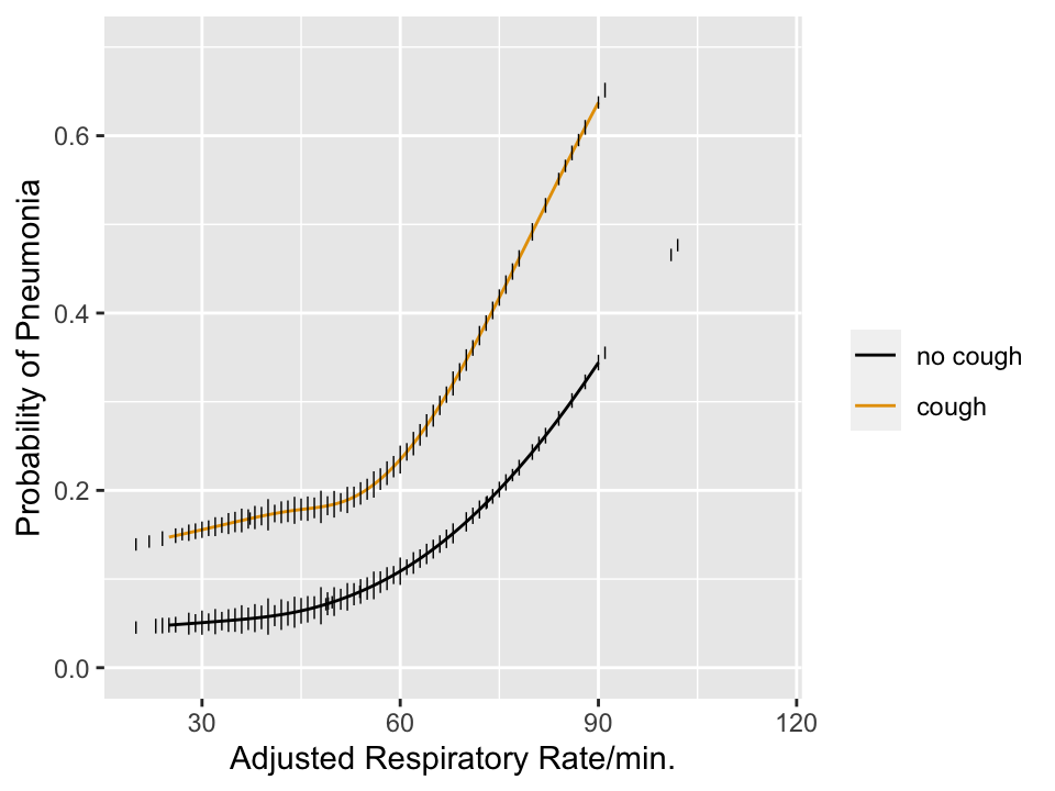
* A simple 2-predictor example related to diagnosis of pneumonia will suffice
* It is **never** appropriate to dichotomize an input variable other than time. Dichotomization, if it must be done, should **only** be done on $\hat{Y}$. In other words, dichotomization is done as late as possible in decision making. When more than one continuous predictor variable is relevant to outcomes, the example below shows that it is mathematically incorrect to do a one-time dichotomization of a predictor. As an analogy, suppose that one is using body mass index (BMI) by itself to make a decision. One would never categorize height and categorize weight to make the decision based on BMI. One could categorize BMI, if no other outcome predictors existed for the problem.
```{r pneuwho,w=5,h=3.75,cap='Estimated risk of pneumonia with respect to two predictors in WHO ARI study from @har98dev. Tick marks show data density of respiratory rate stratified by cough. Any cutpoint for the rate **must** depend on cough to be consistent with optimum decision making, which must be risk-based.',scap='Risk of pneumonia with two predictors'}
#| label: fig-info-pneuwho
require(rms)
getHdata(ari)
r <- ari[ari$age >= 42, Cs(age, rr, pneu, coh, s2)]
abn.xray <- r$s2==0
r$coh <- factor(r$coh, 0:1, c('no cough','cough'))
f <- lrm(abn.xray ~ rcs(rr,4)*coh, data=r)
anova(f)
dd <- datadist(r); options(datadist='dd')
p <- Predict(f, rr, coh, fun=plogis, conf.int=FALSE)
ggplot(p, rdata=r,
       ylab='Probability of Pneumonia',
       xlab='Adjusted Respiratory Rate/min.',
       ylim=c(0,.7), legend.label='')
```
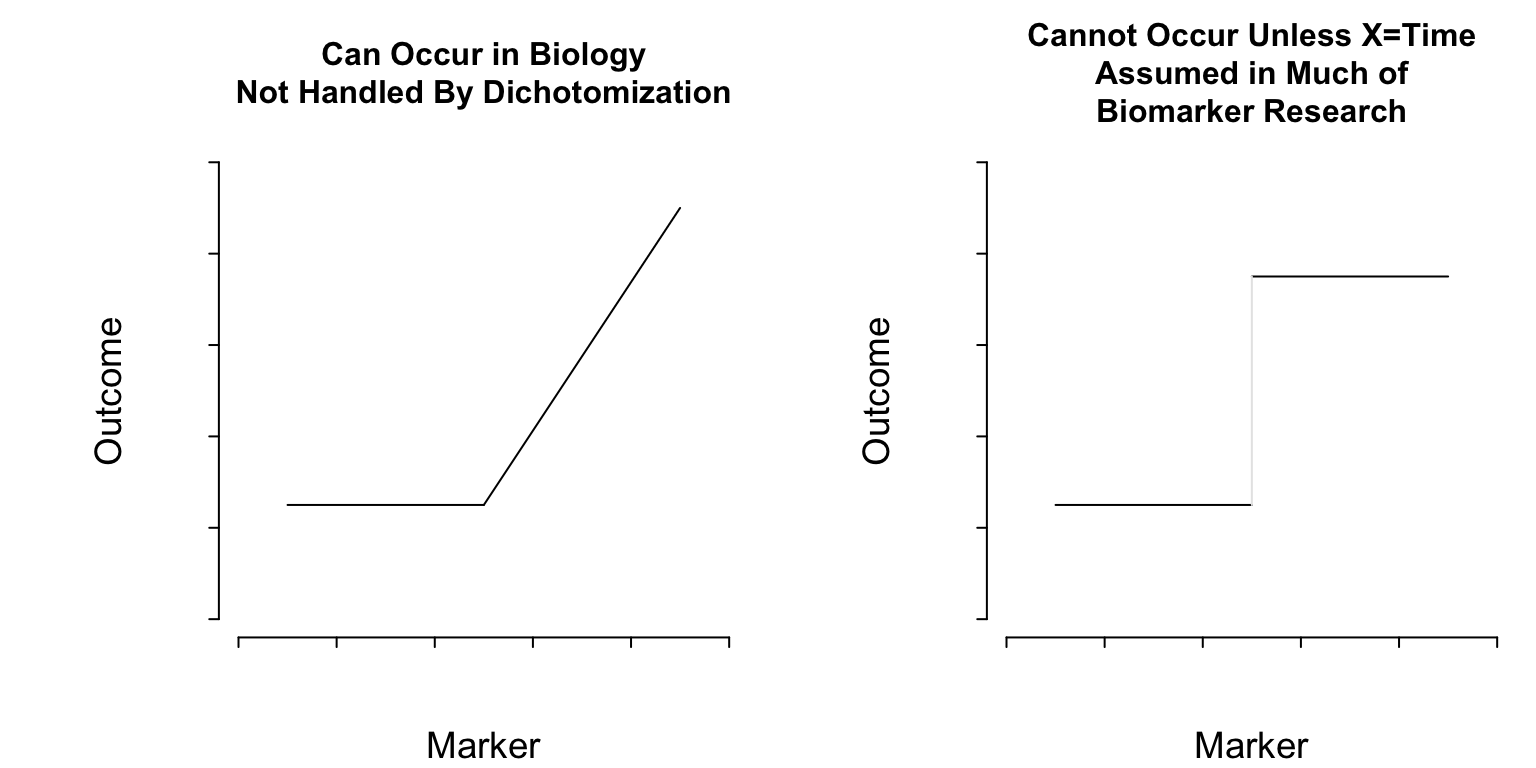
### What Kinds of True Thresholds Exist?
`r quoteit("Natura non facit saltus<br>(Nature does not make jumps)", "Gottfried Wilhelm Leibniz")`
```{r thresholds,echo=FALSE}
#| label: fig-info-thresholds
#| column: page-inset-left
#| fig-width: 8
#| fig-height: 4
#| fig-cap: "Two kinds of thresholds. The pattern on the left represents a discontinuity in the first derivative (slope) of the function relating a marker to outcome. On the right there is a lowest-order discontinuity."
#| fig-scap: "Two kinds of thresholds"
spar(top=3,mfrow=c(1,2))
plot(0:1, 0:1, type='n', axes=FALSE, xlab='Marker', ylab='Outcome',
main='Can Occur in Biology\nNot Handled By Dichotomization',
cex.main=1)
axis(1, labels=FALSE)
axis(2, labels=FALSE)
lines(c(.1, .5), c(.25, .25))
lines(c(.5, .9), c(.25, .9))
plot(0:1, 0:1, type='n', axes=FALSE, xlab='Marker', ylab='Outcome',
main='Cannot Occur Unless X=Time\nAssumed in Much of\nBiomarker Research',
cex.main=1)
axis(1, labels=FALSE)
axis(2, labels=FALSE)
lines(c(.1, .5), c(.25, .25))
lines(c(.5, .9), c(.75, .75))
lines(c(.5, .5), c(.25, .75), col=gray(.9))
```
**What Do Cutpoints Really Assume?** <br>
Cutpoints assume discontinuous relationships of the type in the right
plot of @fig-info-thresholds, and they assume that the
true cutpoint is known. Beyond the molecular level, such patterns do
not exist unless $X=$time and the discontinuity is caused by an event.
Cutpoints assume homogeneity of outcome on either side of the cutpoint.
### Cutpoints are Disasters
* Prognostic relevance of S-phase fraction in breast cancer: 19 different cutpoints used in literature
* Cathepsin-D content and disease-free survival in node-negative breast cancer: 12 studies, 12 cutpoints
* ASCO guidelines: neither cathepsin-D nor S-phrase fraction recommended as prognostic markers (@hol04con)
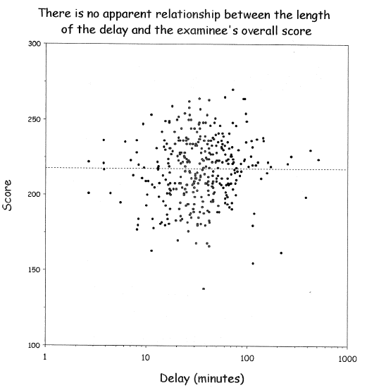
Cutpoints may be found that result in both increasing and
decreasing relationships with **any** dataset with zero
correlation
| Delay | Mean Score |
|-----|-----|
| 0-11 | 210 | 0-3.8| 220 |
| 11-20 | 215 | 3.8-8| 219 |
| 21-30 | 217 | 8-113| 217 |
| 31-40 | 218 | 113-170| 215 |
| 41- | 220 | 170-| 210 |
@wai06fin; See "Dichotomania" (@sen05dic) and @roy06dic
<img src="images/wai06fin.png" width="80%">
@wai06fin
**In fact, virtually all published cutpoints are analysis artifacts** caused by finding a threshold that minimizes $P$-values
when comparing outcomes of subjects below with those above the
"threshold". Two-sample statistical tests suffer the least loss of
power when cutting at the median because this balances the sample
sizes. That this method has nothing to do with biology can be readily
seen by adding observations on either tail of the marker, resulting in
a shift of the median toward that tail even though the relationship
between the continuous marker and the outcome remains unchanged.
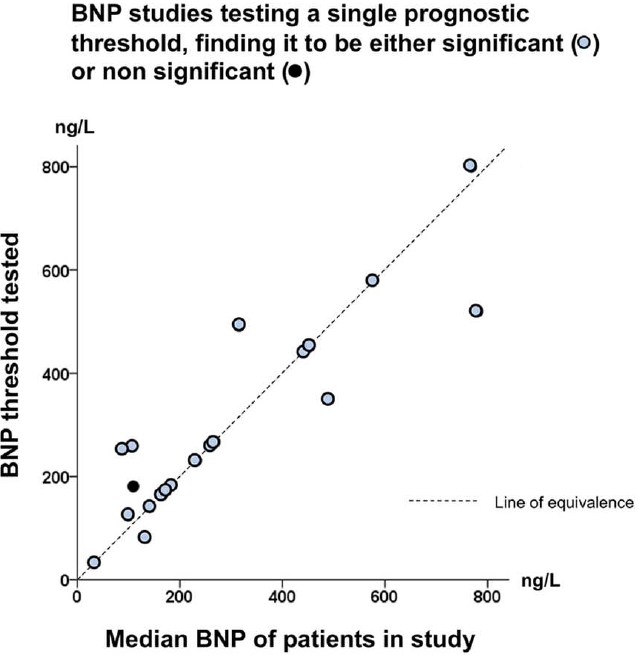
```{r gia14opt,out.width="600px"}
#| label: fig-info-gia14opt
#| fig-cap: "Thresholds in cardiac biomarkers"
knitr::include_graphics('images/gia14opt-fig2c.png')
```
In "positive" studies: threshold 132--800 ng/L, correlation with study
median $r=0.86$ (@gia14opt)
#### Lack of Meaning of Effects Based on Cutpoints
* Researchers often use cutpoints to estimate the high:low effects of risk factors (e.g., BMI vs. asthma)
* Results in inaccurate predictions, residual confounding, impossible to interpret
* high:low represents unknown mixtures of highs and lows
* Effects (e.g., odds ratios) will vary with population
* If the true effect is monotonic, adding subjects in the low range or high range or both will increase odds ratios (and all other effect measures) arbitrarily
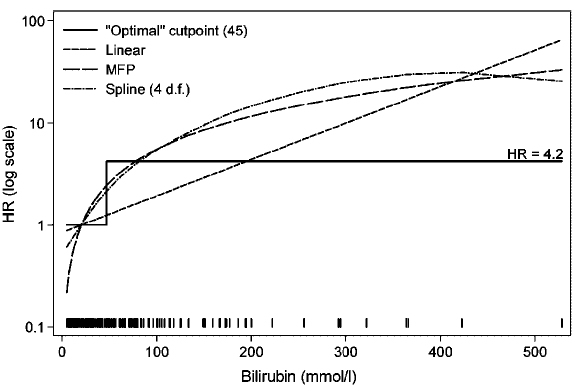
<img src="images/roy06dicb.png" width="80%">
@roy06dic, @nag11ana, @gia14opt
Does a physician ask the nurse "Is this patient's bilirubin $>$ 45"
or does she ask "What is this patient's bilirubin level?".
Imagine how a decision support system would trigger vastly different
decisions just because bilirubin was 46 instead of 44.
As an example of how a hazard ratio for a dichotomized continuous
predictor is an arbitrary function of the entire distribution of the
predictor within the two categories, consider a Cox model analysis of
simulated age where the true effect of age is linear. First compute
the $\geq 50:< 50$ hazard ratio in all subjects, then in just the
subjects having age $< 60$, then in those with age $< 55$. Then
repeat including all older subjects but excluding subjects with age
$\leq 40$. Finally, compute the hazard ratio when only those age 40
to 60 are included. Simulated times to events have an
exponential distribution, and proportional hazards holds.
```{r coxsim}
require(survival)
set.seed(1)
n <- 1000
age <- rnorm(n, mean=50, sd=12)
# describe(age)
cens <- 15 * runif(n)
h  <- 0.02 * exp(0.04 * (age - 50))
dt <- -log(runif(n))/h
e  <- ifelse(dt <= cens,1,0)
dt <- pmin(dt, cens)
S  <- Surv(dt, e)
d  <- data.frame(age, S)
# coef(cph(S ~ age))   # close to true value of 0.04 used in simulation
g <- function(sub=1 : n)
       exp(coef(cph(S ~ age >= 50, data=d, subset=sub)))
d <- data.frame(Sample=c('All', 'age < 60', 'age < 55', 'age > 40',
                         'age 40-60'),
                'Hazard Ratio'=c(g(), g(age < 60), g(age < 55),
                                 g(age > 40), g(age > 40 & age < 60)))
d
```
See
[this](https://bmcmedresmethodol.biomedcentral.com/articles/10.1186/1471-2288-12-21)
for excellent graphical examples of the harm of categorizing
predictors, especially when using quantile groups.
### Categorizing Outcomes {#sec-info-catoutcomes}
* Arbitrary, low power, can be difficult to interpret
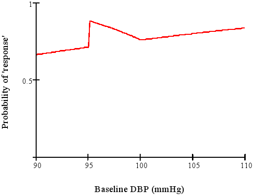
* Example: "The treatment is called successful if either the patient has gone down from a baseline diastolic blood pressure of $\geq 95$ mmHg to $\leq 90$ mmHg or has achieved a 10\% reduction in blood pressure from baseline."
* Senn derived the response probabililty function for this discontinuous concocted endpoint
<img src="images/dichotomaniaFig3.png" width="80%">
@sen05dic after Goetghebeur [1998]
Is a mean difference of 5.4mmHg more difficult to interpret than
A:17\% vs. B:22\% hit clinical target?
"Responder" analysis in clinical trials results in huge information loss and arbitrariness. Some issue:
* Responder analyses use cutpoints on continuous or ordinal variables and cite earlier data supporting their choice of cutpoints. No example has been produced where the earlier data actually support the cutpoint.
* Many responder analyses are based on change scores when they should be based solely on the follow-up outcome variable, adjusted for baseline as a covariate.
* The cutpoints are always arbitrary.
* There is a huge power loss (see @sec-info-catoutcomes).
* The responder probability is often a function of variables that one does not want it to be a function of (see graph above).
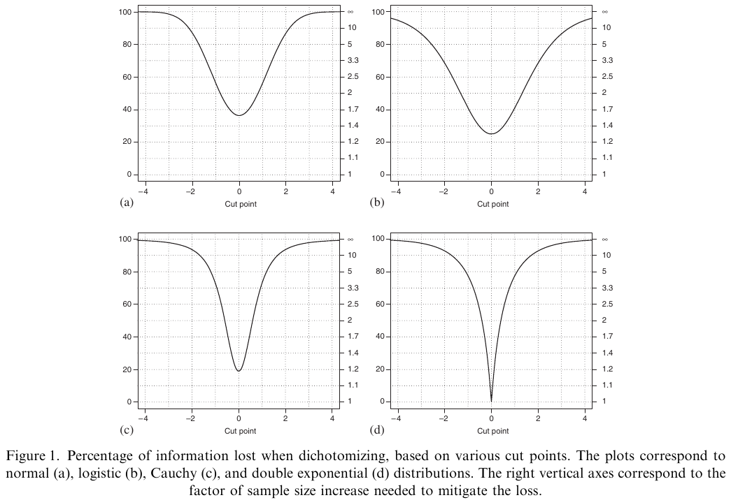
@fed09con is one of the best papers quantifying the information
and power loss from categorizing continuous outcomes. One of their
examples is that a clinical trial of 100 subjects with continuous $Y$
is statistically equivalent to a trial of 158 dichotomized
observations, assuming that the dichotomization is at the
**optimum** point (the population median). They show that it is
very easy for dichotomization of $Y$ to raise the needed sample size
by a factor of 5.
```{r fed09con,out.width="600px"}
#| label: fig-info-fed09con
#| fig-cap: "Power loss from dichotomizing the response variable"
#| fig.width: 5
knitr::include_graphics('images/fed09conFig1.png')
```
@fed09con
### Classification vs. Probabilistic Thinking
`r mrg(movie("https://youtu.be/1yYrDVN_AYc"))`
`r quoteit("**Number needed to treat**. The only way, we are told, that physicians can understand probabilities: odds being a difficult concept only comprehensible to statisticians, bookies, punters and readers of the sports pages of popular newspapers.", "@sensta")`
* Many studies attempt to classify patients as diseased/normal
* Given a reliable estimate of the probability of disease and the consequences of +/- one can make an optimal decision
* Consequences are known at the point of care, not by the authors; categorization **only** at point of care
* Continuous probabilities are self-contained, with their own "error rates"
* Middle probs. allow for "gray zone", deferred decision
| Patient | Prob[disease] | Decision | Prob[error] |
|-----|-----|-----|-----|
| 1 | 0.03 | normal | 0.03 |
| 2 | 0.40 | normal | 0.40 |
| 3 | 0.75 | disease | 0.25 |
Note that much of diagnostic research seems to be aimed at
making optimum decisions for groups of patients. The optimum decision
for a group (if such a concept even has meaning) is not optimum for
individuals in the group.
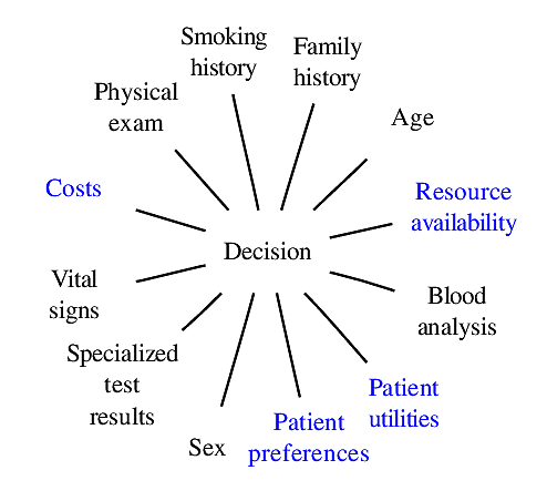
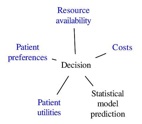
### Components of Optimal Decisions
<img src="images/mdDec.png" width="80%">
Statistical models reduce the dimensionality of the problem _but not to unity_
<img src="images/mdDecm.png" width="80%">
## Problems with Classification of Predictions
`r mrg(movie("https://youtu.be/FDTwEZ3KcyA"))`
* Feature selection / predictive model building requires choice of a scoring rule, e.g. correlation coefficient or proportion of correct classifications
* Prop. classified correctly is a discontinuous **improper scoring rule**
+ Maximized by bogus model \smaller{(example below)}
* Minimum information
+ low statistical power
+ high standard errors of regression coefficients
+ arbitrary to choice of cutoff on predicted risk
+ forces binary decision, does not yield a "gray zone" $\rightarrow$ more data needed
* Takes analyst to be provider of utility function and not the treating physician
* Sensitivity and specificity are also improper scoring rules
See
[bit.ly/risk-thresholds](https://bmcmedicine.biomedcentral.com/articles/10.1186/s12916-019-1425-3):
Three Myths About Risk Thresholds for Prediction Models by Wynants~\etal
### Example: Damage Caused by Improper Scoring Rule
* Predicting probability of an event, e.g., Prob[disease]
* $N=400$, 0.57 of subjects have disease
* Classify as diseased if prob. $>0.5$
| Model | $c$ | $\chi^{2}$ | Proportion |
|-----|-----|-----|-----|
| | Index | | Correct |
| age | .592 | 10.5 | .622 |
| sex | .589 | 12.4 | .588 |
| age+sex | .639 | 22.8 | .600 |
| constant |.500 | 0.0 | .573 |
Adjusted Odds Ratios:<br>
| age (IQR 58y:42y) | 1.6 (0.95CL 1.2-2.0) |
|-----|-----|
| sex (f:m) | 0.5 (0.95CL 0.3-0.7) |
Test of sex effect adjusted for age $(22.8-10.5)$:<br>$P=0.0005$
#### Example where an improper accuracy score resulted in incorrect original analyses and incorrect re-analysis
@mic05pre used an improper accuracy score (proportion
classified "correctly") and
claimed there was really no signal in all the published gene
microarray studies they could analyze. This is true from the
standpoint of repeating the original analyses (which also used improper
accuracy scores) using multiple splits of the data, exposing the
fallacy of using single data-splitting for validation. @ali09fac
used a semi-proper accuracy score ($c$-index) and they repeated 10-fold
cross-validation 100 times instead of using highly volatile data
splitting. They showed that the gene microarrays did indeed have
predictive signals.^[@ali09fac also used correct statistical models for time-to-event data that properly accounted for variable follow-up/censoring.]
| @mic05pre | @ali09fac |
|-----|-----|
| % classified correctly | $c$-index |
| Single split-sample validation | Multiple repeats of 10-fold CV |
| Wrong tests | Correct tests |
| (censoring, failure times) | |
| 5 of 7 published microarray | 6 of 7 have signals |
| studies had no signal | |
## Value of Continuous Markers
* Avoid arbitrary cutpoints
* Better risk spectrum
* Provides gray zone
* Increases power/precision
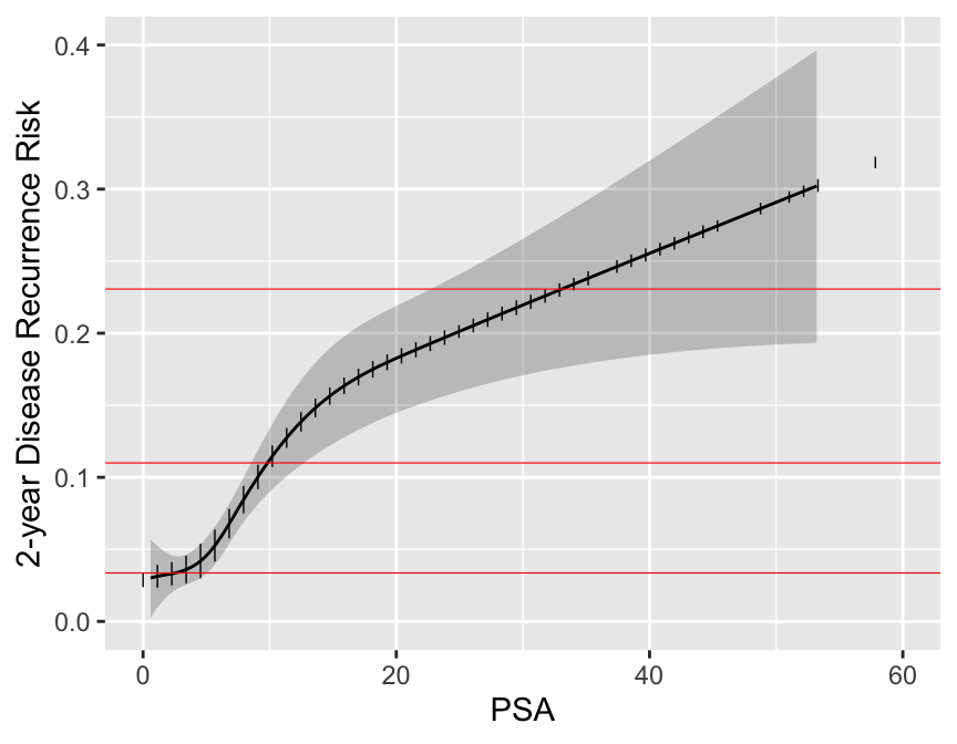
### Prognosis in Prostate Cancer
```{r psa,w=4.5,h=3.5,cap='Relationship between post-op PSA level and 2-year recurrence risk. Horizontal lines represent the only prognoses provided by the new staging system. Data are courtesy of M Kattan from JNCI 98:715; 2006. Modification of AJCC staging by Roach _et al._ 2006.',scap='Continuous PSA vs. risk'}
#| label: fig-info-psa
load('~/doc/Talks/infoAllergy/kattan.rda')
attach(kattan)
t   <- t.stg
gs  <- bx.glsn
psa <- preop.psa
t12 <- t.stg %in% Cs(T1C,T2A,T2B,T2C)

s <- score.binary(t12 & gs<=6 & psa<10,
                  t12 & gs<=6 & psa >=10 & psa < 20,
                  t12 & gs==7 & psa < 20,
                  (t12 & gs<=6 & psa>=20) |
                  (t12 & gs>=8 & psa<20),
                  t12 & gs>=7 & psa>=20,
                  t.stg=='T3')
levels(s) <- c('none','I', 'IIA', 'IIB', 'IIIA', 'IIIB', 'IIIC')
u <- is.na(psa + gs) | is.na(t.stg)
s[s=='none'] <- NA
s <- s[drop=TRUE]
s3 <- s
levels(s3) <- c('I','II','II','III','III','III')
# table(s3)
units(time.event) <- 'month'
dd <- datadist(data.frame(psa, gs)); options(datadist='dd')
S <- Surv(time.event, event=='YES')
label(psa) <- 'PSA'; label(gs) <- 'Gleason Score'
f <- cph(S ~ rcs(sqrt(psa), 4), surv=TRUE, x=TRUE, y=TRUE)
p <- Predict(f, psa, time=24, fun=function(x) 1 - x)
h <- cph(S ~ s3, surv=TRUE)
z <- 1 - survest(h, times=24)$surv
ggplot(p, rdata=data.frame(psa), xlim=c(0,60),
       ylab='2-year Disease Recurrence Risk') +
  geom_hline(yintercept=unique(z), col='red', size=0.2)
```
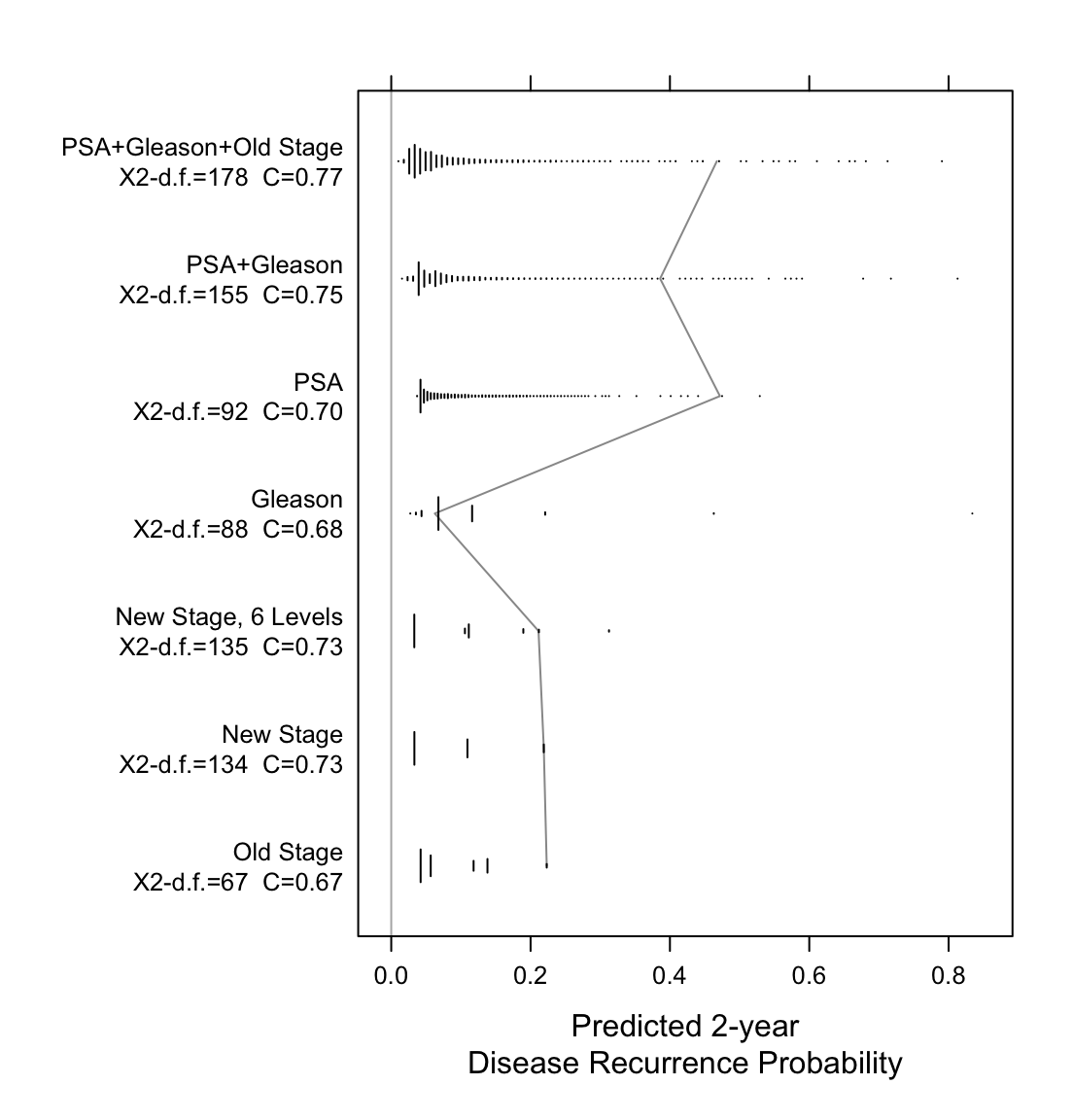
Now examine the entire spectrum of estimated prognoses from variables
models and from discontinuous staging systems.
```{r spectrum,w=5.75,h=6,cap='Prognostic spectrum from various models with model $\\chi^2$ - d.f., and generalized $c$-index. The mostly vertical segmented line connects different prognostic estimates for the same man.',scap='Prognostic spectrum from various models'}
#| label: fig-info-spectrum
d <- data.frame(S, psa, s3, s, gs, t.stg, time.event, event, u)
f <- cph(S ~ rcs(sqrt(psa),4) + pol(gs,2), surv=TRUE, data=d)
g <- function(form, lab) {
  f <- cph(form, surv=TRUE, data=subset(d, ! u))
  cat(lab,'\n'); print(coef(f))
  s <- f$stats
  cat('N:', s['Obs'],'\tL.R.:', round(s['Model L.R.'],1),
      '\td.f.:',s['d.f.'],'\n\n')
  prob24 <- 1 - survest(f, times=24)$surv
  prn(sum(!is.na(prob24)))
  p2 <<- c(p2, prob24[2])  # save est. prognosis for one subject
  p1936 <<- c(p1936, prob24[1936])
  C <- rcorr.cens(1-prob24, S[!u,])['C Index']
  data.frame(model=lab, chisq=s['Model L.R.'], d.f.=s['d.f.'],
             C=C, prognosis=prob24)
}
p2 <- p1936 <- NULL
w <-          g(S ~ t.stg, 'Old Stage')
w <- rbind(w, g(S ~ s3, 'New Stage'))
w <- rbind(w, g(S ~ s, 'New Stage, 6 Levels'))
w <- rbind(w, g(S ~ pol(gs,2), 'Gleason'))
w <- rbind(w, g(S ~ rcs(sqrt(psa),4), 'PSA'))
w <- rbind(w, g(S ~ rcs(sqrt(psa),4) + pol(gs,2), 'PSA+Gleason'))
w <- rbind(w, g(S ~ rcs(sqrt(psa),4) + pol(gs,2) + t.stg,
                'PSA+Gleason+Old Stage'))
w$z <- paste(w$model, '\n',
             'X2-d.f.=',round(w$chisq-w$d.f.),
             '  C=', sprintf("%.2f", w$C), sep='')
w$z <- with(w, factor(z, unique(z)))
require(lattice)
stripplot(z ~ prognosis, data=w, lwd=1.5,
          panel=function(x, y, ...) {
            llines(p2, 1:7, col=gray(.6))
            ## llines(p1936, 1:7, col=gray(.8), lwd=2)
            ## panel.stripplot(x, y, ..., jitter.data=TRUE, cex=.5)
            for(iy in unique(unclass(y))) {
              s <- unclass(y)==iy
              histSpike(x[s], y=rep(iy,sum(s)), add=TRUE, grid=TRUE)
            }
            panel.abline(v=0, col=gray(.7))
          },
          xlab='Predicted 2-year\nDisease Recurrence Probability')
```
## Harm from Ignoring Information
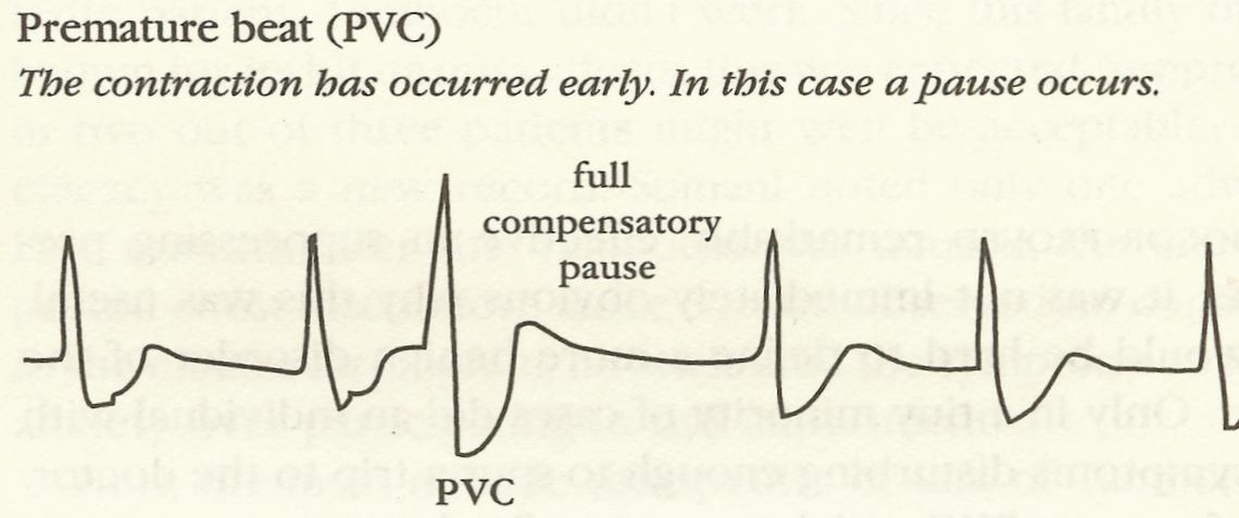
### Case Study: Cardiac Anti-arrhythmic Drugs {#sec-pvcs}
* Premature ventricular contractions were observed in patients surviving acute myocardial infarction
* Frequent PVCs $\uparrow$ incidence of sudden death
<img src="images/pvcDeadlyMedicine.png" width="70%">
@moo95dea, p. 46
**Arrhythmia Suppression Hypothesis**
`r quoteit("Any prophylactic program against sudden death must involve the use of anti-arrhythmic drugs to subdue ventricular premature complexes.", "Bernard Lown<br> <small> Widely accepted by 1978")`</small>
<img src="images/mul83risFig2.jpg" width="70%">
@moo95dea, p. 49; @mul83ris
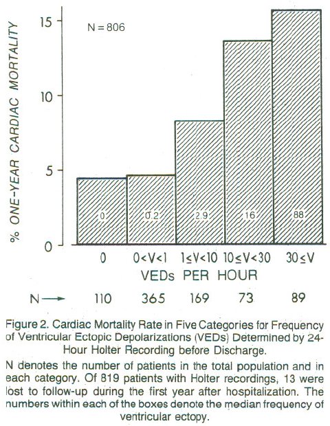
Are PVCs independent risk factors for sudden cardiac death?
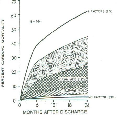
Researchers developed a 4-variable model for prognosis after acute MI
* left ventricular ejection fraction (EF) $< 0.4$
* PVCs $>$ 10/hr
* Lung rales
* Heart failure class II,III,IV
<img src="images/mul83risFig3b.jpg" width="80%">
@mul83ris
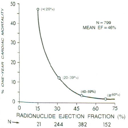
**Dichotomania Caused Severe Problems**
* EF alone provides same prognostic spectrum as the researchers' model
* Did not adjust for EF!; PVCs $\uparrow$ when EF$<0.2$
* Arrhythmias prognostic in isolation, not after adjustment for continuous EF and anatomic variables
* Arrhythmias predicted by local contraction abnorm., then global function (EF)
<img src="images/mul83risFig1.jpg" width="80%">
@mul83ris; @cal82pro
### CAST: Cardiac Arrhythmia Suppression Trial
* Randomized placebo, moricizine, and Class IC anti-arrhythmic drugs flecainide and encainide
* Cardiologists: unethical to randomize to placebo
* Placebo group included after vigorous argument
* Tests design as one-tailed; did not entertain possibility of harm
* Data and Safety Monitoring Board recommended early termination of flecainide and encainide arms
* Deaths $\frac{56}{730}$ drug, $\frac{22}{725}$ placebo, RR 2.5
@inv89pre
**Conclusions: Class I Anti-Arrhythmics**
<img src="images/deadlyMedicine.jpg" width="50%">
Estimate of excess deaths from Class I anti-arrhythmic drugs: 24,000--69,000<br>
Estimate of excess deaths from Vioxx: 27,000--55,000
Arrhythmia suppression hypothesis refuted; PVCs merely indicators of
underlying, permanent damage
@moo95dea, pp. 289,49; D Graham, FDA
## Case Study in Faulty Dichotomization of a Clinical Outcome: Statistical and Ethical Concerns in Clinical Trials for Crohn's Disease {#sec-crohn}
### Background
Many clinical trials are underway for studying treatments for Crohn's disease.
The primary endpoint for these studies is a
discontinuous, information--losing transformation of the Crohn's
Disease Activity Index
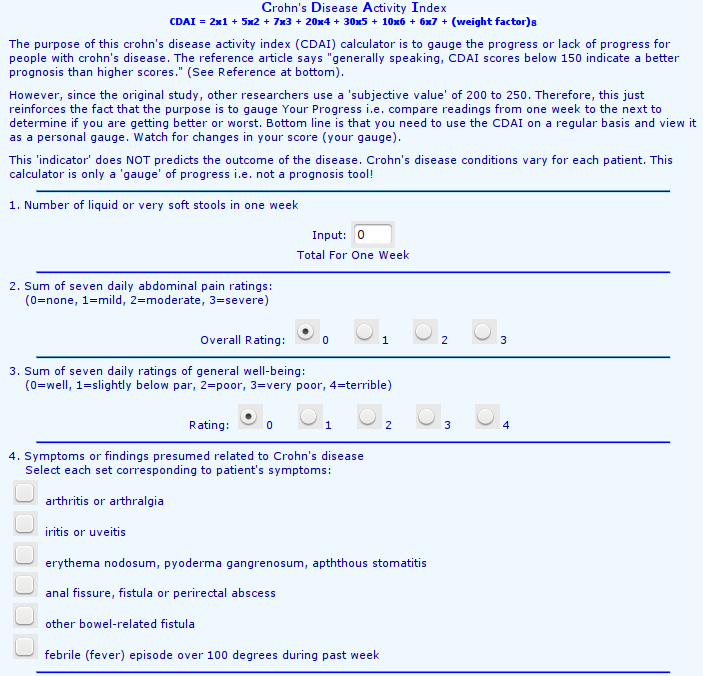
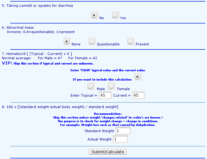
(CDAI) @bes76dev, which was developed in 1976 by
using an exploratory stepwise regression method to predict four levels
of clinicians' impressions of patients' current
status^[Ordinary least squares regression was used for the ordinal response variable. The levels of the response were assumed to be equally spaced in severity on a numerical scale of 1, 3, 5, 7 with no justification.]. The first
level ("very well") was assumed to indicate the patient was in
remission. The model was overfitted and was not validated. The
model's coefficients were scaled and rounded, resulting in the
following scoring system (see [www.ibdjohn.com/cdai](http://www.ibdjohn.com/cdai)).
<img src="images/cdai-score1.png" width="80%"><br>
<img src="images/cdai-score2.png" width="80%">
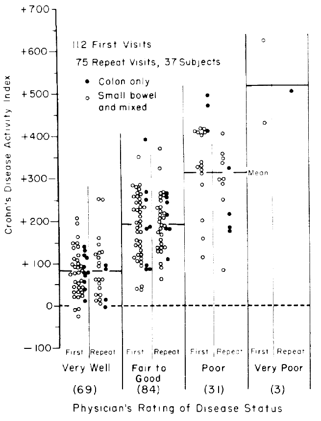
The original authors plotted the predicted scores against the four
clinical categories as shown below.
<img src="images/bes76devFig1.png" width="75%">
The authors arbitrarily assigned a cutoff of 150, below which
indicates "remission."^[However, the authors intended for CDAI to be used on a continuum: "... a numerical index was needed, the numerical value of which would be proportional to degree of illness ... it could be used as the principal measure of response to the therapy under trial ... the CDAI appears to meet those needs. ... The data presented ... is an accurate numerical expression of the physician's over-all assessment of degree of illness in a large group of patients ... we believe that it should be useful to all physicians who treat Crohn's disease as a method of assessing patient progress.".] It can be seen that
"remission" includes a
good number of patients actually classified as "fair to good" or
"poor." A cutoff only exists when there is a break in the
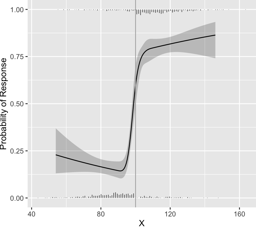
distribution of scores. As an example, data were simulated from a
population in which every patient having a score below 100 had a
probability of response of 0.2 and every patient having a score above
100 had a probability of response of 0.8. Histograms showing the
distributions of non-responders (just above the $x$-axis) and
responders (at the top of the graph) appear in the figure below. A
flexibly fitted logistic regression model relating observed scores to
actual response status is shown, along with 0.95 confidence intervals
for the fit.
```{r cutpointExists,w=4.5,h=4}
require(rms)
set.seed(4)
n <- 900
X <- rnorm(n, 100, 20)
dd <- datadist(X); options(datadist='dd')

p <- ifelse(X < 100, .2, .8)
y <- ifelse(runif(n) <= p, 1, 0)

f <- lrm(y ~ rcs(X, c(90,95,100,105,110)))
hs <- function(yval, side)
  histSpikeg(yhat ~ X, data=subset(data.frame(X, y), y == yval),
             side = side, ylim = c(0, 1),
             frac = function(f) .03 * f / max(f))
ggplot(Predict(f, fun=plogis), ylab='Probability of Response') +
  hs(0, 1) + hs(1, 3) + geom_vline(xintercept=100, col=gray(.7))
```
One can see that the fitted curves justify the use of a cut-point of
100. However, the original scores from the development of CDAI do not
justify the existence of a cutoff. The fitted logistic model used to
relate "very well" to the other three categories is shown below.
```{r devlogistread,echo=FALSE}
d <- read.table(textConnection(
"0.29017806553 -26.5670446561
0.251361744241 -11.2913339428
0.314187070796 -8.22259324454
0.416584193946 8.4673672441
0.236463771182 18.8611965218
0.307040274389 18.4124441893
0.369895819955 22.6370621076
0.346460975923 26.2542778789
0.291689016145 31.2268163515
0.228924127615 30.4698300936
0.401595563849 35.1522660482
0.378221157841 41.0812362598
0.307644654634 41.5299885923
0.229286755762 44.3403567354
0.292202739353 50.8767290941
0.253114446954 55.7495448261
0.331623440888 58.7185627838
0.394267453368 54.8520401611
0.402471915205 68.6727054326
0.449704231417 75.3088005319
0.39481139559 75.6578301238
0.35572310319 80.5306458558
0.300709391314 76.2561665672
0.237974721796 76.6550575294
0.167307561552 73.6361782015
0.395143804725 88.3724795455
0.340311406922 91.0332635778
0.293199966759 89.0206773592
0.246179183633 90.475722801
0.207121110247 96.5044157532
0.301283552547 98.2178337501
0.277939365552 105.302681182
0.23882085414 109.019619694
0.278271774687 118.017330604
0.380215612653 117.36913279
0.434927134407 110.084839877
0.39614103213 126.516427811
0.396443222253 138.075200012
0.302310998965 137.517659235
0.223832224044 135.704518498
0.216232142452 145.001397629
0.294710917374 146.814538367
0.295103764533 161.840942229
0.280175572461 190.837595473
0.272726585932 205.913860705
0.729864694372 -8.55349142913
0.730317979557 8.78466687316
0.651688109574 1.1921400349
0.644088027983 10.4890191664
0.581323139453 9.7320329085
0.652262270808 23.1538072178
0.573843933911 23.6524209206
0.636971450588 38.2799338204
0.621559754319 48.7825515423
0.676694342245 57.6805397116
0.621801506418 58.0295693035
0.56690867059 58.3785988955
0.724410162654 82.8106703332
0.740335582131 91.9579653539
0.61477558606 89.2881156179
0.630670786525 97.2795334185
0.615319528281 110.093905581
0.560608006527 117.378198494
0.639117000461 120.347216451
0.678416825946 123.56554126
0.624037713327 143.564483595
0.624370122463 156.279133017
0.618945809756 248.799171999
0.697303708628 245.988803856
1.38326017814 383.82376272
1.27238662204 342.910241979
1.60225736022 360.46597717
1.60101838071 313.075011143
1.17650169604 275.311822433
1.23136431286 273.806915621
1.29421985842 278.031533539
1.27823400092 266.572484078
1.24662491406 257.524911798
1.30929914556 254.814266396
1.19155076416 250.938678069
1.24644359999 250.589648477
1.28547145437 243.405078305
1.22255547077 236.868705946
1.29310175497 235.264076394
1.29282978386 224.861181412
1.36337606805 223.25655186
1.19073485083 219.729993125
1.24562768666 219.380963533
1.29252759374 213.302409211
1.30012767533 204.005530079
1.28414181782 192.546480618
1.23696993964 188.222139959
1.28386984671 182.143585637
1.2445095832 176.613506388
1.2521096648 167.316627256
1.29916066693 167.017459034
1.23591227421 147.766437254
1.28290283832 145.155514592
1.21989619769 135.151510573
1.29041226288 132.3910038
1.29798212545 121.938247448
1.25853120491 112.940536539
1.30555198803 111.485491097
1.19561522132 106.40416418
1.25029652406 97.9639940469
1.29749862126 103.444211926
1.29725686916 94.1971941647
1.30491738878 87.2120694735
1.40686122674 86.5638716599
1.45367047678 77.0176856769
1.38306375456 76.3105607893
1.31927141961 36.2537490462
1.31124827185 29.3683470956
1.23286015397 31.0228380185
1.40355224489 259.995316053
1.40303852169 240.34540331
1.39341376627 172.198508692
1.46417158355 178.68501968
1.67017459034 258.300029464
1.62306315018 256.287443245
1.61491912637 244.778532414
1.63042147967 237.743546352
1.66996305726 250.208888922
1.71719537347 256.844984022
1.71689318335 245.28621182
1.7244026079 232.521701028
1.56726374398 221.960156232
1.61434496513 222.816865231
1.62194504673 213.519986099
1.61389167995 205.478706928
1.59796626047 196.331411908
1.59775472739 188.240271367
1.67644503539 198.144552645
1.6767170065 208.547447627
1.7315191853 204.730786374
1.62891052906 179.949685345
1.69161497956 178.394917162
1.70714755188 172.515808321
1.76197994969 169.855024289
1.62085716228 171.908406174
1.57359462706 164.116433854
1.63620842053 159.094034011
1.62013190599 144.16735289
1.63560404028 135.976489608
1.69031556204 128.692196696
1.62749023548 125.623455997
1.57262761867 127.128362809
1.58022770026 117.831483678
1.62730892141 118.688192676
1.73664130788 100.65197519
1.62652322709 88.6353849524
1.62628147499 79.3883671912
1.64123988607 51.547591167
2.38189276783 481.520318508
2.38122794956 456.091019665
2.26224058867 404.824465312
2.32497525818 404.42557435
2.37971699895 398.297158657
2.33254512076 393.972817998
2.28534302356 388.492600119
2.2384733355 395.727031662
2.17582932302 399.593554285
2.62260231024 388.660315638
2.61355171606 342.475088202
2.62893319332 330.81659326
2.62078916951 319.307682428
2.72243081735 307.100712413
2.27580892519 323.813337161
2.2834694448 316.82821247
2.27538585901 307.631056079
2.28295572159 297.178299727
2.22064411825 313.759471772
2.56492932529 282.668640975
2.62769421381 283.425627233
2.61958040901 273.072593622
2.29007229899 269.387385073
2.61858318161 234.928645357
2.71962044921 199.604130939
2.28792674911 187.320102442
2.29465047935 144.502783927
2.29350215688 100.579449561
2.62988509221 67.2267256945
2.72664636956 168.345584625
2.73421623214 157.892828273
3.27140450414 605.344232324
3.71527646619 483.446780542
3.28198115845 409.901259377"), col.names=c('x','y'))
```
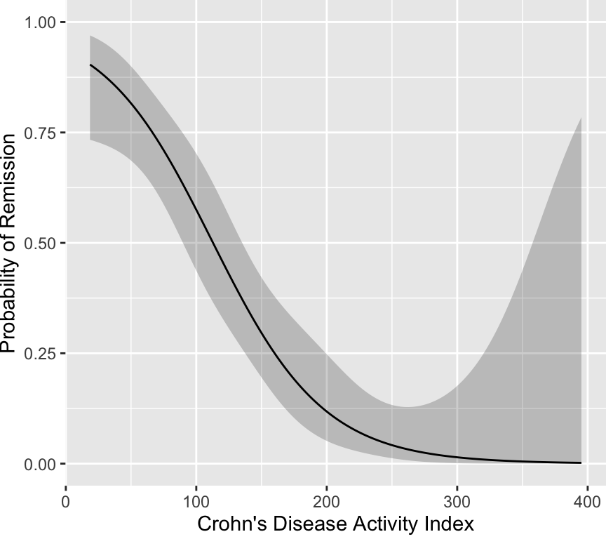
```{r devlogist,w=4.5,h=4}
# Points from published graph were defined in code not printed
g <- trunc(d$x)
g <- factor(g, 0:3, c('very well', 'fair to good', 'poor', 'very poor'))
remiss <- 1 * (g == 'very well')
CDAI <- d$y
label(CDAI) <- "Crohn's Disease Activity Index"
label(remiss) <- 'Remission'
dd <- datadist(CDAI,remiss); options(datadist='dd')
f <- lrm(remiss ~ rcs(CDAI,4))
ggplot(Predict(f, fun=plogis), ylab='Probability of Remission')
```
It is readily seen that no cutoff exists, and one would have to be
below CDAI of 100 for the probability of remission to fall below even
0.5. The probability does not exceed 0.9 until the score falls below
25. Thus there is no clinical justification for the 150 cut-point.
### Loss of Information from Using Cut-points
The statistical analysis plan in the Crohn's disease protocols specify
that efficacy will be judged by comparing two proportions after
classifying patients' CDAIs as above or below the cutoff of 150.
Even if one could justify a certain cutoff from the data, the use of the
cutoff is usually not warranted. This is because of the huge loss of
statistical efficiency, precision, and power from dichotomizing
continuous variables as discussed in more detail in
@sec-info-catoutcomes.
If one were forced to dichotomize a continuous
response $Y$, the cut-point that loses the least efficiency is the
population median of $Y$ combining treatment groups. That implies a
statistical efficiency of $\frac{2}{\pi}$ or 0.637 when compared to
the efficient two-sample $t$-test if the data are normally
distributed^[Note that the efficiency of the Wilcoxon test compared to the $t$-test is $\frac{3}{\pi}$ and the efficiency of the sign test compared to the $t$-test is $\frac{2}{\pi}$. Had analysis of covariance been used instead of a simple two-group comparison, the baseline level of CDAI could have been adjusted for as a covariate. This would have increased the power of the continuous scale approach to even higher levels.]. In other words,
the optimum cut-point would require
studying 158 patients after dichotomizing the response variable to get
the same power as analyzing the continuous response variable in 100
patients.
### Ethical Concerns and Summary
The CDAI was based on a sloppily-fit regression model predicting a
subjective clinical impression. Then a cutoff of 150 was used to
classify patients as in remission or not. The choice of this cutoff
is in opposition to the data used to support it. The data show that
one must have CDAI below 100 to have a chance of remission of only
0.5. Hence the use of CDAI$<150$ as a clinical endpoint was
based on a faulty premise that apparently has never been investigated
in the Crohn's disease research community. CDAI can
easily be analyzed as a continuous variable, preserving all of
the power of the statistical test for efficacy (e.g., two-sample
$t$-test). The results of the $t$-test can readily be translated to
estimate any clinical "success probability" of interest, using
efficient maximum likelihood estimators^[Given $\bar{x}$ and $s$ as estimates of $\mu$ and $\sigma$, the estimate of the probability that CDAI $< 150$ is simply $\Phi(\frac{150-\bar{x}}{s})$, where $\Phi$ is the cumulative distribution function of the standard normal distribution. For example, if the observed mean were 150, we would estimate the probability of remission to be 0.5.]
There are substantial ethical questions that ought to be addressed
when statistical power is wasted:
1. Patients are not consenting to be put at risk for a trial that doesn't yield valid results.
1. A rigorous scientific approach is necessary in order to allow enrollment of individuals as subjects in research.
1. Investigators are obligated to reduce the number of subjects exposed to harm and the amount of harm to which each subject is exposed.
It is not known whether investigators are receiving per-patient
payments for studies in which sample size is inflated by dichotomizing
CDAI.
## Information May Sometimes Be Costly
`r quoteit("When the Missionaries arrived, the Africans had the Land and the Missionaries had the Bible. They taught how to pray with our eyes closed. When we opened them, they had the land and we had the Bible.", "Jomo Kenyatta, founding father of Kenya; also attributed to Desmond Tutu")`
`r quoteit("Information itself has a liberal bias.", "The Colbert Report 2006-11-28")`
## Other Reading
@bor07sta, @bri08ski, @vic08dec
## Notes {.unnumbered}
This material is from "Information Allergy" by FE Harrell, presented as the Vanderbilt Discovery Lecture 2007-09-13 and presented as invited talks at Erasmus University, Rotterdam, The Netherlands, University of Glasgow (Mitchell Lecture), Ohio State University, Medical College of Wisconsin, Moffitt Cancer Center, U. Pennsylvania, Washington U., NIEHS, Duke, Harvard, NYU, Michigan, Abbott Labs, Becton Dickinson, NIAID, Albert Einstein, Mayo Clinic, U. Washington, MBSW, U. Miami, Novartis, VCU, FDA. Material is added from "How to Do Bad Biomarker Research" by FE Harrell, presented at the NIH NIDDK Conference _Towards Building Better Biomarkers---Statistical Methodology_, 2014-12-02.
```{r echo=FALSE}
saveCap('18')
```