```{r setup, include=FALSE}
require(Hmisc)
require(qreport)
hookaddcap() # make knitr call a function at the end of each chunk
# to try to automatically add to list of figure
options(prType='html')
getRs('qbookfun.r')
```
# Simple and Multiple Regression Models and Overview of Model Validation
<b>Background</b>
`r mrg(sound("reg-1"), bmovie(13), ddisc(13))`
Regression models are used for
* hypothesis testing
* estimation
* prediction
* increasing power and precision for assessing the effect of one
variable by adjusting for other variables that partially explain the outcome
variable $Y$ (even in a randomized experiment with perfect covariate balance)
* confounder adjustment---getting adjusted estimates of effects
* optimum adjustment for old variables when doing high-dimensional selection of new features
* modeling high-dimensional features with shrinkage/penalization/regularization to minimize overfitting
* checking that existing summary scores (e.g., BMI) adequately
summarize their component variables
+ fit a model with log height and log weight and see if ratio of
coefficients is -2
* determining whether change, average, or most recent measurement
should be emphasized
+ fit a model containing body weight measured 1y ago and at time
of treatment initiation
+ if simple change score is an adequate summary of the two
weights, the ratio of their coefficients will be about -1
+ if most recent weight is all-important, coefficient for weight
1y ago will be very small
* developing new summary scores guided by predicting outcomes
<b>Example</b>
* Observational study of patients receiving treatments A and B
* Females are more likely to receive treatment B $\rightarrow$
need to adjust for sex
* Regression approach: fit a model with covariates (predictors)
treatment and sex; treatment effect is adjusted for sex
* Stratification approach: for males estimate the B-A difference
and do likewise for females<br>Average of the two differences is
adjusted for sex
Now instead of sex being the relevant adjustment variable suppose it
is age, and older patients tend to get treatment B
* Regression approach: fit a model with treatment and
age<br>Treatment effect attempts to estimate the B-A difference at any
chosen (fixed; conditioned on) age
* Stratification approach:
+ divide age into quintiles
+ within each quintile compute the B-A difference
+ average these differences to get an almost age-adjusted
treatment effect
+ problem with residual heterogeneity of age within quintiles,
especially at outer quintiles which are wider
* Matching approach:
+ for each patient on A find a patient on B within 2y of same age
+ if no match exists discard the A patient
+ don't use the same B patient again
+ discard B patients who were not needed to match an A
+ do a matched pairs analysis, e.g. paired $t$-test
+ sample size is reduced $\rightarrow \downarrow$ power
## Stratification vs. Matching vs. Regression
`r mrg(movie("https://youtu.be/IiJ6pMs2BiA"), disc("reg-alt"))`
* Some ways to hold one variable $x_1$ constant when estimating the
effect of another variable $x_2$ (<em>covariable adjustment</em>):
+ experimental manipulation of $x_1$
+ stratify the data on $x_1$ and for each stratum analyze the
relationship between $x_2$ and $Y$
+ form matched sets of observations on the basis of $x_1$ and
use a statistical method applicable to matched data
+ use a regression model to estimate the joint effects $x_1$ and
$x_2$ have on $Y$; the estimate of the $x_2$ effect in the context
of this model is essentially the $x_2$ relationship on $Y'$ where
$Y'$ is $Y$ after the $x_1$ effect is subtracted from it
* Stratification and matching are not effective when $x_1$ is
continuous as there are many $x$'s to hold constant
* Matching may be useful <em>before</em> data acquisition is
complete or when sample is too small to allow for regression
adjustment for $>1$ variable
* Matching after the study is completed usually results in
discarding a large number of observations that would have been
excellent matches
* Methods that discard information lose power and precision, and
the observations discarded are arbitrary, damaging the study's
reproducibility
* Most matching methods depend on the row order of observations,
again putting reproducibility into question
* There is no principled unique statistical approach to analysis
of matched data
* All this points to many advantages of regression adjustment
Stratification and matching can be used to adjust for a small set of
variables when assessing the association between a target variable and
the outcome. Neither stratification nor matching are satisfactory
when there are many adjustment variables or any of them are
continuous. Crude stratification is often used in randomized trials
to ensure that randomization stays balanced within subsets of subjects
(e.g., males/females, clinical sites). Matching is an effective way
to save resources <b>before</b> a study is done. For example, with
a rare outcome one might sample all the cases and only twice as many
controls as cases, matching controls to cases on age within a small
tolerance such as 2 years. But once data are collected, matching is
arbitrary, ineffective, and wasteful, and there are no principled
unique statistical methods for analyzing matched data. For example if
one wants to adjust for age via matching, consider these data:
| Group | Ages |
|-----|-----|
| <b>E</b>xposed | 30 35 40 42 |
| <b>U</b>nexposed | 29 42 41 42 |
The matched sets may be constructed as follows:
| Set | Data |
|-----|-----|
| 1 | E30 U29 |
| 2 | E40 U41 |
| 3 | E42 U42a |
U42a refers to the first 42 year old in the unexposed group. There is no match for E35. U42b was not used even though she was perfect match for E42.
1. Matching failed to interpolate for age 35; entire analysis must be declared as conditional on age not in the interval $[36,39]$
1. $n \downarrow$ by discarding observations that are easy to match (when the observations they are easily matched to were already matched)
1. Majority of matching algorithms are dependent on the row order of the dataset being analyzed so reproducibility is in question
These problems combine to make post-sample-collection matching unsatisfactory from a scientific standpoint^[Any method that discards already available information should be thought of as unscientific.].
[Gelman](http://www.stat.columbia.edu/~gelman/arm/chap10.pdf) has
a nice chapter on matching.
`r mrg(bookref("RMS", "1.1"), disc("reg-purpose"))`
## Purposes of Statistical Models
`r quoteit('Statisticians, like artists, have the bad habit of falling in love with their models.', 'George E. P. Box')`
`r quoteit("Most folk behave and thoughtlessly believe that the objective of analysis with statistical tools is to find / identify features in the data—period. They assume and have too much faith that (1) the data effectively reflect nature and not noise, and (2) that statistical tools can 'auto-magically' divine causal relations. They do not acknowledge that the objective of analysis should be to find interesting features inherent in nature (which to the extent that they indicate causal effects should be reproducible); represent these well; and use these features to make reliable decisions about future cases/situations. Too often the p-value 'satisfices' for the intent of making reliable decisions about future cases/situations.<br><br>I also think that hypothesis testing and even point estimates for individual effects are really ersatz forms of prediction: ways of identifying and singling out a factor that allows people to make a prediction (and a decision) in a simple (simplistic) and expedient manner (again typically satisficing for cognitive ease). Well formulated prediction modeling is to be preferred to achieve this unacknowledged goal of making reliable decisions about future cases/situations on these grounds.",
'Drew Levy<br> <tt>\\@DrewLevy</tt><br>March 2020')`
* Hypothesis testing
+ Test for no association (correlation) of a predictor
(independent variable) and a response or dependent variable
(unadjusted test) or test for no association of predictor and
response after adjusting for the effects of other predictors
* Estimation
+ Estimate the shape and magnitude of the relationship between a
single predictor (independent) variable and a response (dependent) variable
+ Estimate the effect on the response variable of changing a
predictor from one value to another
* Prediction
+ Predicting response tendencies, e.g., long-term average response
as a function of predictors
+ Predicting responses of individual subjects
## Advantages of Modeling
`r mrg(disc("reg-advantage"))`
Even when only testing $H_{0}$ a model based approach has advantages:
* Permutation and rank tests not as useful for estimation
* Cannot readily be extended to cluster sampling or repeated measurements
* Models generalize tests
+ 2-sample $t$-test, ANOVA → <br> multiple linear regression
+ Wilcoxon, Kruskal-Wallis, Spearman → <br> proportional odds
ordinal logistic model
+ log-rank → Cox
* Models not only allow for multiplicity adjustment but for
shrinkage of estimates
+ Statisticians comfortable with $P$-value adjustment
but fail to recognize that the difference between the most
different treatments is badly biased
Statistical estimation is usually model-based
* Relative effect of increasing cholesterol from 200 to 250
mg/dl on hazard of death, holding other risk factors constant
* Adjustment depends on how other risk factors relate to outcome
* Usually interested in adjusted (partial) effects, not unadjusted
(marginal or crude) effects
## Simple Linear Regression
`r ipacue()`
`r mrg(abd("17-17.7,17.10-1"), sound("reg-2"), disc("reg-simple"))`
### Notation
* $y$ : random variable representing response variable
* $x$ : random variable representing independent variable (subject
descriptor, predictor, covariable)
+ conditioned upon
+ treating as constants, measured without error
* What does conditioning mean?
+ holding constant
+ subsetting on
+ slicing scatterplot vertically
```{r simple-linear-reg}
#| label: fig-reg-simple-linear-reg
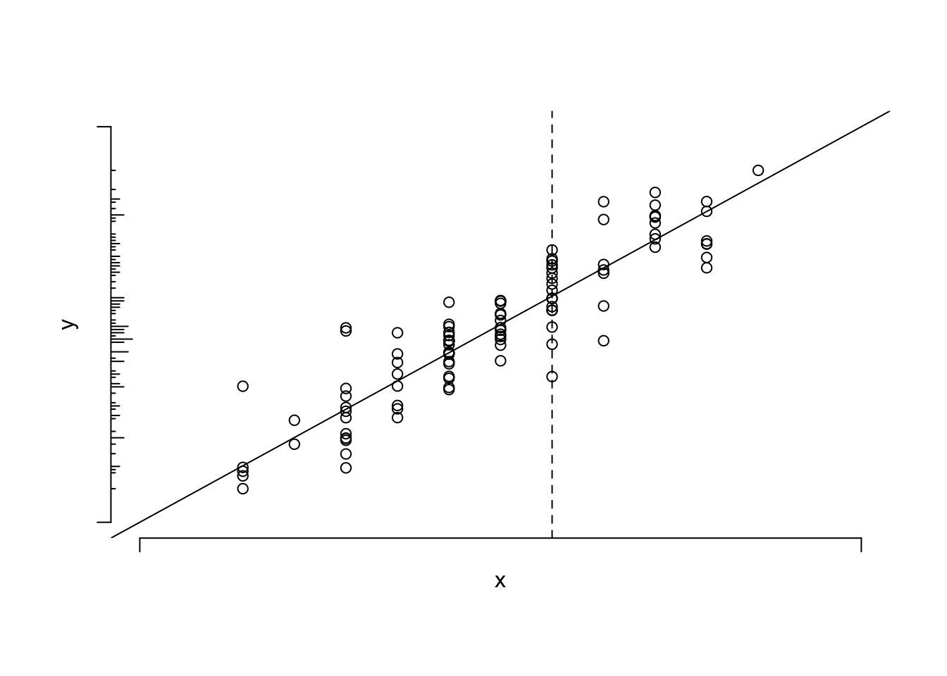
#| fig-cap: 'Data from a sample of $n=100$ points along with population linear regression line. The $x$ variable is discrete. The conditional distribution of $y | x$ can be thought of as a vertical slice at $x$. The unconditional distribution of $y$ is shown on the $y$-axis. To envision the conditional normal distributions assumed for the underlying population, think of a bell-shaped curve coming out of the page, with its base along one of the vertical lines of points. The equal variance assumption dictates that the series of Gaussian curves for all the different $x$s have equal variances.'
#| fig-scap: 'Sample of $n=100$ points with a linear regression line'
par(mgp=c(1,1,0))
n <- 100
set.seed(13)
x <- round(rnorm(n, .5, .25), 1)
y <- x + rnorm(n, 0, .1)
r <- c(-.2, 1.2)
plot(x, y, axes=FALSE, xlim=r, ylim=r, xlab=expression(x), ylab=expression(y))
axis(1, at=r, labels=FALSE)
axis(2, at=r, labels=FALSE)
abline(a=0,b=1)
histSpike(y, side=2, add=TRUE)
abline(v=.6, lty=2)
```
* $E(y|x)$ : population expected value or long-run average of $y$
conditioned on the value of $x$ <br>
Example: population average blood pressure for a 30-year old
* $\alpha$ : $y$-intercept
* $\beta$ : slope of $y$ on $x$ ($\frac{\Delta y}{\Delta x}$)
Simple linear regression is used when `r ipacue()`
* Only two variables are of interest
* One variable is a response and one a predictor
* No adjustment is needed for confounding or other between-subject
variation
* The investigator is interested in assessing the strength of the
relationship between $x$ and $y$ in real data units, or in
predicting $y$ from $x$
* A linear relationship is assumed (why assume this? why not use
nonparametric regression?)
* Not when one only needs to test for association (use Spearman's
$\rho$ rank correlation) or estimate a correlation index
### Two Ways of Stating the Model
`r mrg(sound("reg-3"))`
`r ipacue()`
* $E(y|x) = \alpha + \beta x$
* $y = \alpha + \beta x + e$ <br>
$e$ is a random error (residual) representing variation between
subjects in $y$ even if $x$ is constant, e.g. variation in
blood pressure for patients of the same age
### Assumptions, If Inference Needed
`r ipacue()`
* Conditional on $x$, $y$ is normal with mean $\alpha + \beta x$
and constant variance $\sigma^2$, <b>or:</b>
* $e$ is normal with mean 0 and constant variance $\sigma^2$
* $E(y|x) = E(\alpha + \beta x + e) = \alpha + \beta x + E(e)$, <br>
$E(e) = 0$.
* Observations are independent
### How Can $\alpha$ and $\beta$ be Estimated?
`r ipacue()`
* Need a criterion for what are good estimates
* <b>One</b> criterion is to choose values of the two parameters
that minimize the sum of squared errors in predicting individual
subject responses
* Let $a, b$ be guesses for $\alpha, \beta$
* Sample of size $n: (x_{1}, y_{1}), (x_{2}, y_{2}), \ldots,
(x_{n},y_{n})$
* $SSE = \sum_{i=1}^{n} (y_{i} - a - b x_{i})^2$
* Values that minimize $SSE$ are <em>least squares estimates</em>
* These are obtained from
`r ipacue()` $$\begin{array}{cc}
L_{xx} = \sum(x_{i}-\bar{x})^2 & L_{xy} = \sum(x_{i}-\bar{x})(y_{i}-\bar{y}) \\
\hat{\beta} = b = \frac{L_{xy}}{L_{xx}} & \hat{\alpha} = a =
\bar{y}- b \bar{x}
\end{array}$$
* Note: A term from $L_{xy}$ will be positive when $x$ and $y$ are
concordant in terms of both being above their means or both being
below their means.
* Least squares estimates are optimal if
1. the residuals truly come from a normal distribution
1. the residuals all have the same variance
1. the model is correctly specified, i.e., linearity holds
* Demonstration:
`r mrg(movie("https://youtu.be/4SPCQRCxuWI"))`
```{r lsdemo,eval=FALSE}
require(Hmisc)
getRs('demoLeastSquares.r')  # will load code into RStudio script editor
                             # click the Source button to run and follow
                             # instructions in console window
getRs('demoLeastSquares.r', put='source')   # if not using RStudio
```
### Inference about Parameters
`r mrg(sound("reg-4"))`<br>`r ipacue()`
* Estimated residual: $d = y - \hat{y}$
* $d$ large if line was not the proper fit to the data or if there
is large variability across subjects for the same $x$
* Beware of that many authors combine both components when using
the terms <em>goodness of fit</em> and <em>lack of fit</em>
* Might be better to think of lack of fit as being due to a
structural defect in the model (e.g., nonlinearity)
* $SST = \sum_{i=1}^{n} (y_{i} - \bar{y}) ^ {2}$ <br>
$SSR = \sum (\hat{y}_{i} - \bar{y}) ^ {2}$ <br>
$SSE = \sum (y_{i} - \hat{y}_{i}) ^ 2$ <br>
$SST = SSR + SSE$ <br>
$SSR = SST - SSE$
* $SS$ increases in proportion to $n$
* Mean squares: normalized for for d.f.: $\frac{SS}{d.f.(SS)}$
* $MSR = SSR / p$, $p$ = no. of parameters besides intercept
(here, 1) <br>
$MSE = SSE / (n - p - 1)$ (sample conditional variance of $y$)<br>
$MST = SST / (n - 1)$ (sample unconditional variance of $y$)
* Brief review of ordinary ANOVA (analysis of variance):
+ Generalizes 2-sample $t$-test to $> 2$ groups
+ $SSR$ is $SS$ between treatment means
+ $SSE$ is $SS$ within treatments, summed over treatments
* ANOVA Table for Regression `r ipacue()`
| Source | d.f. | $SS$ | $MS$ | $F$ |
|-----|-----|-----|-----|-----|
| Regression | $p$ | $SSR$ | $MSR = SSR/p$ | $MSR/MSE$ |
| Error | $n-p-1$ | $SSE$ | $MSE = SSE/(n-p-1)$ | |
| Total | $n-1$ | $SST$ | $MST = SST/(n-1)$ | |
* Statistical evidence for large values of $\beta$ can be
summarized by $F = \frac{MSR}{MSE}$
* Has $F$ distribution with $p$ and $n-p-1$ d.f.
* Large values $\rightarrow |\beta|$ large
* SST: how much subjects differ from each other -- proportional to sample variance of Y
* SSR: how much predictions for different subjects differ from each other (variation in Y explained by X)
* SSE: how much variation in Y cannot be explained by the model = sum of squared errors = total variation minus explained variation = SST - SSR
* Null model (only intercept): SSR = 0, SSE = SST
### Estimating $\sigma$, S.E. of $\hat{\beta}$; $t$-test
`r ipacue()`
* $s_{y\cdot x}^{2} = \hat{\sigma}^{2} = MSE = \widehat{Var}(y|x) =
\widehat{Var}(e)$
* $\widehat{se}(b) = s_{y\cdot x}/L_{xx}^\frac{1}{2}$
* $t = b / \widehat{se}(b), n-p-1$ d.f.
* $t^{2} \equiv F$ when $p=1$
* $t_{n-2} \equiv \sqrt{F_{1, n-2}}$
* $t$ identical to 2-sample $t$-test ($x$ has two values)
* If $x$ takes on only the values 0 and 1, $b$ equals ($\bar{y}$
when $x=1$) minus ($\bar{y}$ when $x=0$)
### Interval Estimation
`r mrg(sound("reg-5"))`<br>`r ipacue()`
* 2-sided $1-\alpha$ CI for $\beta$: $b \pm t_{n-2,1-\alpha/2}
\widehat{se}(b)$
* CI for <em>predictions</em> depend on what you want to predict
even though $\hat{y}$ estimates both $y$ ^[With a normal distribution, the least dangerous guess for an individual $y$ is the estimated mean of $y$.] and $E(y|x)$
* Notation for these two goals: $\hat{y}$ and $\hat{E}(y|x)$
+ Predicting $y$ with $\hat{y}$ : `r ipacue()` <br> $\widehat{s.e.}(\hat{y}) = s_{y \cdot x} \sqrt{1 + \frac{1}{n} + \frac{(x-\bar{x})^{2}}{L_{xx}}}$ <br><b>Note</b>: This s.e. $\rightarrow s_{y\cdot x}$ as $n \rightarrow \infty$
- As $n\rightarrow \infty$, $\widehat{s.e.}(\hat{y}) \rightarrow s_{y \cdot x}$ which is $> 0$
- Fits with thinking of a predicted individual value being the predicted mean plus a randomly chosen residual (the former has SD going to zero as $n \rightarrow \infty$ and the latter has SD of $s_{y \cdot x}$)
- This is a valid predicted individual value but not the lowest mean squared error prediction which would be just to predict at the middle (the mean)
+ Predicting $\hat{E}(y|x)$ with $\hat{y}$: `r ipacue()` <br>
$\widehat{s.e.}(\hat{E}(y|x)) = s_{y \cdot x} \sqrt{\frac{1}{n} +
\frac{(x-\bar{x})^{2}}{L_{xx}}}$ See footnote^[$n$ here is the grand total number of observations because we are borrowing information about neighboring $x$-points, i.e., using interpolation. If we didn't assume anything and just computed mean $y$ at each separate $x$, the standard error would instead by estimated by $s_{y\cdot x}\sqrt{\frac{1}{m}}$, where $m$ is the number of original observations with $x$ exactly equal to the $x$ for which we are obtaining the prediction. The latter s.e. is much larger than the one from the linear model.] <br>
<b>Note</b>: This s.e. shrinks to 0 as $n \rightarrow \infty$
* $1-\alpha$ 2-sided CI for either one: <br>
$\hat{y} \pm t_{n-p-1,1-\alpha/2}\widehat{s.e.}$
* Wide CI (large $\widehat{s.e.}$) due to:
+ small $n$
+ large $\sigma^2$
+ being far from the data center ($\bar{x}$)
* Example usages:
+ Is a child of age $x$ smaller than predicted for her age? <br>
Use $s.e.(\hat{y})$
+ What is the best estimate of the population mean blood pressure for
patients on treatment $A$? <br>
Use $s.e.(\hat{E}(y|x))$
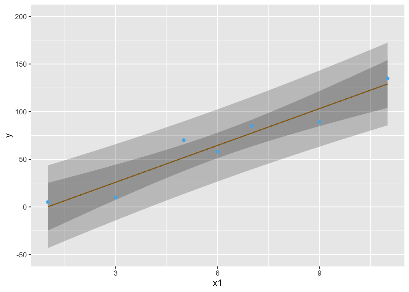
* Example pointwise 0.95 confidence bands: `r ipacue()` <br>
| $x$ | 1 | 3 | 5 | 6 | 7 | 9 | 11 |
|-----|-----|-----|-----|-----|-----|-----|-----|
| $y$:| 5 | 10 | 70 | 58 | 85 | 89 | 135 |
```{r both-type-cls}
#| label: fig-reg-both-type-cls
#| fig-cap: 'Pointwise 0.95 confidence intervals for $\hat{y}$ (wider bands) and $\hat{E}(y|x)$ (narrower bands).'
#| fig-scap: 'Two types of confidence bands'
require(rms)
x1 <- c( 1,  3,  5,  6,  7,  9,  11)
y  <- c( 5, 10, 70, 58, 85, 89, 135)
dd <- datadist(x1, n.unique=5); options(datadist='dd')
f <- ols(y ~ x1)
p1 <- Predict(f, x1=seq(1,11,length=100), conf.type='mean')
p2 <- Predict(f, x1=seq(1,11,length=100), conf.type='individual')
p <- rbind(Mean=p1, Individual=p2)
ggplot(p, legend.position='none') +
     geom_point(aes(x1, y), data=data.frame(x1, y, .set.=''))
```
### Assessing Goodness of Fit
`r mrg(sound("reg-6"), disc("reg-simple-gof"))`
Assumptions:
1. Linearity `r ipacue()`
1. $\sigma^2$ is constant, independent of $x$
1. Observations ($e$'s) are independent of each other
1. For proper statistical inference (CI, $P$-values), $e$ is normal, or equivalently, $y$ is normal conditional on $x$
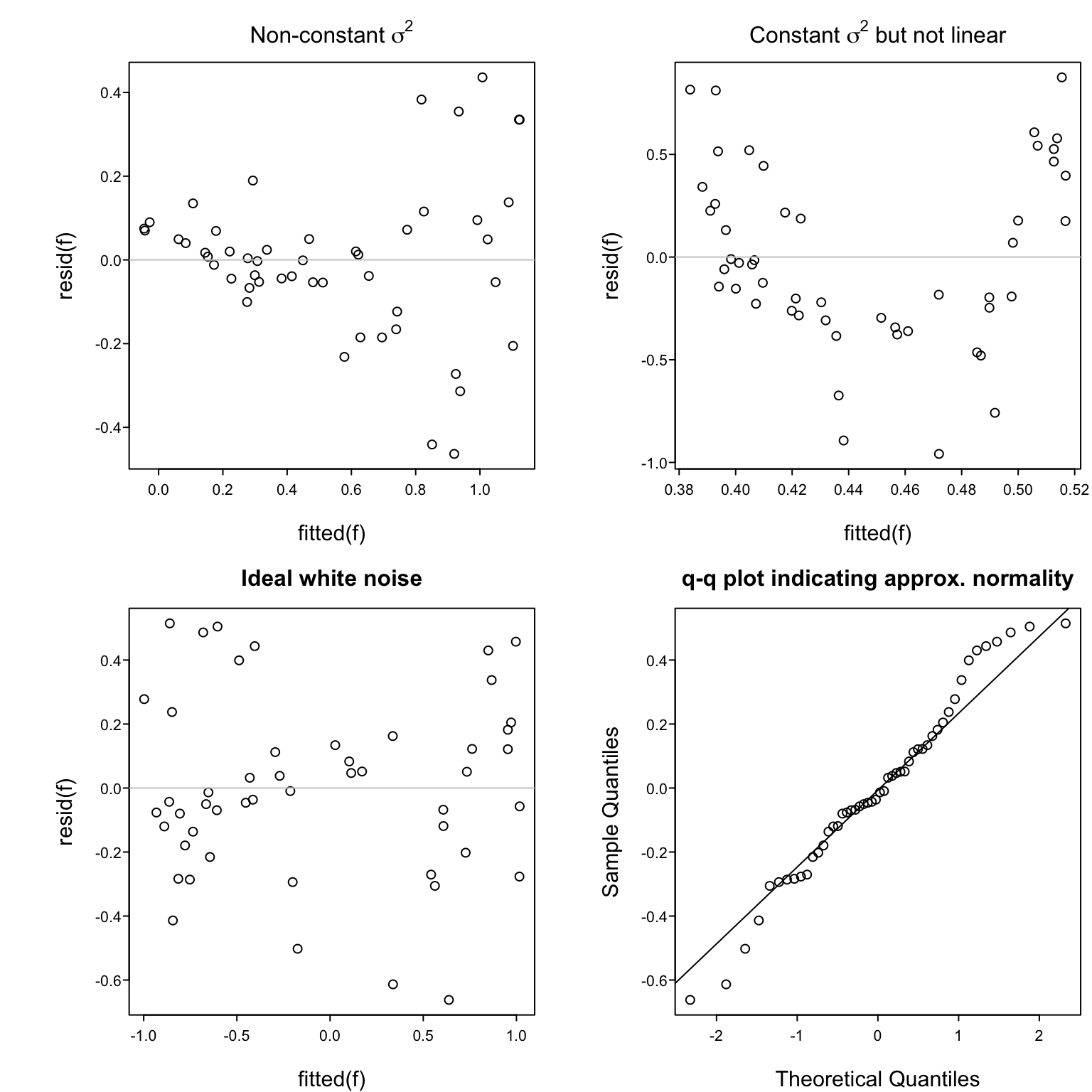
Verifying some of the assumptions: `r ipacue()`
* In a scattergram the spread of $y$ about the fitted line
should be constant as $x$ increases, and $y$ vs. $x$ should
appear linear
* Easier to see this with a plot of $\hat{d} = y - \hat{y}$ vs.\
$\hat{y}$
* In this plot there are no
systematic patterns (no trend in central tendency, no change
in spread of points with $x$)
* Trend in central tendency indicates failure of linearity
* <tt>qqnorm</tt> plot of $d$
<!--
#| fig-cap: 'Using residuals to check some of the assumptions of the simple linear regression model.'
#| fig-subcap:
#| - "Non-constant $\\sigma^2$, which might call for transforming $y$"
#| - "Constant $\\sigma^2$ but systemic failure of the linearity assumption"
#| - "Ideal situation of white noise (no trend, constant variance)"
#| - "$q-q$ plot demonstrating approximate normality of residuals, for a sample of size $n=50$. Horizontal reference lines are at zero, which is by definition the mean of all residuals."
#| layout-ncol: 2
#| fig-cap-location: bottom
-->
```{r exresid}
#| label: fig-reg-exresid
#| fig-cap: 'Using residuals to check some of the assumptions of the simple linear regression model.'
#| fig-width: 8
#| fig-height: 8
#| fig-scap: 'Four examples of residual plots'
spar(top=2, mfrow=c(2,2))
# Fit a model where x and y should have been log transformed
n <- 50
set.seed(2)
res <- rnorm(n, sd=.25)
x <- runif(n)
y <- exp(log(x) + res)
f <- ols(y ~ x)
plot(fitted(f), resid(f),
  main=expression(paste('Non-constant ', sigma^2)))
rl <- function() abline(h=0, col=gray(0.8))
rl()
# Fit a linear model that should have been quadratic
x <- runif(n, -1, 1)
y <- x ^ 2 + res
f <- ols(y ~ x)
plot(fitted(f), resid(f),
  main=expression(paste('Constant ', sigma^2, ' but not linear')))
rl()
# Fit a correctly assumed linear model
y <- x + res
f <- ols(y ~ x)
plot(fitted(f), resid(f), main='Ideal white noise')
rl()
# Q-Q plot to check normality of residuals
qqnorm(resid(f), main='q-q plot indicating approx. normality')
qqline(resid(f))
```
### Summary: Useful Equations for Linear Regression
Simple linear regression: one predictor ($p=1$): <br>
Model: $E(y|x) = \alpha + \beta x$ <br>
$E(y)$ = expectation or long--term average of $y|x$, $|$ = conditional on <br>
Alternate statement of model: $y = \alpha + \beta x + e,\quad e$
normal with mean zero for all $x$, $\quad var(e) = \sigma^{2} = var(y | x)$
Assumptions: `r ipacue()`
1. Linearity
1. $\sigma^2$ is constant, independent of $x$
1. Observations ($e$'s) are independent of each other
1. For proper statistical inference (CI, $P$--values), $e$ is
normal, or equivalently $y$ is normal conditional on $x$
Verifying some of the assumptions: `r ipacue()`
1. In a scattergram the spread of $y$ about the fitted line
should be constant as $x$ increases
1. In a residual plot ($d = y - \hat{y}$ vs. $x$) there are no
systematic patterns (no trend in central tendency, no change
in spread of points with $x$)
Sample of size $n: (x_{1}, y_{1}), (x_{2}, y_{2}), \ldots, (x_{n},y_{n})$ `r ipacue()`
$$\begin{array}{cc}
L_{xx} = \sum(x_{i}-\bar{x})^2 & L_{xy} = \sum(x_{i}-\bar{x})(y_{i}-\bar{y}) \\
\hat{\beta} = b = \frac{L_{xy}}{L_{xx}} & \hat{\alpha} = a = \bar{y}- b \bar{x} \\
\hat{y} = a + bx = \hat{E}(y | x) & \textrm{estimate of~} E(y|x) =
\textrm{~estimate of y} \\
SST = \sum(y_{i} - \bar{y})^{2} & MST = \frac{SST}{n-1} = s_{y}^{2} \\
SSR = \sum(\hat{y}_{i} - \bar{y})^{2} & MSR = \frac{SSR}{p} \\
SSE = \sum(y_{i} - \hat{y_{i}})^{2} & MSE = \frac{SSE}{n-p-1} =
s_{y\cdot x}^{2} \\
SST = SSR + SSE & F = \frac{MSR}{MSE} =
\frac{R^{2}/p}{(1 - R^{2})/(n-p-1)} \sim F_{p,n-p-1} \\
R^{2} = \frac{SSR}{SST} & \frac{SSR}{MSE} \dot{\sim} \chi^{2}_{p} \\
(p=1) ~~ \widehat{s.e.}(b) = \frac{s_{y \cdot x}}{\sqrt{L_{xx}}} &
t = \frac{b}{\widehat{s.e.}(b)} \sim t_{n-p-1} \\
1-\alpha \,\text{two-sided CI for}\, \beta & b \pm
t_{n-p-1,1-\alpha/2}\widehat{s.e.}(b) \\
(p=1) ~~ \widehat{s.e.}(\hat{y}) = s_{y \cdot x} \sqrt{1 + \frac{1}{n} +
\frac{(x-\bar{x})^{2}}{L_{xx}}} & \\
1-\alpha \,\text{two-sided CI for}\, y & \hat{y} \pm
t_{n-p-1,1-\alpha/2}\widehat{s.e.}(\hat{y}) \\
(p=1) ~~ \widehat{s.e.}(\hat{E}(y|x)) = s_{y \cdot x} \sqrt{\frac{1}{n} +
\frac{(x-\bar{x})^{2}}{L_{xx}}} \\
1-\alpha \,\text{two-sided CI for}\, E(y|x) & \hat{y} \pm
t_{n-p-1,1-\alpha/2}\widehat{s.e.}(\hat{E}(y|x)) \\
\end{array}$$
Multiple linear regression: $p$ predictors, $p > 1$: <br>
Model: $E(y|x) = \alpha + \beta_{1} x_{1} + \beta_{2} x_{2} + \ldots +
\beta_{p} x_{p} + e$ <br>
Interpretation of $\beta_{j}$: effect on $y$ of increasing $x_{j}$ by
one unit, holding all other $x$'s constant <br>
Assumptions: same as for $p=1$ plus no interaction between the $x$'s
($x$'s act additively; effect of $x_{j}$ does not depend on the other $x$'s).
Verifying some of the assumptions: `r ipacue()`
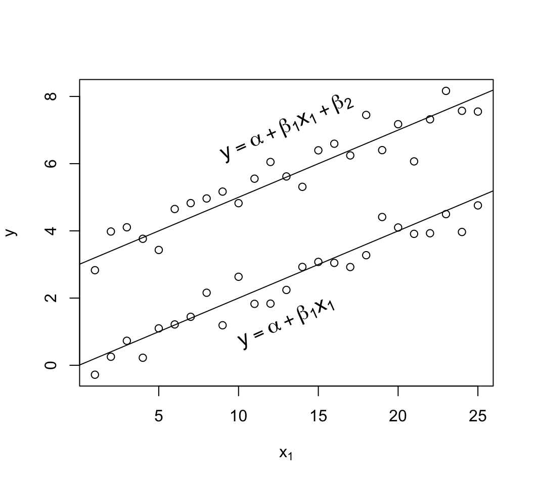
1. When $p=2$, $x_{1}$ is continuous, and $x_{2}$ is binary, the
pattern of $y$ vs. $x_{1}$, with points identified by
$x_{2}$, is two straight, parallel lines
1. In a residual plot ($d = y - \hat{y}$ vs. $\hat{y}$) there are no
systematic patterns (no trend in central tendency, no change
in spread of points with $\hat{y}$). The same is true if one
plots $d$ vs. any of the $x$'s.
1. Partial residual plots reveal the partial (adjusted)
relationship between a chosen $x_{j}$ and $y$, controlling for all
other $x_{i}, i \neq j$, without assuming linearity for $x_{j}$. In
these plots, the following quantities appear on the axes:
* <b>$y$ axis:</b> residuals from predicting $y$ from all predictors
except $x_j$
* <b>$x$ axis:</b> residuals from predicting $x_j$ from all
predictors except $x_{j}$ ($y$ is ignored)
When $p>1$, least squares estimates are obtained using more complex
formulas. But just as in the case with $p=1$, all of the coefficient
estimates are weighted combinations of the $y$'s, $\sum w_{i}y_{i}$
[when $p=1$, the $w_i$ for estimating $\beta$ are
$\frac{x_{i}-\bar{x}}{\sum(x_{i}-\bar{x})^{2}}$].
Hypothesis tests with $p>1$: `r ipacue()`
* Overall $F$ test tests $H_{0}: \beta_{1} = \beta_{2} = \ldots
\beta_{p} = 0$ vs. the althernative hypothesis that at least one of
the $\beta$'s $\neq 0$.
* To test whether an individual $\beta_{j}=0$ the simplest
approach is to compute the $t$ statistic, with $n-p-1$ d.f.
* Subsets of the $\beta$'s can be tested against zero if one
knows the standard errors of all of the estimated coefficients
and the correlations of each pair of estimates. The formulas
are daunting.
* To test whether a subset of the $\beta$'s are all zero, a good
approach is to compare the model containing all of the
predictors associated with the $\beta$'s of interest with a
sub--model containing only the predictors not being tested
(i.e., the predictors being adjusted for). This tests whether
the predictors of interest add response information to the
predictors being adjusted for. If the goal is to
test $H_{0}:\beta_{1}=\beta_{2}=\ldots=\beta_{q}=0$ regardless
of the values of $\beta_{q+1},\ldots,\beta_{p}$ (i.e.,
adjusting for $x_{q+1},\ldots,x_{p}$), fit the full model with
$p$ predictors, computing $SSE_{full}$ or $R^{2}_{full}$. Then
fit the sub--model omitting $x_{1},\ldots,x_{q}$ to obtain
$SSE_{reduced}$ or $R^{2}_{reduced}$. Then compute the
partial $F$ statistic
$F = \frac{(SSE_{reduced} - SSE_{full})/q}{SSE_{full}/(n-p-1)} = \frac{(R^{2}_{full} - R^{2}_{reduced})/q}{(1 - R^{2}_{full})/(n-p-1)} \sim F_{q,n-p-1}$
Note that $SSE_{reduced} - SSE_{full} = SSR_{full} - SSR_{reduced}$ .
Notes about distributions: `r ipacue()`
* If $t \sim t_{m}$ \, $t \dot{\sim}$ normal for large $m$ and $t^{2} \dot{\sim} \chi^{2}_{1}$, so ($\frac{b}{\widehat{s.e.}(b)})^{2} \dot{\sim} \chi^{2}_{1}$
* If $F \sim F_{m,n}, \quad m \times F \dot{\sim} \chi^{2}_{m}$ for large $n$
* If $F \sim F_{1,n}, \quad \sqrt{F} \sim t_{n}$
* If $t \sim t_{n}, \quad t^{2} \sim F_{1,n}$
* If $z \sim \mathrm{normal}, \quad z^{2} \sim \chi^{2}_{1}$
* $y \sim D$ means $y$ is distributed as the distribution $D$
* $y \dot{\sim} D$ means that $y$ is approximately distributed
as $D$ for large $n$
* $\hat{\theta}$ means an estimate of $\theta$
<!--
## Multivariable Modeling: General Issues
### Planning for Modeling
`r bookref("RMS", "1.4")`
* Response definition, follow-up, longitudinal vs. single time
* Variable definitions
* Observer variability
* Missing data
* Preference for continuous variables
* Subjects
* Sites
### Choice of the Model
`r bookref("RMS", "1.5")`
* In biostatistics and epidemiology we usually choose model
empirically
* Model must use data efficiently
* Should model overall structure (e.g., acute vs. chronic)
* Robust models are better
* Should have correct mathematical structure (e.g., constraints
on probabilities)
--->
## Proper Transformations and Percentiling
`r mrg(sound("reg-7"), disc("reg-percentiling"), bmovie(14), ddisc(14))`
* All parametric and semi-parametric regression models make
assumptions about the shape of the relationship between predictor
$X$ and response variable $Y$
* Many analysts assume linear relationships by default
* Regression splines (piecewise polynomials) are natural nonlinear
generalizations `r ipacue()`
* In epidemiology and public health many practitioners analyze
data using percentiling (e.g., of BMI against a random sample of the
population)
* This assumes that $X$ affects $Y$ though the population
distribution of $X$ (e.g., how many persons have BMI similar to a
subject) instead of through physics, physiology, or anatomy
* Also allows definitions to change as the population accommodates
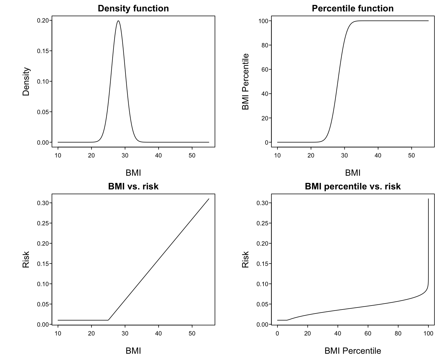
* Example: assume BMI is normal with mean 28 and SD 2 `r ipacue()`
* @fig-reg-bmi upper left panel shows this distribution
* Upper right: percentile of BMI vs. raw BMI
* Lower left: supposed relationship between BMI and disease risk
* Lower right: resulting relationship between BMI percentile and risk
All parametric regression models make assumptions about the form of
the relationship between the predictors $X$ and the response variable
$Y$. The typical default assumption is linearity in $X$ vs. some
transformation of $Y$ (e.g., log odds, log hazard or in ordinary
regression the identify function). Regression splines are one of the
best approaches for allowing for smooth, flexible regression function
shapes. Splines are described in detail in the <em>Regression Modeling Strategies</em> book and course notes.
Some researchers and government agencies get the idea that continuous
variables should be modeled through percentiling. This is a rather
bizarre way to attempt to account for shifts in the distribution of
the variable by age, race, sex, or geographic location. Percentiling
fails to recognize that the way that measurements affect subjects'
responses is through physics, physiology, anatomy, and other means.
Percentiling in effect states that how a variable affects the outcome
for a subject depends on how many other subjects there are like her.
When also percentiling variables (such as BMI) over time, the
measurement even changes its meaning over time. For example, updating
percentiles of BMI each year will keep the fraction of obese members
in the population constant even when obesity is truly on the rise.
Putting percentiles into a regression model assumes that the shape of
the $X-Y$ relationship is a very strange. As an example, suppose that
BMI has a normal distribution with mean 28 and standard deviation 2.
<!--
#| layout-nrow: 2
#| fig-width: 8
#| fig-height: 8
#| fig-subcap:
#| - "Density function for BMI"
#| - "Percentile function fo BMI"
#| - "BMI vs. risk"
#| - "BMI percentile vs. risk"
-->
```{r bmi}
#| label: fig-reg-bmi
#| fig-width: 8
#| fig-height: 6.5
#| fig-cap: 'Harm of percentiling BMI in a regression model'
spar(top=1, mfrow=c(2,2))
x <- seq(10, 55, length=200)
d <- dnorm(x, mean=28, sd=2)
plot(x, d, type='l', xlab='BMI', ylab='Density',
  main='Density function')
pctile <- 100*pnorm(x, mean=28, sd=2)
plot(x, pctile, type='l', xlab='BMI', ylab='BMI Percentile',
  main='Percentile function')
risk <- .01 + pmax(x - 25, 0)*.01
plot(x, risk, type='l', xlab='BMI', ylab='Risk',
  main='BMI vs. risk')
plot(pctile, risk, type='l', xlab='BMI Percentile', ylab='Risk',
  main='BMI percentile vs. risk')
```
Suppose that the true relationship between BMI and the risk of a
disease is given in the lower left panel. Then the relationship
between BMI percentile and risk must be that shown in the lower right
panel. To properly model that shape one must 'undo' the percentile
function then fit the result with a linear spline. Percentiling
creates unrealistic fits and results in more effort being spent if one
is to properly model the predictor. `r ipacue()`
* Worse still is to group $X$ into quintiles and use a linear
model in the quintile numbers
+ assumes are bizarre shape of relationship between $X$ and $Y$,
even if not noticing the discontinuities
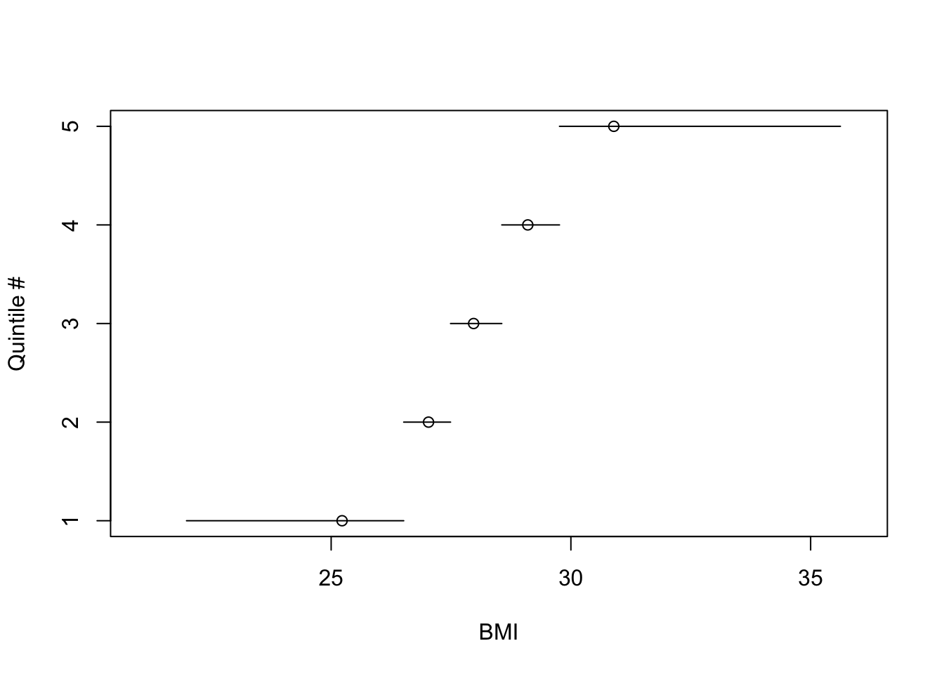
* @fig-reg-bmiq depicts quantile numbers vs. mean BMI
within each quintile. Outer quintiles:
+ have extremely skewed BMI distributions
+ are too heterogeneous to yield adequate BMI adjustment
(residual confounding)
* Easy to see that the transformation of BMI that yields quintile
numbers is discontinuous with variable step widths
In epidemiology a common practice is even more problematic. One often
`r ipacue()`
sees smoothly-acting continuous variables such as BMI broken into discontinuous quintile <em>groups</em>, the groups numbered from 1 to 5, and a linear regression of correlation fitted to the 1--5 variable
('test for trend'). This is not only hugely wasteful of information and power, but results in significant heterogeneity (especially in the outer quintiles) and
assumes a discontinuous effect on outcome that has an exceedingly
unusual shape when interpreted on the original BMI scale.
Taking the BMI distribution in @fig-reg-bmi consider what
this implies. We draw a random sample of size 500 from
the BMI distribution. @fig-reg-bmiq shows the
discontinuous relationship between BMI and quintile interval. The
location of the mean BMI within BMI quintile is a circle on each
horizontal line. One can see the asymmetry of the BMI distribution
in the outer quintiles, and that the meaning of inner quantiles is
fundamentally different than the meaning of the outer ones because of
the narrow range of BMI for inner quantile groups.
```{r bmiq}
#| label: fig-reg-bmiq
#| fig-cap: 'What are quintile numbers modeling?'
set.seed(1)
bmi  <- rnorm(500, mean=28, sd=2)
require(Hmisc)
bmiq <- cut2(bmi, g=5)
table(bmiq)
cuts <- cut2(bmi, g=5, onlycuts=TRUE)
cuts
bmim <- cut2(bmi, g=5, levels.mean=TRUE)
means <- as.numeric(levels(bmim))
plot(c(21, 36), c(1, 5), type='n', xlab='BMI', ylab='Quintile #')
for(i in 1 : 5) {
  lines(cuts[c(i, i+1)], c(i, i))
  points(means[i], i)
}
```
## Multiple Linear Regression
`r ems("11")`
`r mrg(abd("18"), bookref("RMS", "2.1-2.3"), disc("reg-mult"))`
### The Model and How Parameters are Estimated
`r mrg(sound("reg-8"))`
* $p$ independent variables $x_{1}, x_{2}, \ldots, x_{p}$
* Examples: multiple risk factors, treatment `r ipacue()`
plus patient descriptors when adjusting for non-randomized treatment
selection in an observational study; a set of controlled or
uncontrolled factors in an experimental study; indicators of
multiple experimental manipulations performed simultaneously
* Each variable has its own effect (slope) representing
<em>partial effects</em>: effect of increasing a variable by one unit,
holding all others constant
* Initially assume that the different variables act in an additive
fashion
* Assume the variables act linearly against $y$
* Model: $y = \alpha + \beta_{1}x_{1} + \beta_{2}x_{2} + \ldots + \beta_{p}x_{p} + e$ `r ipacue()`
* Or: $E(y|x) = \alpha + \beta_{1}x_{1} + \beta_{2}x_{2} + \ldots +
\beta_{p}x_{p}$
* For two $x$-variables: $y = \alpha + \beta_{1}x_{1} + \beta_{2}x_{2}$
* Estimated equation: $\hat{y} = a + b_{1}x_{1} + b_{2}x_{2}$
* Least squares criterion for fitting the model (estimating the
parameters): <br>
$SSE = \sum_{i=1}^{n} [y - (a + b_{1}x_{1} + b_{2}x_{2})]^2$
* Solve for $a, b_{1}, b_{2}$ to minimize $SSE$
* When $p>1$, least squares estimates require complex
formulas; still all of the coefficient estimates are weighted
combinations of the $y$'s, $\sum w_{i}y_{i}$^[When $p=1$, the $w_i$ for estimating $\beta$ are $\frac{x_{i}-\bar{x}}{\sum(x_{i}-\bar{x})^{2}}$].
### Interpretation of Parameters
`r mrg(sound("reg-9"))`<br>`r ipacue()`
* Regression coefficients are ($b$) are commonly called
<em>partial regression coefficients</em>: effects of each variable
holding all other variables in the model constant
* Examples of partial effects:
+ model containing $x_1$=age (years) and $x_2$=sex
(0=male 1=female) <br>
Coefficient of age ($\beta_1$) is the change in the mean of
$y$ for males when age increases by 1 year. It is also the change
in $y$ per unit increase in age for females. $\beta_2$ is the
female minus male mean difference in $y$ for two subjects of the
same age.
+ $E(y|x_{1},x_{2})=\alpha+\beta_{1}x_{1}$ for males,
$\alpha+\beta_{1}x_{1}+\beta_{2} =
(\alpha+\beta_{2})+\beta_{1}x_{1}$ for females [the sex effect is
a shift effect or change in $y$-intercept]
+ model with age and systolic blood pressure measured when the
study begins <br>
Coefficient of blood pressure is the change in mean $y$ when blood
pressure increases by 1mmHg for subjects of the same age
* What is meant by changing a variable? `r ipacue()`
+ We usually really mean a comparison of two subjects with
different blood pressures
+ Or we can envision what would be the expected response had
<em>this</em> subject's blood pressure been 1mmHg greater at the
outset^[This setup is the basis for randomized controlled trials and randomized animal experiments. Drug effects may be estimated with between-patient group differences under a statistical model.]
+ We are not speaking of longitudinal changes in a single
person's blood pressure
+ We can use subtraction to get the adjusted (partial) effect of
a variable, e.g.,
$$E(y|x_{1}=a+1,x_{2}=s)-E(y|x_{1}=a, x_{2}=s) =
\alpha + \beta_{1}(a+1) + \beta_{2}s -$$
$$(\alpha + \beta_{1}a + \beta_{2}s) = \beta_{1}$$
* Example: $\hat{y} = 37 + .01\times\textrm{weight} + 0.5\times\textrm{cigarettes smoked per day}$
+ .01 is the estimate of average increase $y$ across subjects when weight is increased by 1lb. if cigarette smoking is unchanged `r ipacue()`
+ 0.5 is the estimate of the average increase in $y$ across
subjects per additional cigarette smoked per day if weight does not
change
+ 37 is the estimated mean of $y$ for a subject of zero weight
who does not smoke
* Comparing regression coefficients:
+ Can't compare directly because of different units of
measurement. Coefficients in units of $\frac{y}{x}$.
+ Standardizing by standard deviations: not recommended. Standard
deviations are not magic summaries of scale and they give the wrong
answer when an $x$ is categorical (e.g., sex).
### Example: Estimation of Body Surface Area
`r mrg(sound("reg-9a"))`
DuBois & DuBois developed an equation in log height and log
weight in 1916 that is still used^[DuBois D, DuBois EF: A formula to estimate the approximate surface area if height and weight be known. <em>Arch Int Medicine</em> <b>17</b>(6):863-71, 1916.]. We use the main data they used
^[A Stata data file `dubois.dta` is available [here](https://hbiostat.org/data/repo/dubois.dta).].
```{r dubois}
require(rms)
d <- read.csv(textConnection(
'weight,height,bsa
24.2,110.3,8473
64.0,164.3,16720
64.1,178.0,18375
74.1,179.2,19000
93.0,149.7,18592
45.2,171.8,14901
32.7,141.5,11869
6.27,73.2,3699
57.6,164.8,16451
63.0,184.2,17981'))
d <- upData(d, labels=c(weight='Weight', height='Height',
                        bsa='Body Surface Area'),
            units=c(weight='kg', height='cm', bsa='cm^2'), print=FALSE)
d
# Create Stata file
getRs('r2stata.r', put='source')
dubois <- d
r2stata(dubois)
# Exclude subject measured using adhesive plaster method
d <- d[-7, ]
```
Fit a multiple regression model in the logs of all 3 variables `r ipacue()`
```{r dreg}
dd <- datadist(d); options(datadist='dd')
f <- ols(log10(bsa) ~ log10(weight) + log10(height), data=d)
f
```
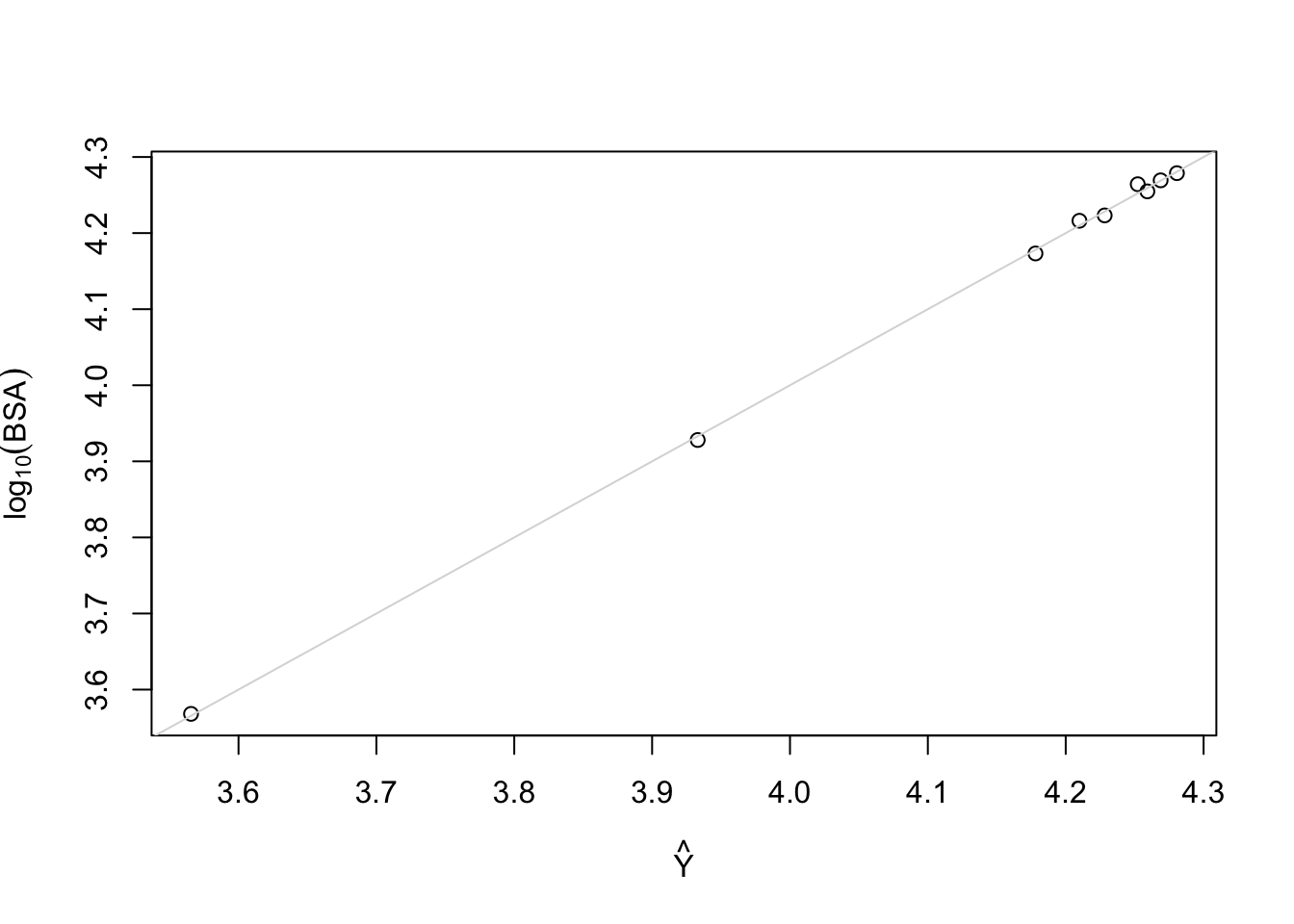
DuBois \& DuBois derived the equation log(bsa) = 1.8564 + 0.426
log(weight) + 0.725 log(height)
Plot predicted vs. observed
```{r dreg2}
plot(fitted(f), log10(d$bsa), xlab=expression(hat(Y)),
     ylab=expression(log[10](BSA))); abline(a=0, b=1, col=gray(.85))
```
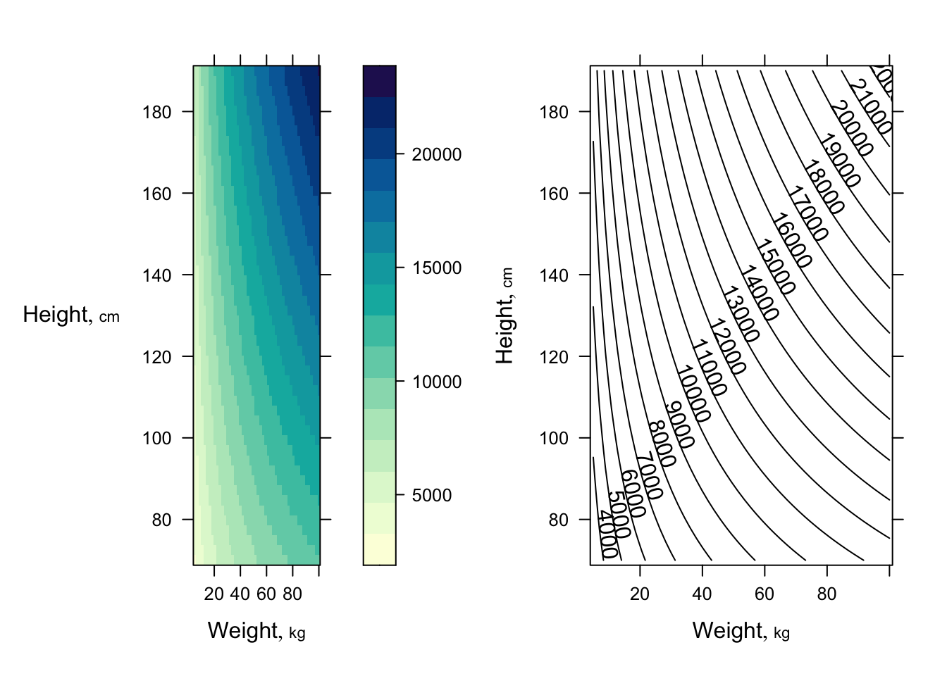
Get 3 types of plots to show fitted model `r ipacue()`
```{r dreg3,h=3.5,w=7.5}
require(lattice)  # provides contourplot, wireframe, ...
p <- Predict(f, weight=seq(5, 100, length=50),
             height=seq(70, 190, length=50), fun=function(z) 10 ^ z)
p1 <- bplot(p)
p2 <- bplot(p, lfun=contourplot, cuts=20)
arrGrob(p1, p2, ncol=2)
```
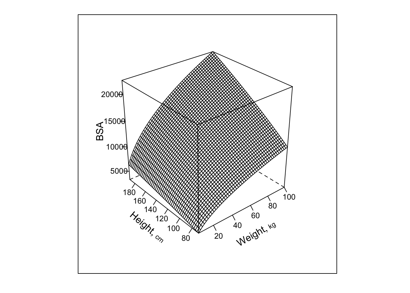
```{r dreg4,h=5,w=5}
bplot(p, lfun=wireframe, zlab='BSA')
```
Note: this plot would be a plane if all 3 variables were plotted on
the scale fitted in the regression ($\log_{10}$).
### What are Degrees of Freedom
`r mrg(sound("reg-10"))`<br>`r ipacue()`
* <b>For a model</b>: the total number of parameters not counting
intercept(s)
* <b>For a hypothesis test</b>: the number of parameters that are
hypothesized to equal specified constants. The constants specified
are usually zeros (for <em>null</em> hypotheses) but this is not
always the case. Some tests involve combinations of multiple
parameters but test this combination against a single constant; the
d.f. in this case is still one. Example: $H_{0}:
\beta_{3}=\beta_{4}$ is the same as $H_{0}:\beta_{3}-\beta_{4}=0$
and is a 1 d.f. test because it tests one parameter
($\beta_{3}-\beta_{4}$) against a constant ($0$).
These are <b>numerator d.f.</b> in the sense of the $F$-test in
multiple linear regression. The $F$-test also entails a second kind
of d.f., the <b>denominator</b> or <b>error</b> d.f., $n-p-1$,
where $p$ is the number of parameters aside from the intercept. The
error d.f. is the denominator of the estimator for $\sigma^2$ that is
used to unbias the estimator, penalizing for having estimated $p+1$
parameters by minimizing the sum of squared errors used to estimate
$\sigma^2$ itself. You can think of the error d.f. as the sample
size penalized for the number of parameters estimated, or as a measure
of the information base used to fit the model.
Other ways to express the d.f. for a hypothesis are: `r ipacue()`
* The number of opportunities you give associations to be present (relationships with $Y$ to be non-flat)
* The number of restrictions you place on parameters to make the null hypothesis of no association (flat relationships) hold
See also [hbiostat.org/glossary](https://hbiostat.org/glossary).
### Hypothesis Testing
`r ems("11.2")`<br>
`r mrg(disc("reg-mult-h0"))`
#### Testing Total Association (Global Null Hypotheses)
`r ipacue()`
* ANOVA table is same as before for general $p$
* $F_{p, n-p-1}$ tests $H_{0}:
\beta_{1}=\beta_{2}=\ldots=\beta_{p}=0$
* This is a test of <em>total association</em>, i.e., a test of
whether <em>any</em> of the predictors is associated with $y$
* To assess total association we accumulate partial effects of all
variables in the model <em>even though</em> we are testing if
<em>any</em> of the partial effects is nonzero
* $H_{a}:$ at least one of the $\beta$'s is non-zero.
<b>Note</b>: This does not mean that all of the $x$ variables are
associated with $y$.
* Weight and smoking example: $H_{0}$ tests the null hypothesis
that neither weight nor smoking is associated with $y$. $H_{a}$ is
that at least one of the two variables is associated with $y$. The
other may or may not have a non-zero $\beta$.
* Test of total association does not test whether cigarette
smoking is related to $y$ holding weight constant.
* $SSR$ can be called the model $SS$
#### Testing Partial Effects
`r mrg(sound("reg-11"), disc("reg-mult-h0-partial"))`
* $H_{0}: \beta_{1}=0$ is a test for the effect of $x_{1}$ on $y$
holding $x_{2}$ and any other $x$'s constant
* Note that $\beta_{2}$ is <em>not</em> part of the null or
alternative hypothesis; we assume that we have adjusted for
<em>whatever</em> effect $x_{2}$ has, <em>if any</em>
* One way to test $\beta_{1}$ is to use a $t$-test: $t_{n-p-1} = \frac{b_{1}}{\widehat{s.e.}(b_{1})}$ `r ipacue()`
* In multiple regression it is difficult to compute standard
errors so we use a computer
* These standard errors, like the one-variable case, decrease when
+ $n \uparrow$
+ variance of the variable being tested $\uparrow$
+ $\sigma^{2}$ (residual $y$-variance) $\downarrow$
* Another way to get partial tests: the $F$ test `r ipacue()`
+ Gives identical 2-tailed $P$-value to $t$ test when one $x$
being tested <br> $t^{2} \equiv$ partial $F$
+ Allows testing for $> 1$ variable
+ Example: is either systolic or diastolic blood pressure (or
both) associated with the time until a stroke, holding weight constant
* To get a partial $F$ define partial $SS$
* Partial $SS$ is the change in $SS$ when the variables
<b>being tested</b> are dropped from the model and the model is
re-fitted
* A general principle in regression models: a set of variables can
`r ipacue()`
be tested for their combined partial effects by removing that set of
variables from the model and measuring the harm ($\uparrow SSE$)
done to the model
* Let $full$ refer to computed values from the full model
including all variables; $reduced$ denotes a reduced model
containing only the adjustment variables and not the variables being
tested
* Dropping variables $\uparrow SSE, \downarrow SSR$ unless the
dropped variables had exactly zero slope estimates in the full model
(which never happens)
* $SSE_{reduced} - SSE_{full} = SSR_{full} - SSR_{reduced}$ <br>
Numerator of $F$ test can use either $SSE$ or $SSR$
* Form of partial $F$-test: change in $SS$ when dropping the
variables of interest divided by change in d.f., then divided by
$MSE$; <br>
$MSE$ is chosen as that which best estimates $\sigma^2$, namely the
$MSE$ from the full model
* Full model has $p$ slopes; suppose we want to test $q$ of the
slopes
`r ipacue()` $$\begin{array}{ccc}
F_{q, n-p-1} &=& \frac{(SSE_{reduced} - SSE_{full})/q}{MSE} \\
&=& \frac{(SSR_{full} - SSR_{reduced})/q}{MSE}
\end{array}$$
### Assessing Goodness of Fit
`r mrg(ems("12"), sound("reg-12"), disc("reg-mult-gof"))`<br>
`r ipacue()`
Assumptions:
* Linearity of each predictor against $y$ holding others constant
* $\sigma^2$ is constant, independent of $x$
* Observations ($e$'s) are independent of each other
* For proper statistical inference (CI, $P$-values), $e$ is
normal, or equivalently, $y$ is normal conditional on $x$
* $x$'s act additively; effect of $x_{j}$ does not depend on the
other $x$'s (<b>But</b> note that the $x$'s may be correlated with
each other without affecting what we are doing.)
Verifying some of the assumptions: `r ipacue()`
1. When $p=2$, $x_{1}$ is continuous, and $x_{2}$ is binary, the
pattern of $y$ vs. $x_{1}$, with points identified by
$x_{2}$, is two straight, parallel lines. $\beta_{2}$ is the
slope of $y$ vs. $x_{2}$ holding $x_{1}$ constant, which is
just the difference in means for $x_{2}=1$ vs. $x_{2}=0$ as
$\Delta x_{2}=1$ in this simple case.
```{r mult-reg-assume-twovar}
#| label: fig-reg-mult-reg-assume-twovar
#| fig-width: 5.5
#| fig-height: 5
#| fig-cap: 'Data satisfying all the assumptions of simple multiple linear regression in two predictors. Note equal spread of points around the population regression lines for the $x_{2}=1$ and $x_{2}=0$ groups (upper and lower lines, respectively) and the equal spread across $x_1$. The $x_{2}=1$ group has a new intercept, $\alpha+\beta_2$, as the $x_2$ effect is $\beta_2$. On the $y$ axis you can clearly see the difference between the two true population regression lines is $\beta_{2} = 3$.'
#| fig-scap: 'Assumptions for two predictors'
# Generate 25 observations for each group, with true beta1=.2, true beta2=3
d <- expand.grid(x1=1:25, x2=c(0, 1))
set.seed(3)
d$y <- with(d, .2*x1 + 3*x2 + rnorm(50, sd=.5))
with(d, plot(x1, y, xlab=expression(x[1]), ylab=expression(y)))
abline(a=0, b=.2)
abline(a=3, b=.2)
text(13, 1.3, expression(y==alpha + beta[1]*x[1]),           srt=24, cex=1.3)
text(13, 7.1, expression(y==alpha + beta[1]*x[1] + beta[2]), srt=24, cex=1.3)
```
1. In a residual plot ($d = y - \hat{y}$ vs. $\hat{y}$) there are no
systematic patterns (no trend in central tendency, no change
in spread of points with $\hat{y}$). The same is true if one
plots $d$ vs. any of the $x$'s (these are more stringent
assessments). If $x_{2}$ is binary box plots of $d$
stratified by $x_{2}$ are effective.
1. Partial residual plots reveal the partial (adjusted)
relationship between a chosen $x_{j}$ and $y$, controlling for all
other $x_{i}, i \neq j$, without assuming linearity for $x_{j}$. In
these plots, the following quantities appear on the axes:
* <b>$y$ axis:</b> residuals from predicting $y$ from all predictors
except $x_j$
* <b>$x$ axis:</b> residuals from predicting $x_j$ from all
predictors except $x_{j}$ ($y$ is ignored)
Partial residual plots ask how does what we can't predict about $y$
without knowing $x_j$ depend on what we can't predict about $x_j$ from
the other $x$'s.
## Multiple Regression with a Binary Predictor
`r mrg(disc("reg-xbinary"))`
### Indicator Variable for Two-Level Categorical Predictors
`r ipacue()`<br>
`r mrg(sound("reg-13"))`
* Categories of predictor: $A, B$ (for example)
* First category = reference cell, gets a zero
* Second category gets a 1.0
* Formal definition of indicator (dummy) variable: $x = [category=B]$ <br>
$[w]=1$ if $w$ is true, 0 otherwise
* $\alpha + \beta x = \alpha + \beta [category=B]$ = <br>
$\alpha$ for category $A$ subjects <br>
$\alpha + \beta$ for category $B$ subjects <br>
$\beta$ = mean difference ($B - A$)
### Two-Sample $t$-test vs. Simple Linear Regression
`r ipacue()`
* They are equivalent in every sense:
+ $P$-value
+ Estimates and C.L.s after rephrasing the model
+ Assumptions (equal variance assumption of two groups in
$t$-test is the same as constant variance of $y | x$ for every
$x$)
* $a = \bar{Y}_{A}$ <br>
$b = \bar{Y}_{B} - \bar{Y}_{A}$
* $\widehat{s.e.}(b) = \widehat{s.e.}(\bar{Y}_{B} - \bar{Y}_{A})$
### Analysis of Covariance
`r mrg(sound("reg-14"), disc("reg-ancova"))`
* Multiple regression can extend the $t$-test
+ More than 2 groups (multiple indicator variables can do multiple-group ANOVA) `r ipacue()`
+ Allow for categorical or continuous adjustment variables
(covariates, covariables)
* Example: lead exposure and neuro-psychological function (Rosner)
* Model: $MAXFWT = \alpha + \beta_{1} age + \beta_{2} sex + e$
* Rosner coded $sex=1, 2$ for male, female <br>
Does not affect interpretation of $\beta_2$ but makes interpretation
of $\alpha$ more tricky (mean $MAXFWT$ when $age=0$ and $sex=0$
which is impossible by this coding.
* Better coding would have been $sex=0, 1$ for male, female
+ $\alpha$ = mean $MAXFWT$ for a zero year-old male
+ $\beta_{1}$ = increase in mean $MAXFWT$ per 1-year increase in
$age$
+ $\beta_{2} =$ mean $MAXFWT$ for females minus mean $MAXFWT$ for
males, holding $age$ constant
* Suppose that we define an (arbitrary) `exposure` variable to `r ipacue()`
mean that the lead dose $\geq$ 40mg/100ml in either 1972 <b>or</b> 1973
* Model: $MAXFWT = \alpha + \beta_{1} exposure + \beta_{2} age +
\beta_{3} sex + e$ <br>
`exposure` = `TRUE` (1) for exposed, `FALSE` (0) for unexposed
* $\beta_{1}$ = mean $MAXFWT$ for exposed minus mean for
unexposed, holding $age$ and $sex$ constant
<!-- * Pay attention to Rosner's-->
<!-- \bi-->
<!-- * $t$ and $F$ statistics and what they test-->
<!-- * Figure 11.28 for checking for trend and equal variability of-->
<!-- residuals (don't worry about standardizing residuals)-->
<!-- \ei-->
## The Correlation Coefficient Revisited
`r mrg(sound("reg-15"), disc("reg-corr"))`
Pearson product-moment linear correlation coefficient:
`r ipacue()` $$\begin{array}{ccc}
r &=& \frac{L{xy}}{\sqrt{L_{xx}L_{yy}}} \\
&=& \frac{s_{xy}}{s_{x}s_{y}} \\
&=& b \sqrt{\frac{L_{xx}}{L_{yy}}}
\end{array}$$
* $r$ is unitless `r ipacue()`
* $r$ estimates the population correlation coefficient $\rho$ (not
to be confused with Spearman $\rho$ rank correlation coefficient)
* $-1 \leq r \leq 1$
* $r = -1$ : perfect negative correlation
* $r = 1$ : perfect positive correlation
* $r = 0$ : no correlation (no association)
* $t-test$ for $r$ is identical to $t$-test for $b$
* $r^2$ is the proportion of variation in $y$ explained by
conditioning on $x$
* $(n-2) \frac{r^{2}}{1-r^{2}} = F_{1,n-2} = \frac{MSR}{MSE}$
* For multiple regression in general we use $R^2$ to denote the `r ipacue()`
fraction of variation in $y$ explained jointly by all the $x$'s
(variation in $y$ explained by the whole model)
* $R^{2} = \frac{SSR}{SST} = 1 - \frac{SSE}{SST} = 1 -$ fraction of unexplained variation
* $R^{2}$ is called the <em>coefficient of determination</em>
* $R^2$ is between 0 and 1
+ 0 when $\hat{y}_{i} = \bar{y}$ for all $i$; $SSE=SST$
+ 1 when $\hat{y}_{i} = y_{i}$ for all $i$; SSE=0
* $R^{2} \equiv r^{2}$ in the one-predictor case
## Using Regression for ANOVA
`r ems("9")`<br>
`r mrg(abd("18.1"), disc("reg-anova"))`
### Indicator Variables
`r mrg(sound("reg-16"))`
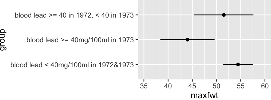
`Lead Exposure Group` (Rosner `lead` dataset): `r ipacue()`
* <b>control</b>: normal in both 1972 and 1973
* <b>currently exposed</b>: elevated serum lead level in 1973, normal in 1972
* <b>previously exposed</b>: elevated lead in 1972, normal in 1973
**NOTE**: This is not a very satisfactory way to analyze the two years' worth of lead exposure data, as we do not expect a discontinuous relationship between lead levels and neurological function. A continuous analysis was done in @sec-rmsintro-leadcontinuous.
`r ipacue()`
* Requires two indicator (dummy) variables (and 2 d.f.) to perfectly describe
3 categories
* $x_{1} = [$currently exposed$]$
* $x_{2} = [$previously exposed$]$
* Reference cell is control
* `lead` dataset `group` variable is set up this way already
* Model:
`r ipacue()` $$\begin{array}{ccc}
E(y|exposure) &=& \alpha + \beta_{1}x_{1} + \beta_{2}x_{2} \\
&=& \alpha, \textrm{controls} \\
&=& \alpha + \beta_{1}, \textrm{currently exposed} \\
&=& \alpha + \beta_{2}, \textrm{previously exposed}
\end{array}$$
`r ipacue()`
* <b>$\alpha$</b>: mean `maxfwt` for controls
* <b>$\beta_{1}$</b>: mean `maxfwt` for currently exposed minus mean
for controls
* <b>$\beta_{2}$</b>: mean `maxfwt` for previously exposed minus mean
for controls
* <b>$\beta_{2} - \beta_{1}$</b>: mean for previously exposed minus mean
for currently exposed
```{r olslead}
#| label: fig-reg-olslead
#| fig-cap: "Mean `maxfwt` by information-losing lead exposure groups"
#| fig-height: 1.75
#| fig-width: 4.75
getHdata(lead)
dd <- datadist(lead); options(datadist='dd')
f <- ols(maxfwt ~ group, data=lead)
f
ggplot(Predict(f))
summary(f)
```
* In general requires $k-1$ dummies to describe $k$ categories `r ipacue()`
* For testing or prediction, choice of reference cell is
irrelevant
* Does matter for interpreting individual coefficients
* Modern statistical programs automatically generate indicator
variables from categorical or character predictors^[In `R` indicators are generated automatically any time a `factor` or `category` variable is in the model.]
* In `R` never generate indicator variables yourself; just provide a `factor` or `character` predictor.
### Obtaining ANOVA with Multiple Regression
`r mrg(sound("reg-17"))`<br>`r ipacue()`
* Estimate $\alpha, \beta_{j}$ using standard least squares
* $F$-test for overall regression is exactly $F$ for ANOVA
* In ANOVA, $SSR$ is call sum of squares between treatments
* $SSE$ is called sum of squares within treatments
* Don't need to learn formulas specifically for ANOVA
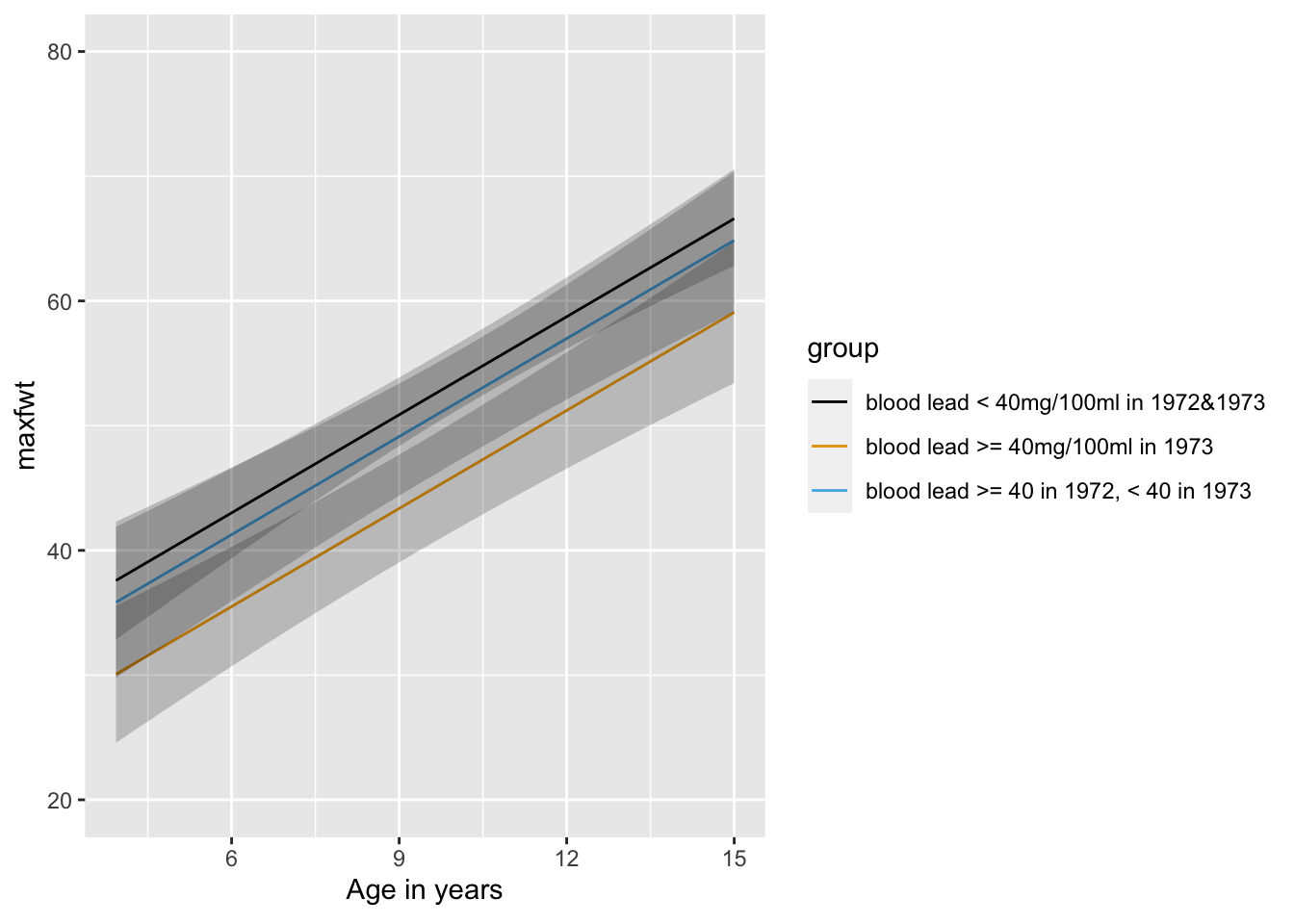
### One-Way Analysis of Covariance
`r ipacue()`
* Just add other variables (covariates) to the model
* Example: predictors age and treatment <br>
age is the covariate (adjustment variable)
* Global $F$ test tests the global null hypothesis that neither
age nor treatment is associated with response
* To test the adjusted treatment effect, use the partial $F$ test
for treatment based on the partial $SS$ for treatment adjusted for
age
* If treatment has only two categories, the partial $t$-test is an
easier way to get the age-adjusted treatment test
```{r leadgrage,w=6.5,h=3.5}
fa <- ols(maxfwt ~ age + group, data=lead)
fa
ggplot(Predict(fa, age, group))
summary(fa)
anova(fa)
anova(f) # reduced model (without age)
```
Subtract SSR or SSE from these two models to get the age effect with 1 d.f.
### Continuous Analysis of Lead Exposure
`r mrg(bmovie(15), ddisc(15))`
See @sec-rmsintro-leadcontinuous
### Two-Way ANOVA
`r mrg(sound("reg-18"))`<br>
`r ipacue()`
* Two categorical variables as predictors
* Each variable is expanded into indicator variables
* One of the predictor variables may not be time or episode within
subject; two-way ANOVA is often misused for analyzing repeated
measurements within subject
* Example: 3 diet groups (NOR, SV, LV) and 2 sex groups
* $E(y|diet,sex) = \alpha + \beta_{1}[SV] + \beta_{2}[LV] +
\beta_{3}[male]$
* Assumes effects of diet and sex are additive (separable) and not
synergistic
* $\beta_{1} = SV - NOR$ mean difference holding sex constant <br>
$\beta_{2} =$ LV - NOR mean difference holding sex constant <br>
$\beta_{3} =$ male - female effect holding diet constant
* Test of diet effect controlling for sex effect: <br>
$H_{0}:\beta_{1}=\beta_{2}=0$ <br>
$H_{a}: \beta_{1} \neq 0$ or $\beta_{2} \neq 0$
* This is a 2 d.f. partial $F$-test, best obtained by taking
difference in $SS$ between this full model and a model that excludes
all diet terms.
* Test for significant difference in mean $y$ for males vs.\
females, controlling for diet: <br>
$H_{0}: \beta_{3} = 0$
* For a model that has $m$ categorical predictors (only), none of
which interact, with numbers of categories given by $k_{1}, k_{2},
\ldots, k_{m}$, the total numerator regression d.f. is
$\sum_{i=1}^{m}(k_{i}-1)$
### Two-way ANOVA and Interaction
`r mrg(disc("reg-ia"))`
Example: sex (F,M) and treatment (A,B) <br>
Reference cells: F, A<br>
Model: <br>
$$\begin{array}{ccc}
E(y|sex,treatment) &=& \alpha + \beta_{1}[sex=M] \\
&+& \beta_{2}[treatment=B] + \beta_{3}[sex=M \cap treatment=B]
\end{array}$$
Note that $[sex=M \cap treatment=B] = [sex=M] \times
[treatment=B]$. `r ipacue()`
* <b>$\alpha$</b>: mean $y$ for female on treatment A (all variables at
reference values)
* <b>$\beta_{1}$</b>: mean $y$ for males minus mean for females, both on
treatment $A$ = sex effect holding treatment constant at $A$
* <b>$\beta_{2}$</b>: mean for female subjects on treatment $B$ minus
mean for females on treatment $A$ = treatment effect holding sex
constant at $female$
* <b>$\beta_{3}$</b>: $B-A$ treatment difference for males minus $B-A$
treatment difference for females <br>
Same as $M-F$ difference for treatment $B$ minus $M-F$ difference for
treatment $A$
In this setting think of interaction as a 'double difference'. To
understand the parameters: `r ipacue()`
| Group | $E(y|Group)$ |
|-----|-----|
| FA | $\alpha$ |
| MA | $\alpha + \beta_{1}$ |
| FB | $\alpha + \beta_{2}$ |
| MB | $\alpha + \beta_{1} + \beta_{2} + \beta_{3}$ |
Thus $MB - MA - [FB - FA] = \beta_{2} + \beta_{3} - \beta_{2} =
\beta_{3}$.
#### Heterogeneity of Treatment Effect
`r mrg(sound("reg-19"), disc("reg-hte"))`
Consider a Cox proportional hazards model for time
until first major cardiovascular event. The application is targeted
pharmacogenomics in acute coronary syndrome (the CURE study @par10eff). `r ipacue()`
* Subgroup analysis is virtually worthless for learning about differential treatment effects
* Instead a proper assessment of interaction must be used, with liberal adjustment for main effects
* An interaction effect is a double difference; for logistic and Cox models it is the ratio of ratios
* Interactions are harder to assess than main effects (wider confidence intervals, lower power)
* Carriers for loss-of-function CYP2C19 alleles: `r ipacue()` reduced conversion of clopidogrel to active metabolite
* Suggested that clop. less effective in reducing CV death, MI, stroke
* 12,562 (clop. HR 0.8); 5059 genotyped (clop. HR 0.7) `r ipacue()`
| | Carrier | | Non-Carrier |
|-----|-----|-----|-----|
| HR | 0.69 <small> (0.49, 0.98)</small> | | 0.72 <small> (0.59, 0.87)</small> |
| Ratio of HRs | | 0.96 <small> (0.64, 1.43)</small> | |
| | | <small> (P=0.8)</small> | |
* In the publication the needed ratio of hazard ratios was nowhere
to be found
* C.L. for ratio of hazard ratios shows that CYP2C19 variants may
plausibly be associated with a huge benefit or huge harm
* Point estimate is in the wrong direction
* Epidemiologic evidence points to a dominant effect of smoking in
this setting
+ Significant interaction between smoking status and clop. effect
+ Lack of evidence that clop. is effective in non-smokers
+ Gurbel, Nolin, Tantry, JAMA 2012:307:2495
<!-- http://jama.jamanetwork.com/article.aspx?articleID=1187938&utm_source=Silverchair%20Information%20Systems&utm_medium=email&utm_campaign=MASTER%3A_JAMA_Latest_Issue_TOC_Notification_06%2F20%2F2012-->
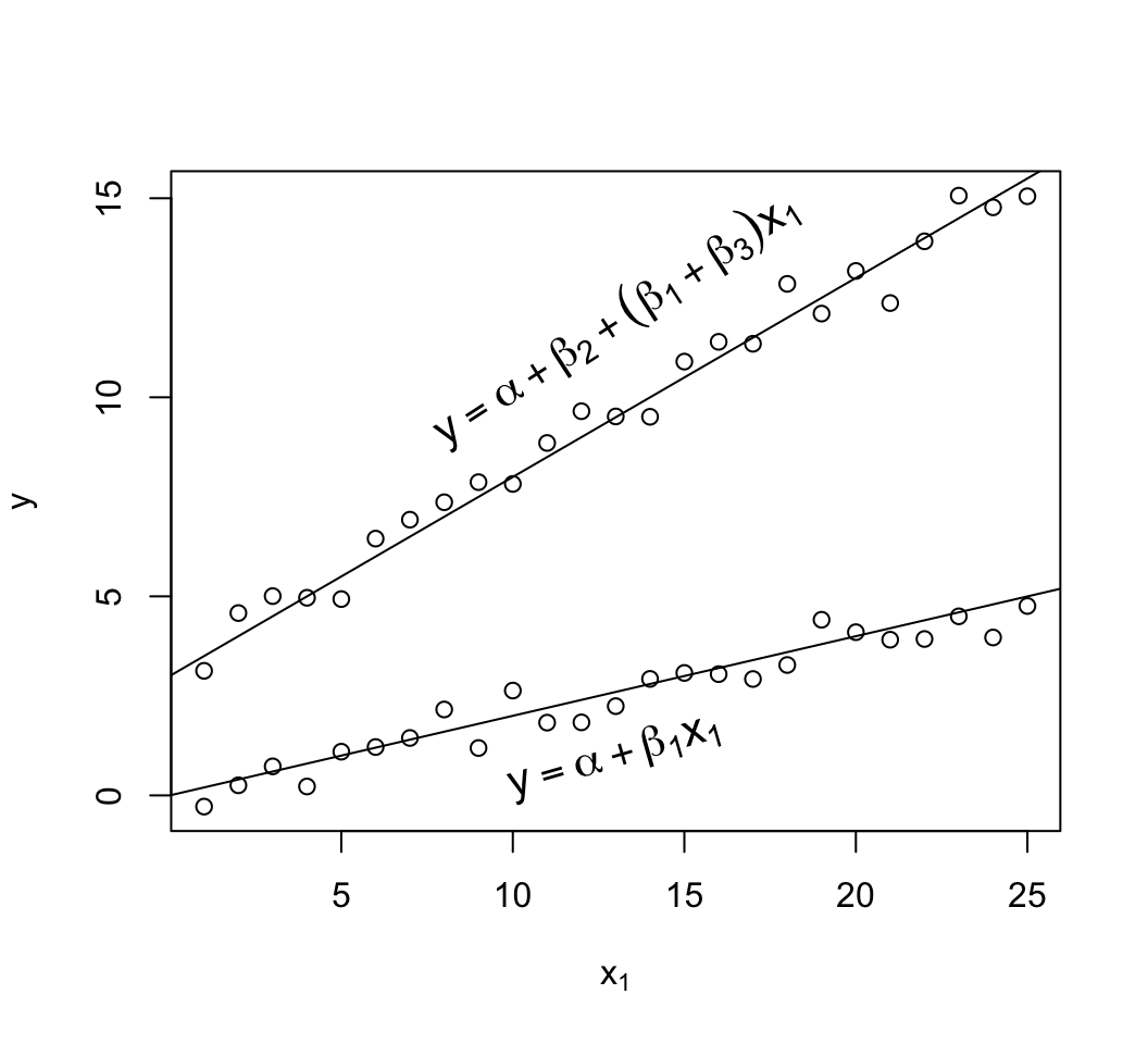
### Interaction Between Categorical and Continuous Variables
`r mrg(sound("reg-20"), disc("reg-ia-cc"))`
This is how one allows the slope of a predictor to vary by categories
of another variable. Example: separate slope for males and females: `r ipacue()`
$$\begin{array}{ccc}
E(y|x) &=& \alpha + \beta_{1}age + \beta_{2}[sex=m] \\
&+& \beta_{3}age\times [sex=m] \\
E(y|age, sex=f) &=& \alpha + \beta_{1}age \\
E(y|age, sex=m) &=& \alpha + \beta_{1}age + \beta_{2} + \beta_{3}age \\
&=& (\alpha + \beta_{2}) + (\beta_{1}+\beta_{3})age
\end{array}$$
* <b>$\alpha$</b>: mean $y$ for zero year-old female
* <b>$\beta_{1}$</b>: slope of age for females
* <b>$\beta_{2}$</b>: mean $y$ for males minus mean $y$ for females, for
zero year-olds
* <b>$\beta_{3}$</b>: increment in slope in going from females to males
```{r mult-reg-assume-twovar-ia}
#| fig-width: 5.5
#| fig-height: 5
#| fig-cap: 'Data exhibiting linearity in age but with interaction of age and sex. The $x_{2}=1$ group has a new intercept, $\alpha+\beta_2$ and its own slope $\beta_{1} + \beta_{3}$.'
#| fig-scap: 'Two predictors with interaction'
# Generate 25 observations for each group, with true beta1=.05, true beta2=3
d <- expand.grid(x1=1:25, x2=c(0, 1))
set.seed(3)
d$y <- with(d, 0.2*x1 + 3*x2 + 0.3*x1*x2 + rnorm(50, sd=.5))
with(d, plot(x1, y, xlab=expression(x[1]), ylab=expression(y)))
abline(a=0, b=.2)
abline(a=3, b=.5)
text(13, 1,  expression(y==alpha + beta[1]*x[1]), srt=16, cex=1.3)
text(13, 12, expression(y==alpha + beta[2] + (beta[1] + beta[3])*x[1]),
     srt=33, cex=1.3)
```
## Internal vs. External Model Validation <a name="reg-val"></a>
`r mrg(sound("reg-21"), disc("reg-val"), blog("split-val"))`
`r quoteit('External validation or validation on a holdout sample, when the predictive method was developed using feature selection, model selection, or machine learning, produces a non-unique <em>example</em> validation of a non-unique <em>example</em> model.', 'FE Harrell, 2015')`
`r ipacue()`
* Many researchers assume that 'external' validation of model
predictions is the only way to have confidence in predictions
* External validation may take years and may be low precision
(wide confidence intervals for accuracy estimates)
* Splitting one data sequence to create a holdout sample is
<em>internal</em> validation, not <em>external</em>, and resampling
procedures using all available data are almost always better
* External validation by splitting in time or place loses
opportunity for modeling secular and geographic trends, and often
results in failure to validate when in fact there are interesting
group differences or time trends that could have easily been modeled
* One should use all data available at analysis time `r ipacue()`
* External validation is left for newly collected data not
available at publication time
* Rigorous internal validation should be done first
+ 'optimism' bootstrap generally has lowest mean squared error
of accuracy estimates
+ boostrap estimates the likely future performance of model
developed on whole dataset
+ all analytical steps using $Y$ must be repeated for each of
approx. 300-400 bootstrap repetitions
+ when empirical feature selection is part of the process, the bootstrap
reveals the true volatility in the list of selected predictors
* Many data splitting or external validations are unreliable `r ipacue()`
(example: volatility of splitting 17,000 ICU patients with high
mortality, resulting in multiple splits giving different models and
different performance in holdout samples)
There are subtleties in what holdout sample validation actually means,
depending on how he predictive model is fitted: `r ipacue()`
* When the model's form is fully pre-specified, the external
validation validates that model and its estimated coefficients
* When the model is derived using feature selection or machine
learning methods, the holdout sample validation is not 'honest'' in
a certain sense:
+ data are incapable of informing the researcher what the
'right' predictors and the 'right' model are
+ the process doesn't recognize that the model being validated
is nothing more than an 'example' model
* Resampling for rigorous internal validation validates the `r ipacue()`
<em>process</em> used to derive the 'final' model
+ as a byproduct estimates the likely future performance of that model
+ while reporting volatility instead of hiding it
Model validation is a very important and complex topic that is covered
in detail in the two books mentioned below. One of the most
difficult to understand elements of validation is what is, and when to
use, external validation. Some researchers have published predictive
tools with no validation at all while other researchers falsely
believe that 'external' validation is the only valid approach to
having confidence in predictions. Frank Harrell (author of
<em>Regression Modeling Strategies</em>) and Ewout Steyerberg
(author of <em>Clinical Prediction Models</em>)
have written the text below in an attempt to illuminate several issues.
There is much controversy about the need for, definition of, and
timing of external validation.
A prognostic model should be valid outside the specifics of the sample
where the model is developed. Ideally, a model is shown to predict
accurately across a wide range of settings (Justice et al, <em>Ann Int Med</em> 1999). Evidence of such external validity requires evaluation by
different research groups and may take several years. Researchers
frequently make the mistake of labeling data splitting from a single
sequence of patients as external validation when in fact this is a
particularly low-precision form of internal validation better done
using resampling (see below). On the other hand, external validation
carried out by splitting in time (temporal validation) or by place,
is better replaced by considering interactions in the full dataset. For
example, if a model developed on Canadians is found to be poorly
calibrated for Germans, it is far better to develop an international
model with country as one of the predictors. This implies that a
researcher with access to data is always better off to analyze and
publish a model developed on the full set. That leaves external
validation using (1) newly collected data, not available at the time
of development; and (2) other investigators, at other sites, having
access to other data. (2) has been promoted by Justice as the
strongest form of external validation. This phase is only relevant
once internal validity has been shown for the developed model. But
again, if such data were available at analysis time, those data are
too valuable not to use in model development.
Even in the small subset of studies comprising truly external
validations, it is a common misconception that the validation statistics
are precise. Many if not most external validations are unreliable due to
instability in the estimate of predictive accuracy. This instability
comes from two sources: the size of the validation sample, and the
constitution of the validation sample. The former is easy to
envision, while the latter is more subtle. In one example, Frank
Harrell analyzed 17,000 ICU patients with $\frac{1}{3}$ of patients dying,
splitting the dataset into two halves - a training sample and a
validation sample. He found that the validation c-index (ROC area)
changed substantially when the 17,000 patients were re-allocated at
random into a new training and test sample and the entire process
repeated. Thus it can take quite a large external sample to yield
reliable estimates and to "beat" strong internal validation using
resampling. Thus we feel there is great utility in using strong
internal validation.
At the time of model development, researchers should focus on showing
internal validity of the model they propose, i.e. validity of the
model for the setting that they consider. Estimates of model
performance are usually optimistic. The optimism can efficiently be
quantified by a resampling procedure called the bootstrap, and the
optimism can be subtracted out to obtain an unbiased estimate of
future performance of the model on the same types of patients. The
bootstrap, which enjoys a strong reputation in data analysis, entails
drawing patients from the development sample with replacement. It
allows one to estimate the likely future performance of a predictive
model without waiting for new data to perform a external validation
study. It is important that the bootstrap model validation be done
rigorously. This means that all analytical steps that use the outcome
variable are repeated in each bootstrap sample. In this way, the
proper price is paid for any statistical assessments to determine the
final model, such as choosing variables and estimating regression
coefficients. When the resampling allows models and coefficients to
disagree with themselves over hundreds of resamples, the proper price
is paid for "data dredging", so that clinical utility (useful
predictive discrimination) is not claimed for what is in fact
overfitting (fitting "noise"). The bootstrap makes optimal use of the
available data: it uses all data to develop the model and all data to
internally validate the model, detecting any overfitting. One can
call properly penalized bootstrapping rigorous or strong internal
validation.
To properly design or interpret a predictive model validation it is
important to take into account how the predictions were formed. There
are two overall classes of predictive approaches: `r ipacue()`
* formulating a pre-specified statistical model based on
understanding of the literature and subject matter and using the
data to fit the parameters of the model but not to select the
<em>form</em> of the model or the features to use as predictors
* using the data to screen candidate predictive features or to
choose the form the predictions take. Examples of this class
include univariable feature screening, stepwise regression, and
machine learning algorithms.
External holdout sample validation may seem to be appropriate for the
second class but actually it is not 'honest' in the following
sense. The data are incapable of informing the researcher of what are
the 'right' predictors. This is even more true when candidate
predictors are correlated, creating competition among predictors and
arbitrary selections from these co-linear candidates. A predictive
rule derived from the second class of approaches is merely an
<em>example</em> of a predictive model. The only way for an analyst to
understand this point is to use resampling (bootstrap or
cross-validation) whereby predictive models (or machine learning
structures) are repeatedly derived from scratch and the volatility (and
difficulty of the task) are exposed.
So what goes in in the training and validation processes depends on
the class of predictive methods used: `r ipacue()`
* When the model is pre-specified except for the regression
coefficients that need to be estimated, rigorous resampling
validation validates the fit of <em>the</em> model and so does holdout
sample validation.
* When the model structure was not pre-specified but model/feature
selection was done, resampling validation validates the
<em>process</em> used to derive the 'final' model and as a
by-product estimates the likely future performance of this model
while documenting to the researcher that there is usually great
instability in the form of this model. It is imperative that the
analyst repeat <em>all</em> feature selection or model selection steps
afresh for each resample and displays the variation of features /
models selected across the resamples. For the bootstrap this
usually involves 300 or more resamples, and for cross-validation 50
or more repeats of 10-fold cross-validation. The 'final' model
should be described as an example of an entire array of models, and
the likely future performance of this example model is estimated
from the resampling procedure just described. Resampling alerts the
analyst to arbitrariness and reduces the tendency to cherry
pick good validations when split-sample or external validation is used.
Thus in the case just described where a statistical model is not fully
pre-specified, pretending to 'freeze' the 'final' result and
validating it on a holdout sample is problematic. The resulting
validation, far from being a validation of 'the' model is just an
example validation of an example model. On the other hand, rigorous
validation using resampling validates the process used to derive the
final predictive instrument, while still providing a good estimate of
the likely future predictive accuracy of that instrument.
### Summary: Choosing Internal vs. External Validation <a name="reg-choose-val"></a>
Recall that strong internal validation uses the bootstrap in a way
that repeats all modeling steps (feature/variable selection, transformation
selection, parameter estimation, etc.) that utilized the outcome
variable $Y$.
Use strong internal validation if `r ipacue()`
* the model is not pre-specified. If any feature selection
utilizing $Y$ was done, the set of features selected will be
unstable, so an external validation would just validate an ``example
model.'' On the other hand, a strong internal validation validates
the model development <em>process</em> and fully documents the
volatility of feature selection.
* the data come from multiple locations or times and you want to
understand time trends in $Y$, or geographic differences
* the size of the potential external validation sample and the
size of the training sample are not both very large
Use external validation if `r ipacue()`
* measurement platforms vary (e.g., genotyping or blood analysis
equipment) and you want to validate the generalizability of a model
developed on your platform
* both the training data and the test datasets are very large
(e.g., the training data contains more than 15 events per
<b>candidate</b> predictor and the test data has at least 200-400 events)
* the dataset to be used for the external validation was not
available when the model was developed and internally validated
* you don't trust the model developers to honestly perform a
strong internal validation
## Other Resources
`r ipacue()`
* [Prediction Research Manual](http://www.cecilejanssens.org/wp-content/uploads/2018/01/PredictionManual2.0.pdf) by Cecile Janssens and Forike Martens
* Steyerberg paper on the waste by data splitting: @ste18val.
## Study Questions
**Section 10.1**
1. What are some problems with matching as an adjustment strategy?
**Section 10.2-10.3**
1. Do we need the $t$-test, Wilcoxon test, and log-rank test?
1. Why is a statistical model required for estimating the effect of going from a systolic blood pressure of 120mmHg to one of 140mmHg?
**Section 10.4**
1. For a continuous response variable Y why are we often interested in estimating the long-term average and not an individual subject response?
1. What is an indication for a strong predictive model, thinking about SSR?
1. Why does the standard error for a predicted individual Y value almost never approach zero?
1. If you knew that the relationship between x and y is linear, what would be the best distribution of x for estimating the linear regression equation and for hypothesis testing?
1. If you did not know anything about the shape of the x-y relationship and wanted to model this smooth relationship, what would be the best study design?
**Section 10.5**
1. What are the central problems in percentiling variables?
**Section 10.6**
1. What essentially means the same whether discussing single-variable vs. multivariable regression?
1. Are model and hypothesis test d.f. most related to numerator d.f. or denominator d.f.?
1. Does rejecting the global test of no association imply that all the predictors are associated with Y?
1. What are two principal ways we test whether one or more predictors are associated with Y after adjusting for other variables?
**Section 10.7**
1. A linear model with a single binary predictor is equivalent to what?
2. Why is added more variables and doing ANCOVA better than this?
**Section 10.10**
1. A researcher wants to analyze the effect of race (4 levels) and sex on Y and wants to allow for race x sex interaction. How many model d.f. are there?
1. Why is heterogeneity of treatment effect difficult to demonstrate?
**Section 10.11**
1. Under what condition is it simple to understand what external validation is validating?
1. When is external validation a good idea?
```{r echo=FALSE}
saveCap('10')
```