9  Introduction to the R rms Package: The Linear Model

Some of the purposes of the rms package are toA

• make everyday statistical modeling easier to do
• make modern statistical methods easy to incorporate into everyday work
• make it easy to use the bootstrap to validate models
• provide “model presentation graphics”

9.1 Formula Language and Fitting Function

• Statistical formula in R: B

y ~ x1 + x2 + x3

y is modeled as \(\alpha + \beta_{1}x_{1} + \beta_{2}x_{2} + \beta_{3} x_{3}\)

• y is the dependent variable/response/outcome, x’s are predictors (independent variables)
• The formula is the first argument to a fitting function (just as it is the first argument to a trellis graphics function)
• rms (regression modeling strategies) package Harrell (2020) makes many aspects of regression modeling and graphical display of model results easier to do
• rms does a lot of bookkeeping to remember details about the design matrix for the model and to use these details in making automatic hypothesis tests, estimates, and plots. The design matrix is the matrix of independent variables after coding them numerically and adding nonlinear and product terms if needed.
• rms package fitting function for ordinary least squares regression (what is often called the linear model or multiple linear regression): ols
• Example: C

f <- ols(y ~ age + sys.bp, data=mydata)

• age and sys.bp are the two predictors (independent variables) assumed to have linear and additive effects (do not interact or have synergism)
• mydata is an R data frame containing at least three columns for the model’s variables
• f (the fit object) is an R list object, containing coefficients, variances, and many other quantities
• Below, the fit object will be f throughout. In practice, use any legal R name, e.g. fit.full.model

9.2 Operating on the Fit Object

D

• Regression coefficient estimates may be obtained by any of the methods listed below

f$coefficients
f$coef          # abbreviation
coef(f)         # use the coef extractor function
coef(f)[1]      # get intercept
f$coef[2]       # get 2nd coefficient (1st slope)
f$coef['age']   # get coefficient of age
coef(f)['age']  # ditto

• But often we use methods which do something more interesting with the model fit.
  • print(f): print coefficients, standard errors, \(t\)-test, other statistics; can also just type f to print
  • fitted(f): compute \(\hat{y}\)
  • predict(f, newdata): get predicted values, for subjects described in data frame newdata¹
  • r <- resid(f): compute the vector of \(n\) residuals (here, store it in r)
  • formula(f): print the regression formula fitted
  • anova(f): print ANOVA table for all total and partial effects
  • summary(f): print estimates partial effects using meaningful changes in predictors
  • Predict(f): compute predicted values varying a few predictors at a time (convenient for plotting)
  • ggplot(p): plot partial effects, with predictor ranging over the \(x\)-axis, where p is the result of Predict
  • g <- Function(f): create an R function that evaluates the analytic form of the fitted function
  • nomogram(f): draw a nomogram of the model

¹ You can get confidence limits for predicted means or predicted individual responses using the conf.int and conf.type arguments to predict. predict(f) without the newdata argument yields the same result as fitted(f).

Note: Some of othe functions can output html if options(prType='html') is set, as is done in this chapter. When using that facility you do not need to add results='asis' in the knitr chunk header as the html is sensed automatically.

9.3 The rms datadist Function

E

To use Predict, summary, or nomogram in the rms package, you need to let rms first compute summaries of the distributional characteristics of the predictors:

dd <- datadist(x1,x2,x3,...)   # generic form
dd <- datadist(age, sys.bp, sex)
dd <- datadist(mydataframe)    # for a whole data frame
options(datadist='dd')         # let rms know where to find

Note that the name dd can be any name you choose as long as you use the same name in quotes to options that you specify (unquoted) to the left of <- datadist(...). It is best to invoke datadist early in your program before fitting any models. That way the datadist information is stored in the fit object so the model is self-contained. That allows you to make plots in later sessions without worrying about datadist. datadist must be re-run if you add a new predictor or recode an old one. You can update it using for example

dd <- datadist(dd, cholesterol, height)
# Adds or replaces cholesterol, height summary stats in dd

9.4 Short Example

F

² maxfwt might be better analyzed as an ordinal variable but as will be seen by residual plots it is also reasonably considered to be continuous and to satisfy ordinary regression assumptions.

Consider the lead exposure dataset from B. Rosner Fundamentals of Biostatistics and originally from Landrigan PJ et al, Lancet 1:708-715, March 29, 1975. The study was of psychological and neurologic well-being of children who lived near a lead smelting plant. The primary outcome measures are the Wechsler full-scale IQ score (iqf) and the finger-wrist tapping score maxfwt. The dataset is available at hbiostat.org/data and can be automatically downloaded and load()’d into R using the Hmisc package getHdata function. For now we just analyze lead exposure levels in 1972 and 1973, age, and maxfwt².

G Commands listed in previous sections were not actually executed because their chunk headers contained eval=FALSE.

# For an Rmarkdown version of similar analyses see
# https://github.com/harrelfe/rscripts/raw/master/lead-ols.md
require(rms)    # also loads the Hmisc package
getHdata(lead)
# Subset variables just so contents() and describe() output is short
# Override units of measurement to make them legal R expressions
lead <- upData(lead,
               keep=c('ld72', 'ld73', 'age', 'maxfwt'),
               labels=c(age='Age'),
               units=c(age='years', ld72='mg/100*ml', ld73='mg/100*ml'))

Input object size:   53928 bytes;    39 variables    124 observations
Kept variables  ld72,ld73,age,maxfwt
New object size:    14096 bytes;    4 variables 124 observations

H

contents(lead)

---

Data frame:lead

124 observations and 4 variables, maximum # NAs:25  

---

Name	Labels	Units	Storage	NAs
age	Age	years	double	0
ld72	Blood Lead Levels, 1972	mg/100*ml	integer	0
ld73	Blood Lead Levels, 1973	mg/100*ml	integer	0
maxfwt	Maximum mean finger-wrist tapping score		integer	25

---

# load jQuery javascript dependencies for interactive sparklines
sparkline::sparkline(0)

print(describe(lead), 'continuous')

lead Descriptives
4 Continous Variables of 4 Variables, 124 Observations
Variable	Label	Units	n	Missing	Distinct	Info	Mean	Gini |Δ|		Quantiles .05 .10 .25 .50 .75 .90 .95
age	Age	years	124	0	73	1.000	8.935	4.074		3.929 4.333 6.167 8.375 12.021 14.000 15.000
ld72	Blood Lead Levels, 1972	mg/100*ml	124	0	47	0.999	36.16	17.23		18.00 21.00 27.00 34.00 43.00 57.00 61.85
ld73	Blood Lead Levels, 1973	mg/100*ml	124	0	37	0.998	31.71	11.06		18.15 21.00 24.00 30.50 37.00 47.00 50.85
maxfwt	Maximum mean finger-wrist tapping score		99	25	40	0.998	51.96	13.8		33.2 38.0 46.0 52.0 59.0 65.0 72.2

I

dd <- datadist(lead); options(datadist='dd')
dd    # show what datadist computed 

                      age  ld72  ld73 maxfwt
Low:effect       6.166667 27.00 24.00   46.0
Adjust to        8.375000 34.00 30.50   52.0
High:effect     12.020833 43.00 37.00   59.0
Low:prediction   3.929167 18.00 18.15   33.2
High:prediction 15.000000 61.85 50.85   72.2
Low              3.750000  1.00 15.00   13.0
High            15.916667 99.00 58.00   84.0

# Fit an ordinary linear regression model with 3 predictors assumed linear
f <- ols(maxfwt ~ age + ld72 + ld73, data=lead)

J

f         # same as print(f)

Linear Regression Model

ols(formula = maxfwt ~ age + ld72 + ld73, data = lead)

Frequencies of Missing Values Due to Each Variable

maxfwt    age   ld72   ld73 
    25      0      0      0 

	Model Likelihood Ratio Test	Discrimination Indexes
Obs 99	LR χ2 62.25	R2 0.467
σ 9.5221	d.f. 3	R2adj 0.450
d.f. 95	Pr(>χ2) 0.0000	g 10.104

Residuals

     Min       1Q   Median       3Q      Max 
-33.9958  -4.9214   0.7596   5.1106  33.2590 

	β	S.E.	t	Pr(>|t|)
Intercept	34.1059	4.8438	7.04	<0.0001
age	2.6078	0.3231	8.07	<0.0001
ld72	-0.0246	0.0782	-0.31	0.7538
ld73	-0.2390	0.1325	-1.80	0.0744

K

coef(f)   # retrieve coefficients

 Intercept        age       ld72       ld73 
34.1058551  2.6078450 -0.0245978 -0.2389695 

specs(f, long=TRUE)   # show how parameters are assigned to predictors,

ols(formula = maxfwt ~ age + ld72 + ld73, data = lead)

     Units     Label                   Assumption Parameters d.f.
age  years     Age                     asis                  1   
ld72 mg/100*ml Blood Lead Levels, 1972 asis                  1   
ld73 mg/100*ml Blood Lead Levels, 1973 asis                  1   

                      age  ld72  ld73
Low:effect       6.166667 27.00 24.00
Adjust to        8.375000 34.00 30.50
High:effect     12.020833 43.00 37.00
Low:prediction   3.929167 18.00 18.15
High:prediction 15.000000 61.85 50.85
Low              3.750000  1.00 15.00
High            15.916667 99.00 58.00

                      # and predictor distribution summaries driving plots

L

g <- Function(f)  # create an R function that represents the fitted model
# Note that the default values for g's arguments are medians
g

function (age = 8.375, ld72 = 34, ld73 = 30.5) 
{
    34.105855 + 2.607845 * age - 0.024597799 * ld72 - 0.23896951 * 
        ld73
}
<environment: 0x12631b1c8>

# Estimate mean maxfwt at age 10, .1 quantiles of ld72, ld73 and .9 quantile of ld73
# keeping ld72 at .1 quantile
g(age=10, ld72=21, ld73=c(21, 47))  # more exposure in 1973 decreased y by 6

[1] 54.64939 48.43618

M

# Get the same estimates another way but also get std. errors 
predict(f, data.frame(age=10, ld72=21, ld73=c(21, 47)), se.fit=TRUE)

$linear.predictors
       1        2 
54.64939 48.43618 

$se.fit
       1        2 
1.391858 3.140361 

9.5 Operating on Residuals

N

Residuals may be summarized and plotted just like any raw data variable.

• To plot residuals vs. each predictor, and to make a q-q plot to check normality of residuals, use these examples:

spar(mfrow=c(2,2))   # spar is in qreport; 2x2 matrix of plots
r <- resid(f)
plot(fitted(f), r); abline(h=0)  # yhat vs. r
with(lead, plot(age,  r));    abline(h=0)
with(lead, plot(ld73, r));    abline(h=0)
qqnorm(r)           # linearity indicates normality
qqline(as.numeric(r))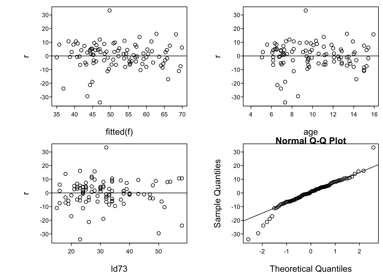

9.6 Plotting Partial Effects

O

• Predict and ggplot makes one plot for each predictor
• Predictor is on \(x\)-axis, \(\hat{y}\) on the \(y\)-axis
• Predictors not shown in plot are set to constants
  • median for continuous predictors
  • mode for categorical ones
• For categorical predictor, estimates are shown only at data values
• 0.95 pointwise confidence limits for \(\hat{E}(y|x)\) are shown (add conf.int=FALSE to Predict() to suppress CLs)
• Example: P

ggplot(Predict(f))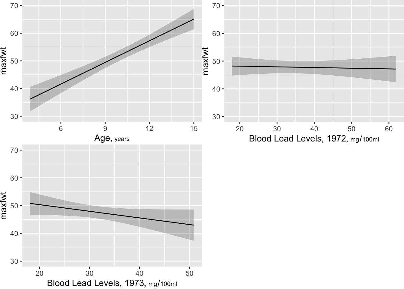

• To take control of which predictors are plotted, or to specify customized options: Q

ggplot(Predict(f, age))   # plot age effect, using default range,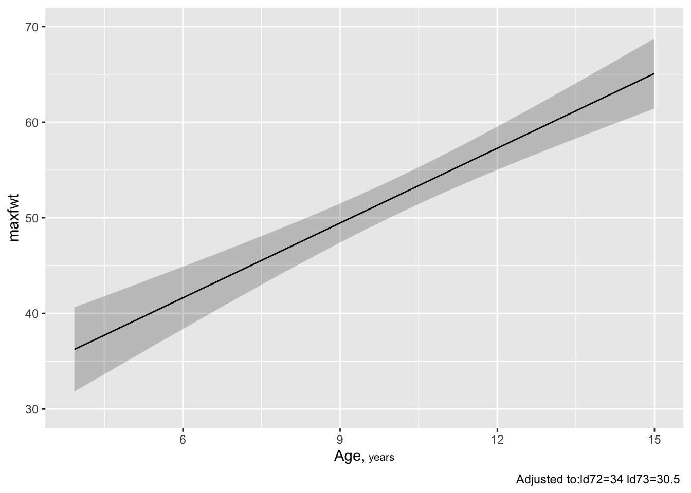

                          # 10th smallest to 10th largest age

R

ggplot(Predict(f, age=3:15))  # plot age=3,4,...,15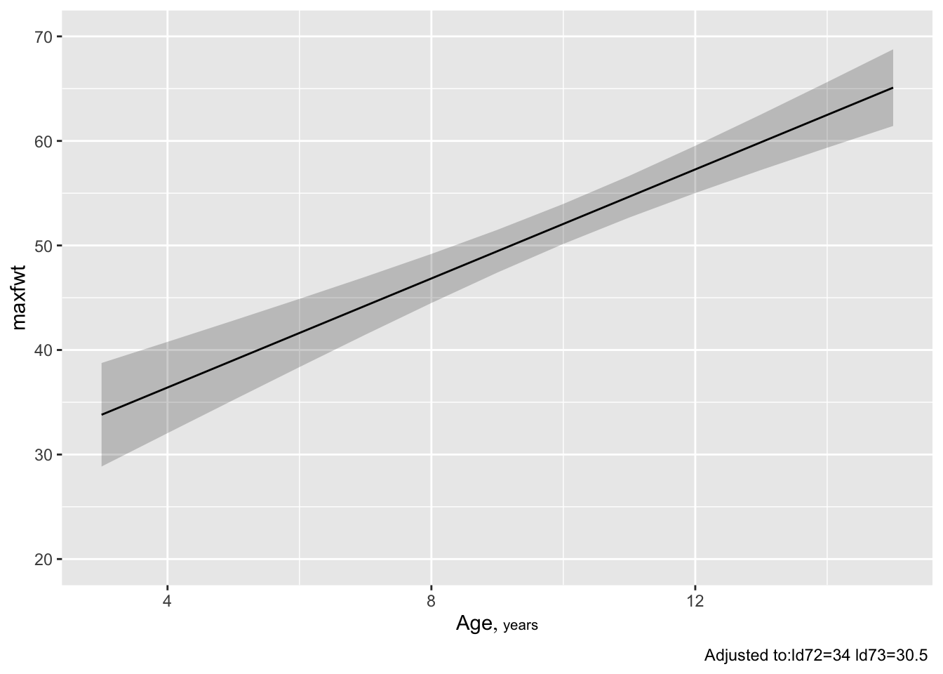 

S

ggplot(Predict(f, age=seq(3,16,length=150)))   # plot age=3-16, 150 points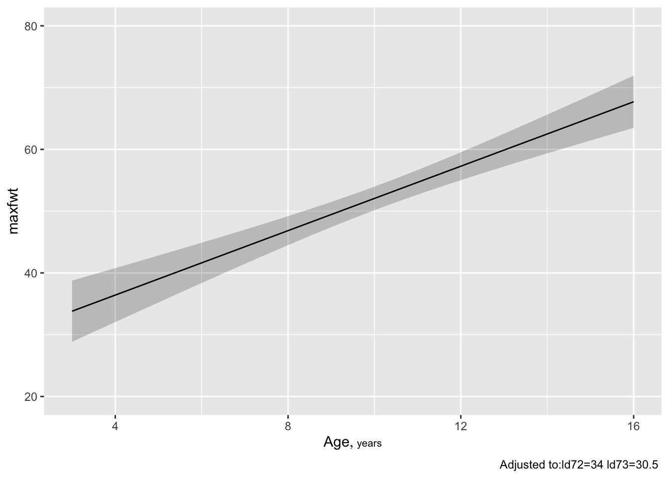 

• To get confidence limits for \(\hat{y}\): T

ggplot(Predict(f, age, conf.type='individual'))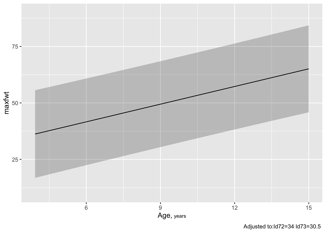

• To show both types of 0.99 confidence limits on one plot: U

p1 <- Predict(f, age, conf.int=0.99, conf.type='individual')
p2 <- Predict(f, age, conf.int=0.99, conf.type='mean')
p <- rbind(Individual=p1, Mean=p2)
ggplot(p)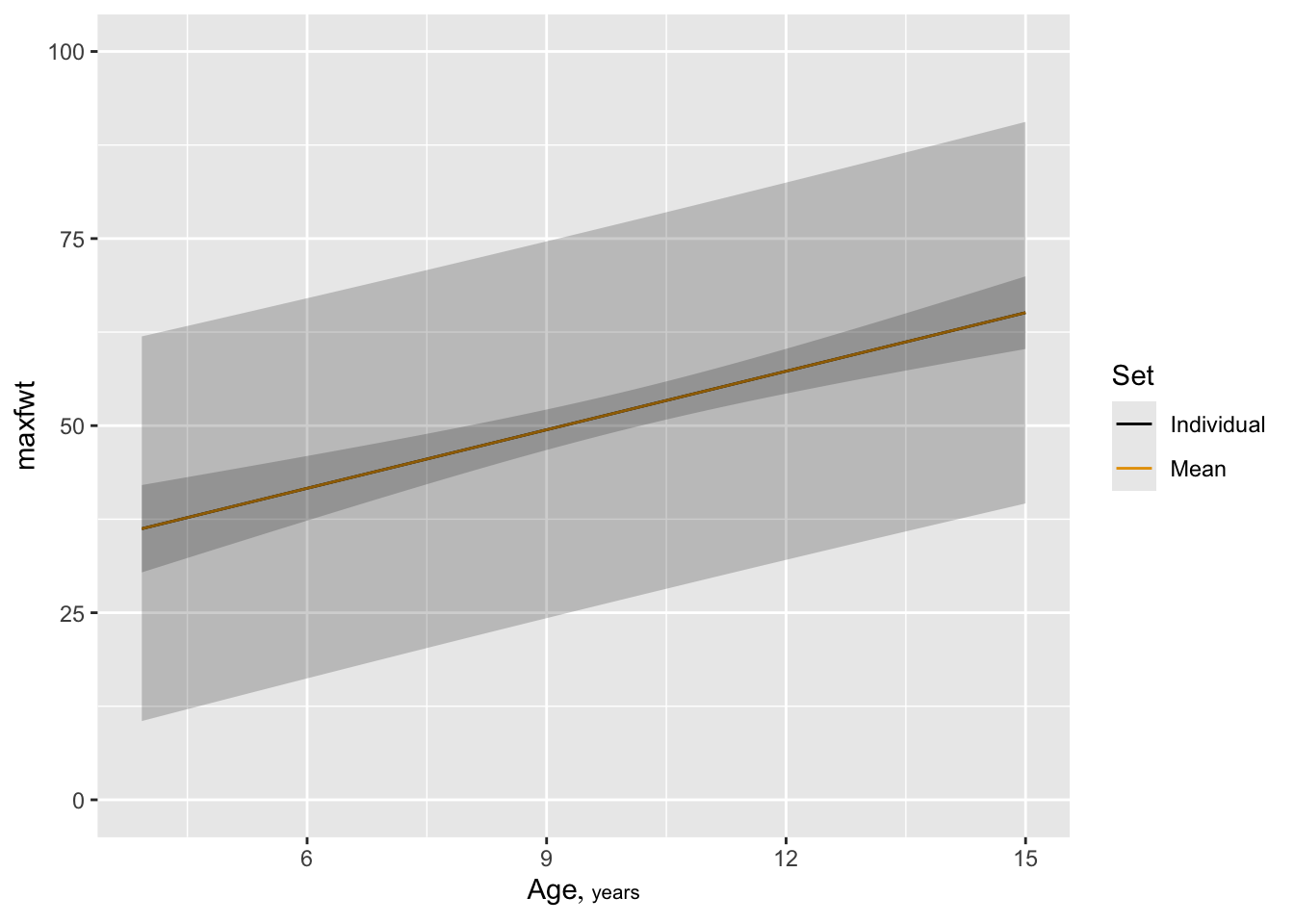

• Non-plotted variables are set to reference values (median and mode by default)
• To control the settings of non-plotted values use e.g. V

ggplot(Predict(f, ld73, age=3))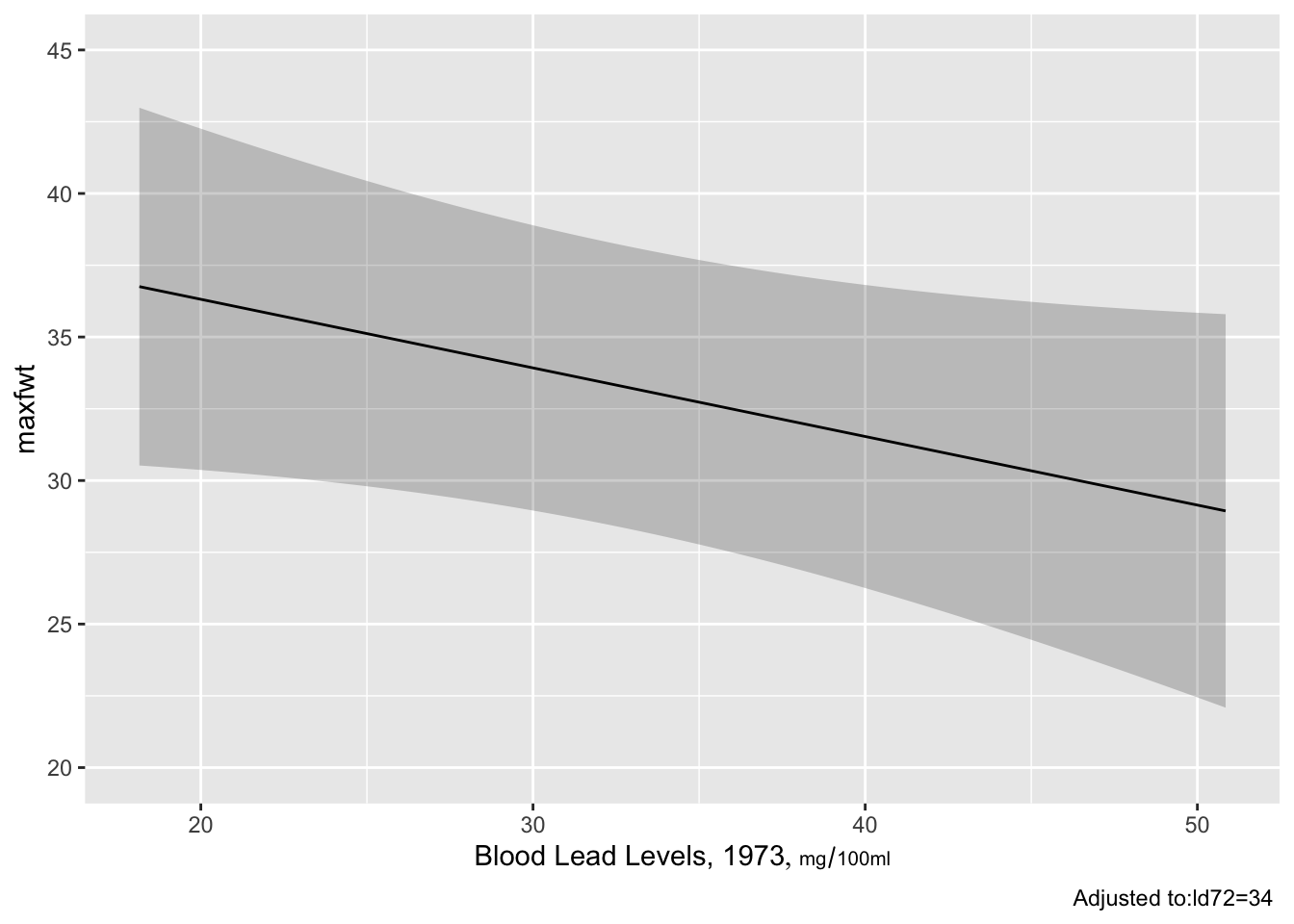

• To make separate lines for two ages: W

ggplot(Predict(f, ld73, age=c(3,9)))  # add ,conf.int=FALSE to suppress conf. bands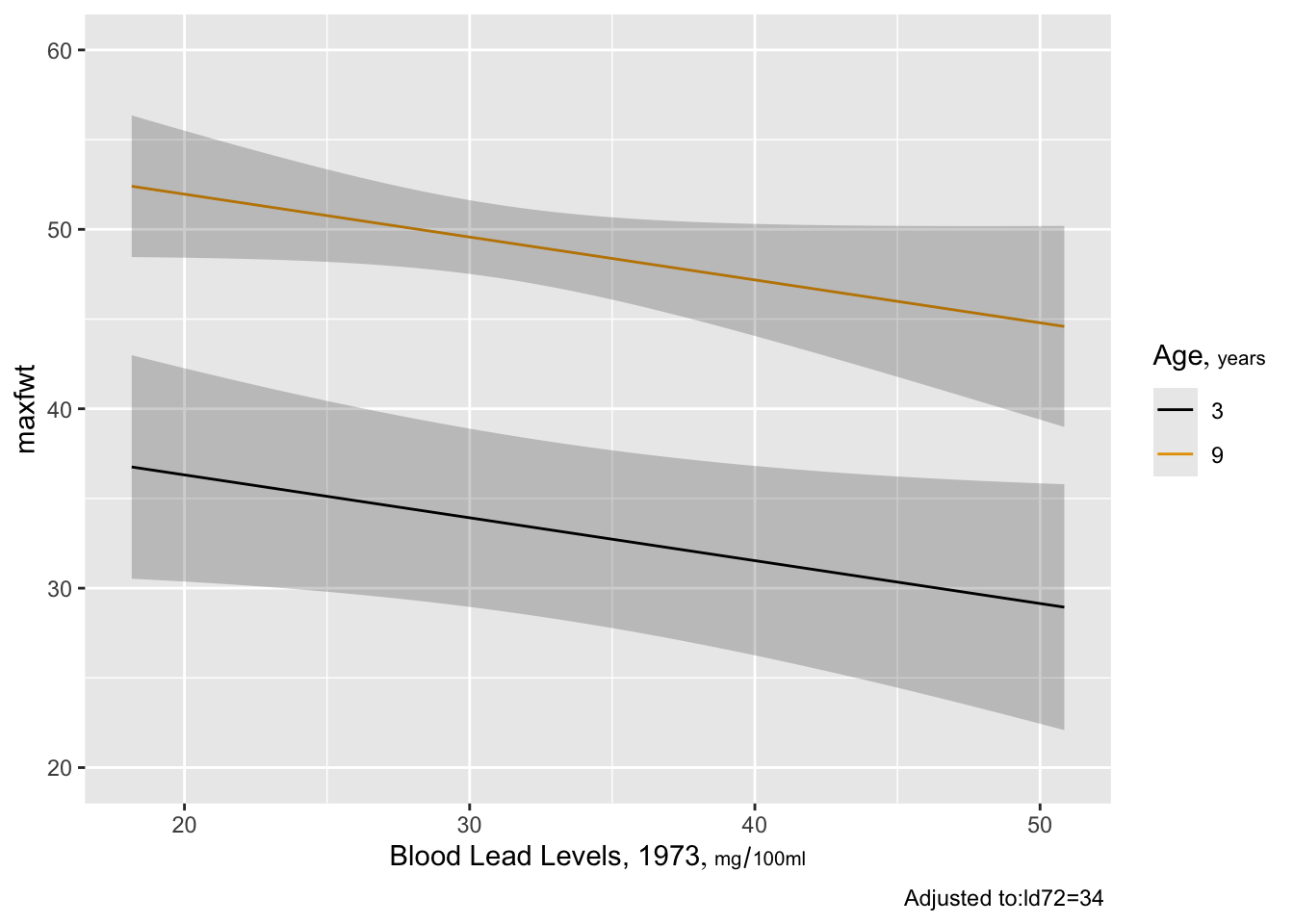

• To plot a 3-d surface for two continuous predictors against \(\hat{y}\); color coding for predicted mean maxfwt X

bplot(Predict(f, ld72, ld73))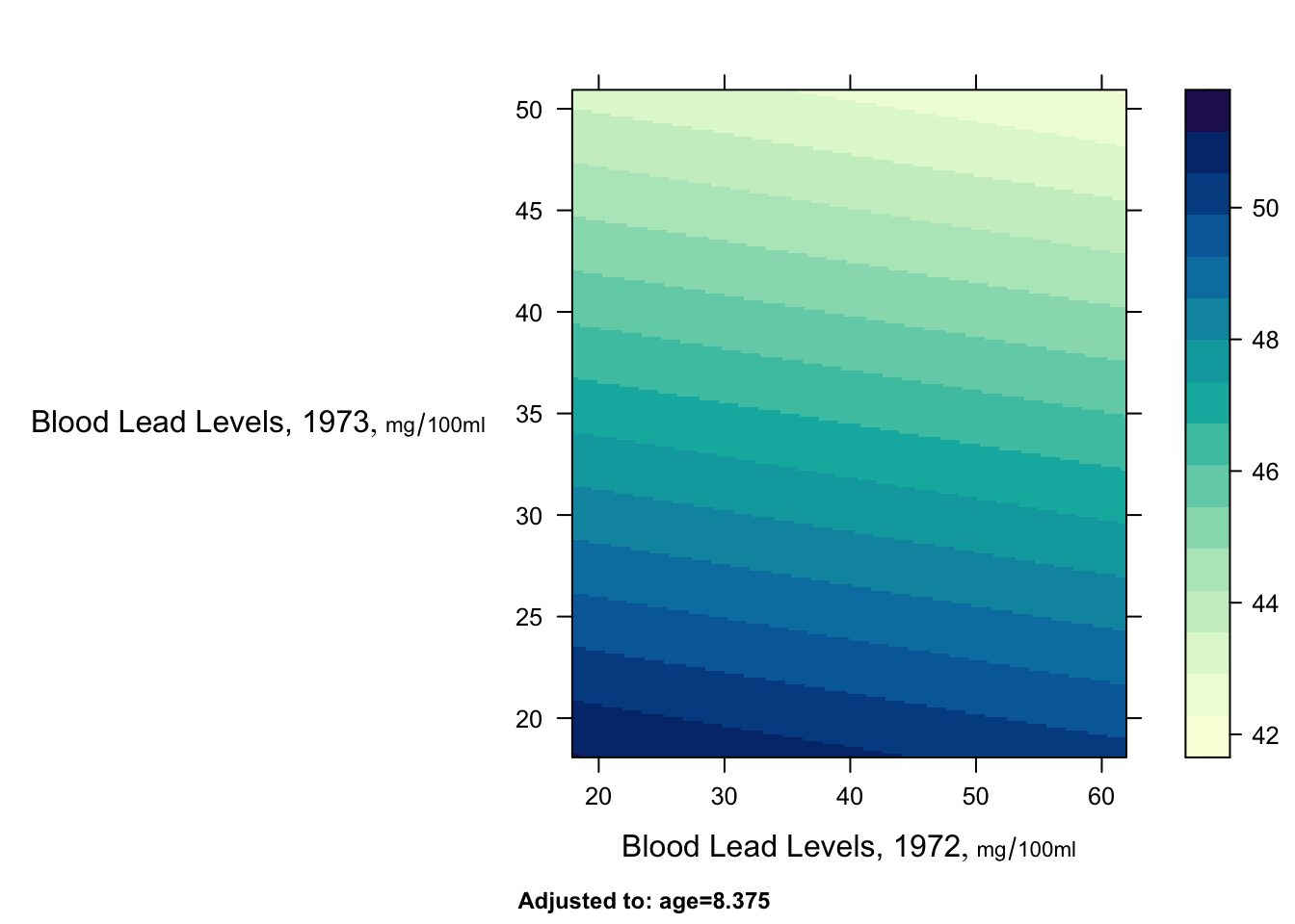

9.7 Nomograms: Overall Depiction of Fitted Models

Y

plot(nomogram(f))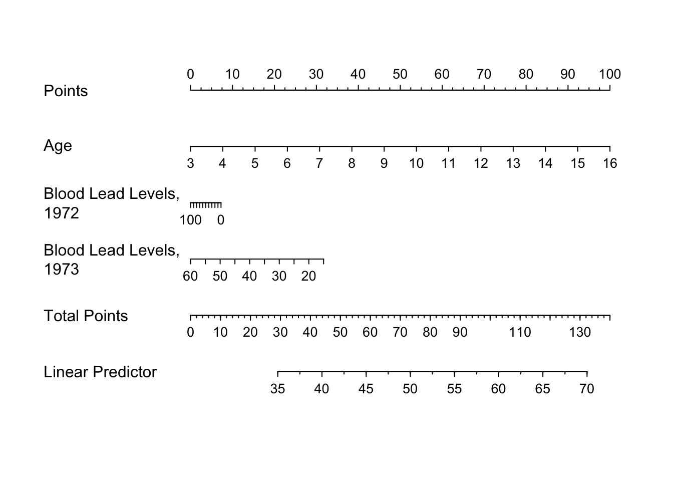

See this for excellent examples showing how to read such nomograms.

9.7.1 Point Estimates for Partial Effects

Z The summary function can compute point estimates and confidence intervals for effects of individual predictors, holding other predictors to selected constants. The constants you hold other predictors to will only matter when the other predictors interact with the predictor whose effects are being displayed.

How predictors are changed depend on the type of predictor:A

• Categorical predictors: differences against the reference (most frequent) cell by default

• Continuous predictors: inter-quartile-range effects by default The estimated effects depend on the type of model: B

• ols: differences in means

• logistic models: odds ratios and their logs

• Cox models: hazard ratios and their logs

• quantile regression: differences in quantiles

C

summary(f)         # inter-quartile-range effects 

Effects   Response: maxfwt
	Low	High	Δ	Effect	S.E.	Lower 0.95	Upper 0.95
age	6.167	12.02	5.854	15.2700	1.891	11.510	19.0200
ld72	27.000	43.00	16.000	-0.3936	1.251	-2.877	2.0900
ld73	24.000	37.00	13.000	-3.1070	1.722	-6.526	0.3123

summary(f, age=5)  # adjust age to 5 when examining ld72,ld73

Effects   Response: maxfwt
	Low	High	Δ	Effect	S.E.	Lower 0.95	Upper 0.95
age	6.167	12.02	5.854	15.2700	1.891	11.510	19.0200
ld72	27.000	43.00	16.000	-0.3936	1.251	-2.877	2.0900
ld73	24.000	37.00	13.000	-3.1070	1.722	-6.526	0.3123

                   # (no effect since no interactions in model)
summary(f, ld73=c(20, 40))  # effect of changing ld73 from 20 to 40

Effects   Response: maxfwt
	Low	High	Δ	Effect	S.E.	Lower 0.95	Upper 0.95
age	6.167	12.02	5.854	15.2700	1.891	11.510	19.0200
ld72	27.000	43.00	16.000	-0.3936	1.251	-2.877	2.0900
ld73	20.000	40.00	20.000	-4.7790	2.649	-10.040	0.4805

When a predictor has a linear effect, its slope is the one-unit change in \(Y\) when the predictor increases by one unit. So the following trick can be used to get a confidence interval for a slope: use summary to get the confidence interval for the one-unit change:

D

summary(f, age=5:6)    # starting age irrelevant since age is linear 

Effects   Response: maxfwt
	Low	High	Δ	Effect	S.E.	Lower 0.95	Upper 0.95
age	5	6	1	2.6080	0.3231	1.966	3.2490
ld72	27	43	16	-0.3936	1.2510	-2.877	2.0900
ld73	24	37	13	-3.1070	1.7220	-6.526	0.3123

There is a plot method for summary results. By default it shows 0.9, 0.95, and 0.99 confidence limits. E

spar(top=2)
plot(summary(f))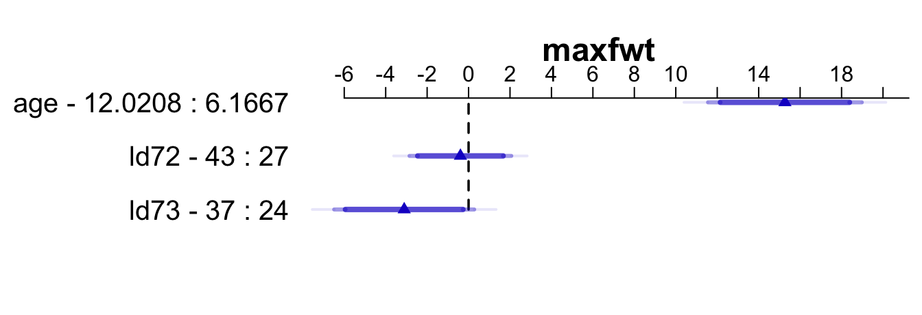

9.8 Getting Predicted Values

• Using predict F

predict(f, data.frame(age=3, ld72=21, ld73=21))

       1 
36.39448 

# must specify all variables in the model

predict(f, data.frame(age=c(3, 10), ld72=21, ld73=c(21, 47)))

       1        2 
36.39448 48.43618 

# predictions for (3,21,21) and (10,21,47)

newdat <- expand.grid(age=c(4, 8), ld72=c(21, 47), ld73=c(21, 47))
newdat

  age ld72 ld73
1   4   21   21
2   8   21   21
3   4   47   21
4   8   47   21
5   4   21   47
6   8   21   47
7   4   47   47
8   8   47   47

predict(f, newdat)     # 8 predictions

       1        2        3        4        5        6        7        8 
39.00232 49.43370 38.36278 48.79416 32.78911 43.22049 32.14957 42.58095 

G

predict(f, newdat, conf.int=0.95)  # also get CLs for mean 

$linear.predictors
       1        2        3        4        5        6        7        8 
39.00232 49.43370 38.36278 48.79416 32.78911 43.22049 32.14957 42.58095 

$lower
       1        2        3        4        5        6        7        8 
33.97441 46.23595 32.15468 43.94736 25.68920 36.94167 27.17060 38.86475 

$upper
       1        2        3        4        5        6        7        8 
44.03023 52.63145 44.57088 53.64095 39.88902 49.49932 37.12854 46.29716 

predict(f, newdat, conf.int=0.95, conf.type='individual')  # CLs for indiv.

$linear.predictors
       1        2        3        4        5        6        7        8 
39.00232 49.43370 38.36278 48.79416 32.78911 43.22049 32.14957 42.58095 

$lower
       1        2        3        4        5        6        7        8 
19.44127 30.26132 18.46566 29.27888 12.59596 23.30120 12.60105 23.31531 

$upper
       1        2        3        4        5        6        7        8 
58.56337 68.60609 58.25989 68.30944 52.98227 63.13979 51.69810 61.84659 

See also gendata.

• The brute-force way

# Model is b1 + b2*age + b3*ld72 + b4*ld73
b <- coef(f)
# For 3 year old with both lead exposures 21
b[1] + b[2]*3 + b[3]*21 + b[4]*21

Intercept 
 36.39448 

• Using Function function H

g <- Function(f)
g(age=c(3, 8), ld72=21, ld73=21)       # 2 predictions

[1] 36.39448 49.43370

g(age=3)              # 3 year old at median ld72, ld73

[1] 33.80449

9.9 ANOVA

• Use anova(fitobject) to get all total effects and individual partial effects
• Use anova(f,age,sex) to get combined partial effects of age and sex, for example
• Store result of anova in an object in you want to print it various ways, or to plot it:I

an <- anova(f)
an                     # same as print(an)

Analysis of Variance for maxfwt
	d.f.	Partial SS	MS	F	P
age	1	5907.535742	5907.535742	65.15	<0.0001
ld72	1	8.972994	8.972994	0.10	0.7538
ld73	1	295.044370	295.044370	3.25	0.0744
REGRESSION	3	7540.087710	2513.362570	27.72	<0.0001
ERROR	95	8613.750674	90.671060

anova(f, ld72, ld73)   # combine effects into a 2 d.f. test 

Analysis of Variance for maxfwt
	d.f.	Partial SS	MS	F	P
ld72	1	8.972994	8.972994	0.10	0.7538
ld73	1	295.044370	295.044370	3.25	0.0744
REGRESSION	2	747.283558	373.641779	4.12	0.0192
ERROR	95	8613.750674	90.671060

Enhanced output to better explain which parameters are being tested is available:

print(an, 'names')     # print names of variables being tested

Analysis of Variance for maxfwt
	d.f.	Partial SS	MS	F	P	Tested
age	1	5907.535742	5907.535742	65.15	<0.0001	age
ld72	1	8.972994	8.972994	0.10	0.7538	ld72
ld73	1	295.044370	295.044370	3.25	0.0744	ld73
REGRESSION	3	7540.087710	2513.362570	27.72	<0.0001	age,ld72,ld73
ERROR	95	8613.750674	90.671060

J

print(an, 'subscripts')# print subscripts in coef(f) (ignoring 

Analysis of Variance for maxfwt
	d.f.	Partial SS	MS	F	P	Tested
age	1	5907.535742	5907.535742	65.15	<0.0001	1
ld72	1	8.972994	8.972994	0.10	0.7538	2
ld73	1	295.044370	295.044370	3.25	0.0744	3
REGRESSION	3	7540.087710	2513.362570	27.72	<0.0001	1-3
ERROR	95	8613.750674	90.671060

                       # the intercept) being tested
print(an, 'dots')      # a dot in each position being tested

Analysis of Variance for maxfwt
	d.f.	Partial SS	MS	F	P	Tested
age	1	5907.535742	5907.535742	65.15	<0.0001	•
ld72	1	8.972994	8.972994	0.10	0.7538	•
ld73	1	295.044370	295.044370	3.25	0.0744	•
REGRESSION	3	7540.087710	2513.362570	27.72	<0.0001	•••
ERROR	95	8613.750674	90.671060

9.10 Study Questions

Section 9.6

1. What about our ANOVA is consistent with the color image plot for the two continuous lead exposure predictors?

Section 9.7

1. Define the IQR effect of ld73.

Harrell, F. E. (2020). rms: R functions for biostatistical/epidemiologic modeling, testing, estimation, validation, graphics, prediction, and typesetting by storing enhanced model design attributes in the fit. https://hbiostat.org/R/rms