Regression Modeling Strategies

Author

Affiliation

Department of Biostatistics
School of Medicine
Vanderbilt University

Published

May 16, 2026

flowchart LR
rms[Multivariable Model Development] --> est[Estimation] --> pred[Prediction] --> val[Validation]

Preface

A statistical model is a set of assumptions or constraints on possible features of the data generating process that permit us to compute estimates that we believe will properly represent or predict phenomena of interest. A regression model is a statistical model with indentifiable unknown parameters and specific constraints such as additivity allowing one to isolate the effects or predictive contributions of individual features. All regression models have assumptions or constraints that must approximately hold for (1) findings from model-based analyses not to have alternate explanations, (2) statistical power to detect associations be optimized, (3) estimates about unknowns to have optimum precision, and (4) predictions to be accurate.

There are four principal types of assumptions of regression models:

linearity of effects of predictors
additivity of effects of multiple predictors
absolute distributional assumptions
relative distributional assumptions

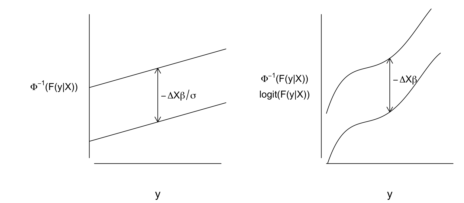
Absolute distributional assumptions are made for parametric regression models. These assume a specific distribution for the dependent variable $Y$ given specific predictor $X$ values. Relative distributional assumptions pertain to how the shape of the $Y$ distribution for one set of $X$ values relates to the shape for other values of $X$ (sometimes called a proportionality assumption). Semiparametric regression models only make the second kind of distributional assumption.

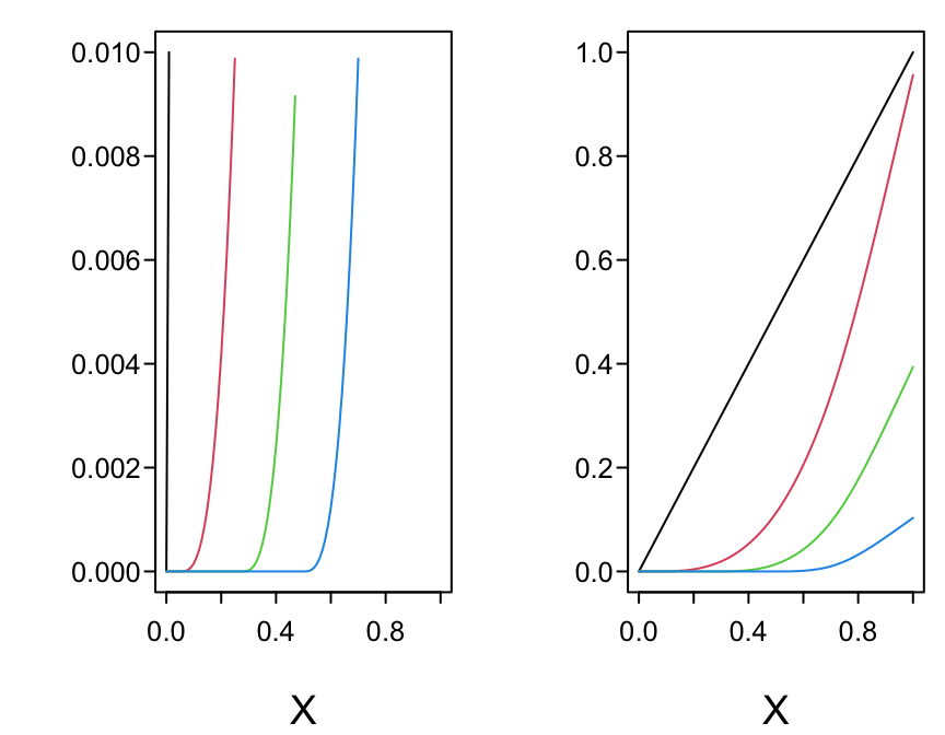
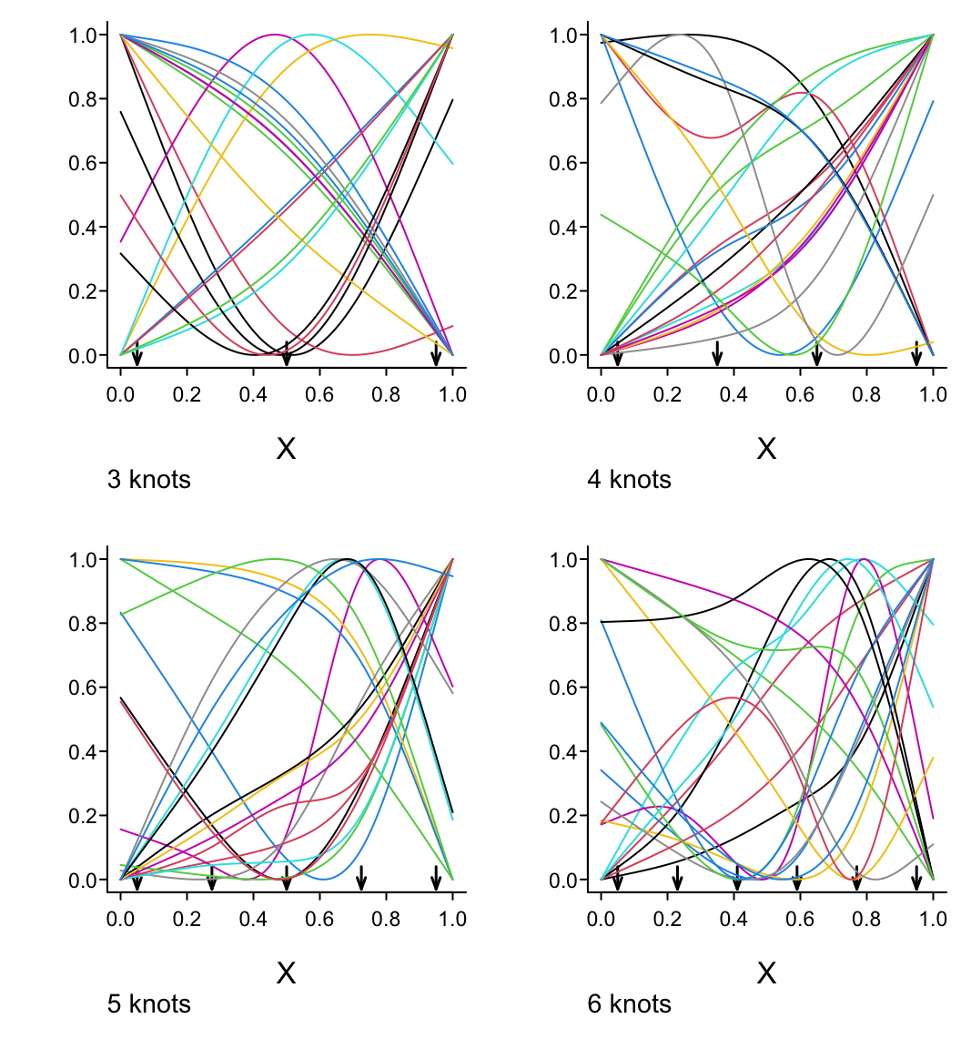
This course emphasizes methods for assessing and satisfying assumption types 1, 2, and 4. Less attention is paid to assumption 3 due to the course’s emphasis on semiparametric models. Practical but powerful tools are presented for validating model assumptions, relaxing assumptions, and presenting model results. This course provides methods for estimating the shape of the relationship between predictors and response using the widely applicable method of augmenting the design matrix using restricted cubic splines. Even when assumptions are satisfied, overfitting can ruin a model’s predictive ability for future observations. Methods for data reduction will be introduced to deal with the common case where the number of potential predictors is large in comparison with the number of observations. Methods of model validation (bootstrap and cross-validation) will be covered, as well as quantifying predictive accuracy and predictor importance, modeling interaction surfaces, efficiently recovering partial covariable data by using multiple imputation, variable selection, overly influential observations, collinearity, and shrinkage, and a brief introduction to the R rms package for handling these problems. The methods covered will apply to almost any regression model, including ordinary least squares, longitudinal models, logistic regression models, ordinal regression, quantile regression, longitudinal data analysis, and survival models. Statistical models will be contrasted with machine learning so that the student can make an informed choice of predictive tools.

Target Audience

Those who may benefit include statisticians and persons from other quantitative disciplines who are interested in multivariable regression analysis of univariate and longitudinal responses; in developing, validating, and graphically describing multivariable predictive models; and in covariable adjustment in clinical trials and observational data analyses. The course will be of particular interest to applied statisticians and developers of applied statistics methodology, graduate students, clinical and pre-clinical biostatisticians, health services and outcomes researchers, econometricians, psychometricians, and quantitative epidemiologists. A good command of ordinary multiple regression is a prerequisite.

Learning Goals

Students will

be able to fit multivariable regression models:
- accurately
- in a way the sample size will allow, without overfitting
- uncovering complex non–linear or non–additive relationships
- testing for and quantifying the association between one or more predictors and the response, with possible adjustment for other factors
- making maximum use of partial data rather than deleting observations containing missing variables
be able to validate models for predictive accuracy and to detect overfitting and understand problems caused by overfitting.
learn techniques of “safe data mining” in which significance levels, confidence limits, and measures such as $R^2$ have the claimed properties.
learn how to interpret fitted models using both parameter estimates and graphics
learn about the advantages of semiparametric ordinal models for continuous $Y$
learn about some of the differences between frequentist and Bayesian approaches to statistical modeling
learn differences between machine learning and statistical models, and how to determine the better approach depending on the nature of the problem

Course Philosophy

Modeling is the endeavor to transform data into information and information into either prediction or evidence about the data generating mechanism¹
Models are usually the best multivariable descriptive statistics
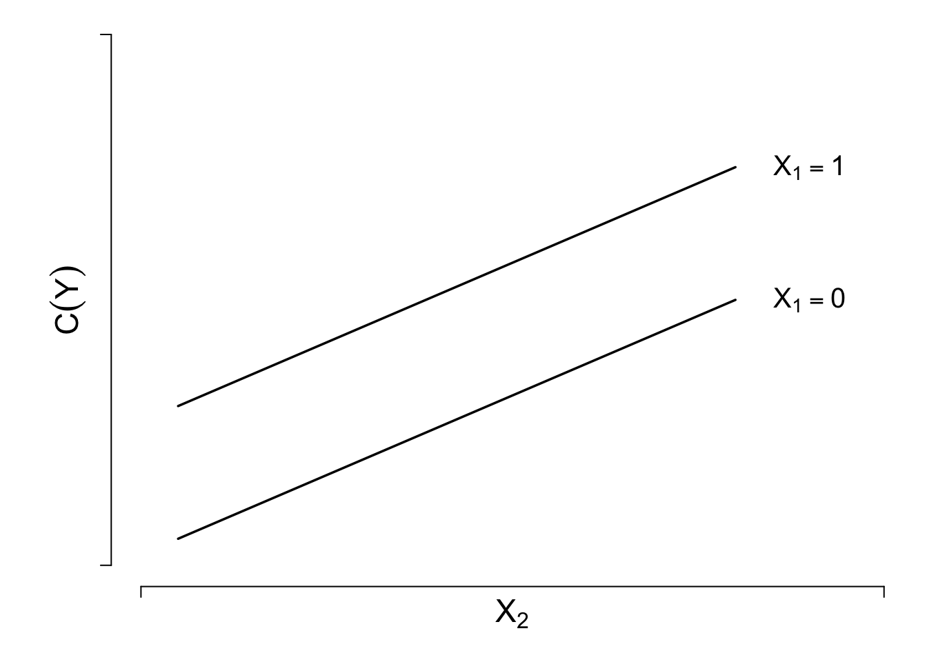
- adjust for one variable while displaying the association with $Y$ and another variable
- multivariable descriptive statistics usually do not work when relating > 2 variables
Satisfaction of model assumptions improves precision and increases statistical power
- Be aware of assumptions, especially those mattering the most
It is more productive to make a model fit step by step (e.g., transformation estimation) than to postulate a simple model and find out what went wrong
- Model diagnostics are often not actionable
- Changing the model in reaction to observed patterns $\uparrow$ uncertainty but is reflected by an apparent $\downarrow$ in uncertainty
Graphical methods should be married to formal inference
Overfitting occurs frequently, so data reduction and model validation are important
Software without multiple facilities for assessing and fixing model fit may only seem to be user-friendly
Carefully fitting an improper model is better than badly fitting (and overfitting) a well-chosen one
- E.g. small $N$ and overfitting vs. carefully formulated right hand side of model
Methods which work for all types of regression models are the most valuable.
In most research projects the cost of data collection far outweighs the cost of data analysis, so it is important to use the most efficient and accurate modeling techniques, to avoid categorizing continuous variables, and to not remove data from the estimation sample just to be able to validate the model.
- A $100 analysis can make a $1,000,000 study worthless.
The bootstrap is a breakthrough for statistical modeling and model validation.
Bayesian modeling is ready for prime time.
- Can incorporate non-data knowledge
- Provides full exact inferential tools even when penalizing $\beta$
- Rational way to account for model uncertainty
- Direct inference: evidence for all possible values of $\beta$
- More accurate way of dealing with missing data
Using the data to guide the data analysis is almost as dangerous as not doing so.
A good overall strategy is to decide how many degrees of freedom (i.e., number of regression parameters) can be "spent", where they should be spent, to spend them with no regrets. See the excellent text Clinical Prediction Models (Steyerberg, 2019)

¹ Thanks to Drew Levy for ideas that greatly improved this section.

Key Messages of the Course

A fundamental RMS principle is to aim for “methods that enable an analyst to develop models that will make accurate predictions of responses for future observations.” The RMS program (philosophy, methodology, tools) is dedicated to this, as well as to estimating shapes of predictor effects while adjusting for other predictors.
Phantom degrees of freedom : Information about the relationship between the dependent variable and candidate predictors introduced into model specification or model selection that is not later properly accounted for in the variance estimates and inference that goes into the ultimate report of analysis results. Put another way: assessments made in model development and then later elided that compromise the fidelity of standard errors, alpha, Type-I assertion probability $\alpha$, etc. It is ‘phantom’ not only because it disappears, but also because this information continues to haunt the analysis, typically with overconfidence.
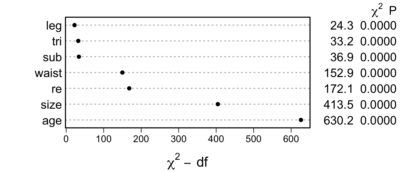
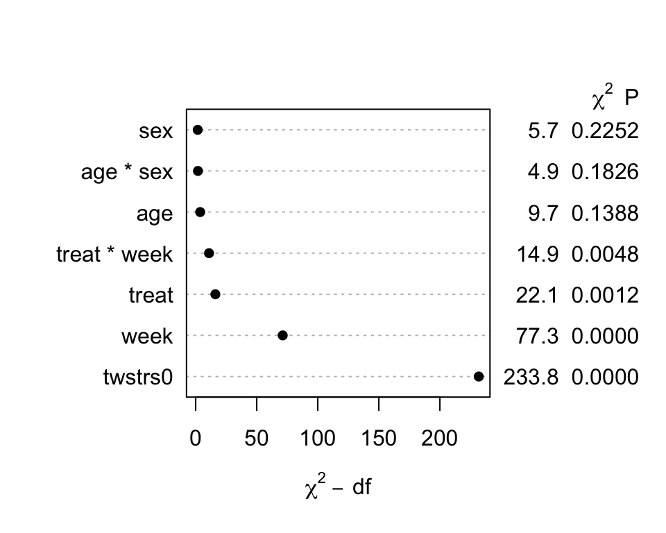
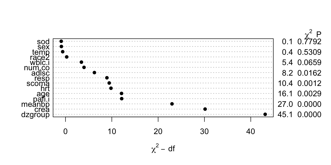
$\chi^{2}$ - df : The magnitude of predictive signal (which is proportional to $n$), chance-corrected by subtracting the expected amount of apparent explanatory information that occurs when there is no association (which is the degrees of freedom, i.e., effective number of parameters and is constant, i.e., does not depend on $n$).
Chunk tests : Simultaneous or aggregate assessment of the importance (e.g., proportion of total variance explained) of collinear or dependent (e.g. related polynomial or interaction) terms or a group of non-collinear candidate predictors. Important for making coherent judgments.
Spending df’s : Given a fixed amount of information in the data available for the analysis there is an ‘information budget’ that should be used judiciously: more important predictors should represented in a richer way (e.g. make the number of knots in splines proportional to the overall importance and complexity in the variable) than predictors that are less important. “Spending df’s with no regrets”: to preserve the operating characteristics of formal inference, once assessed in the modeling process even the less important candidate predictors should remain in view and not elided. All candidate predictors get a portion of the ‘df budget’, but to a varying extent based on their predictive potential.
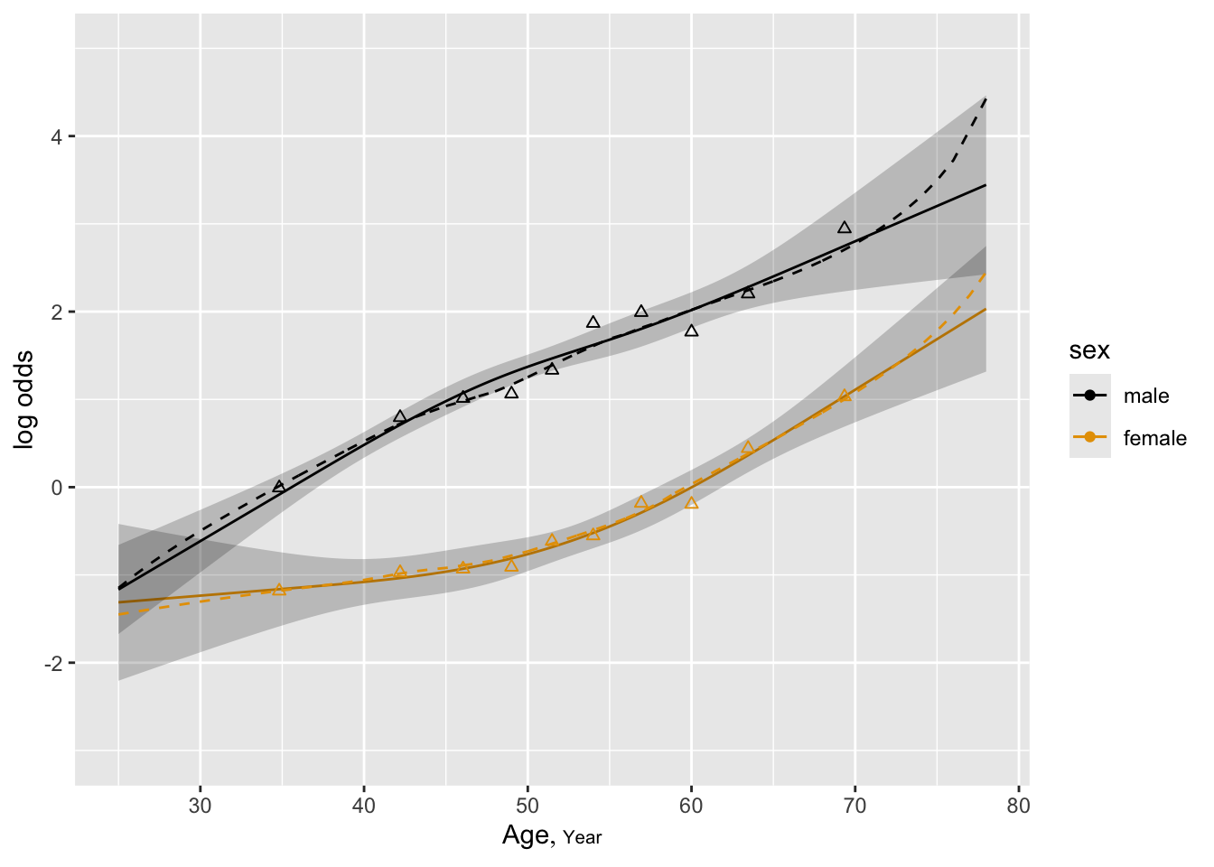
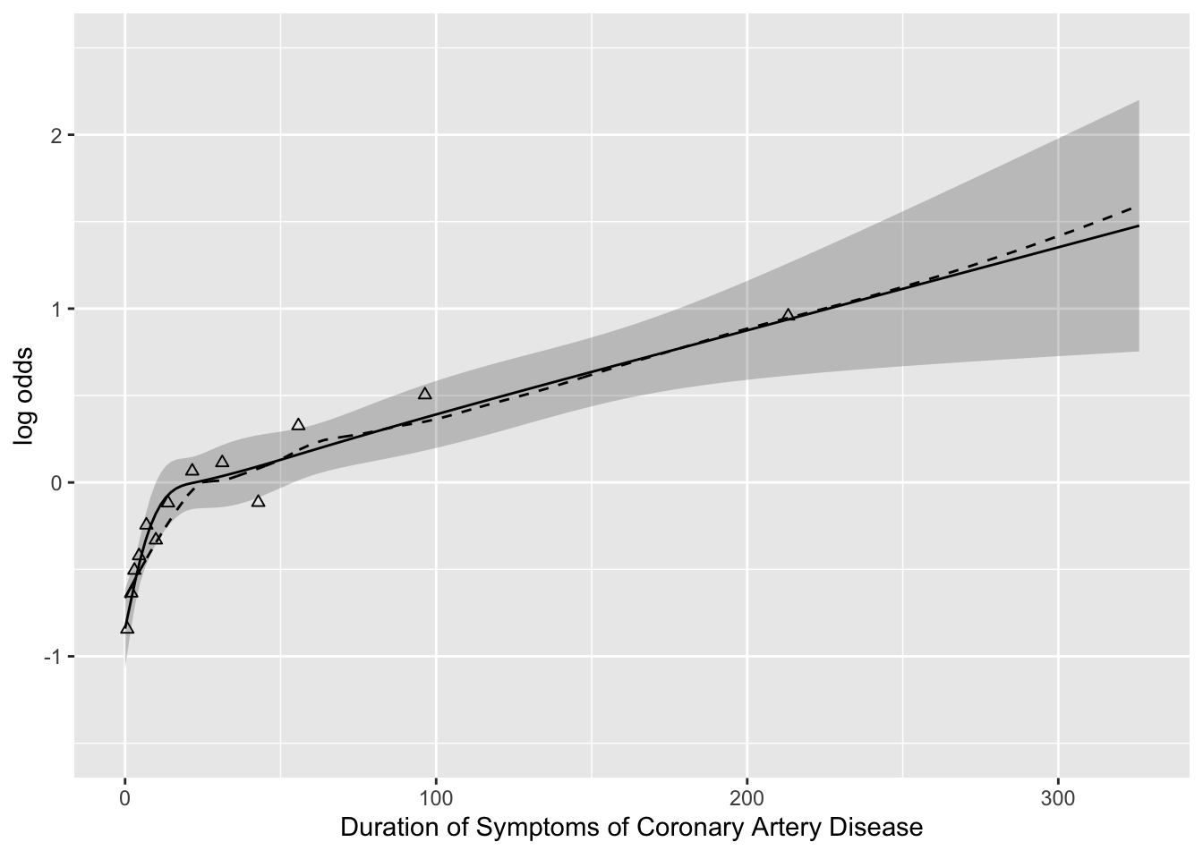
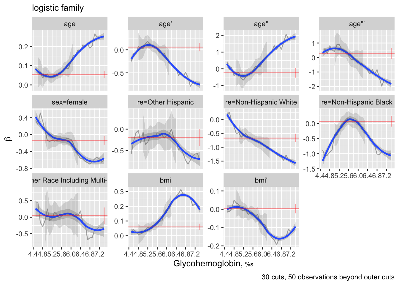
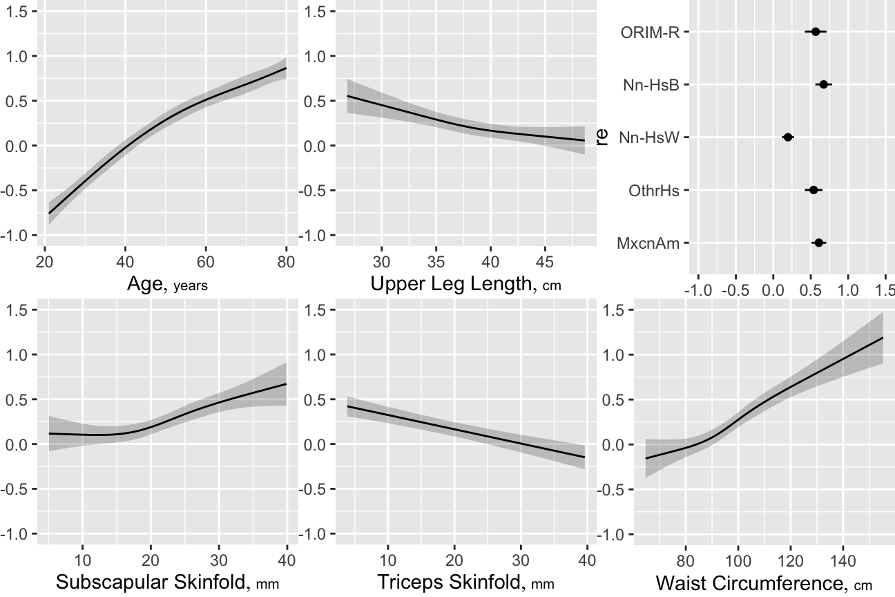
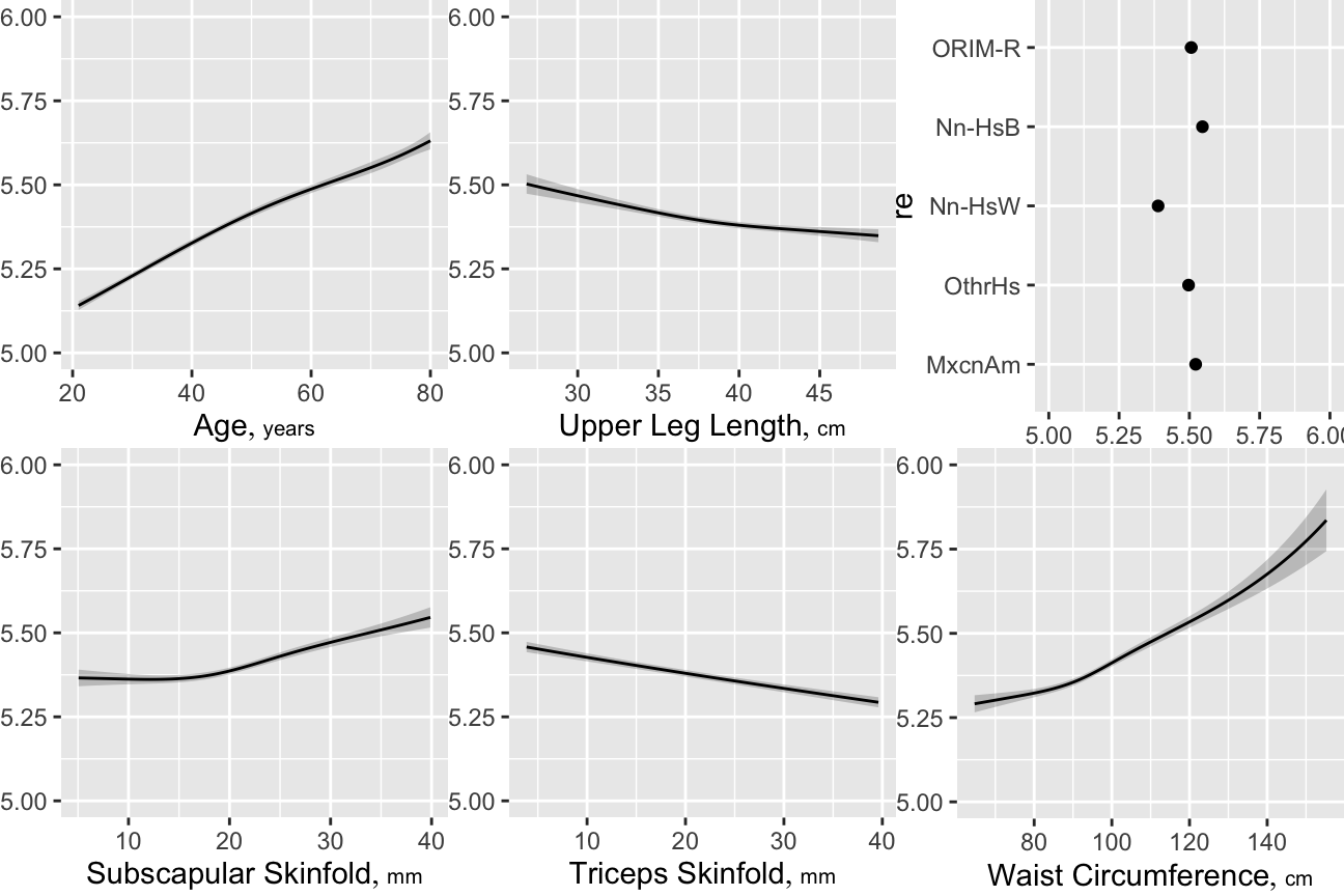
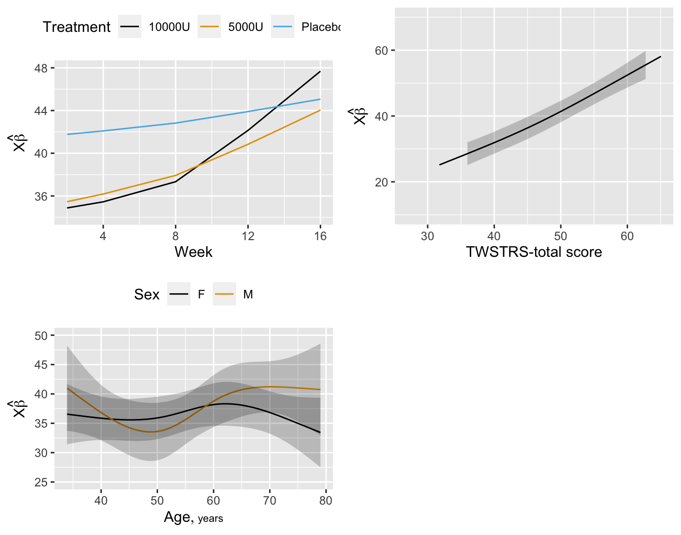
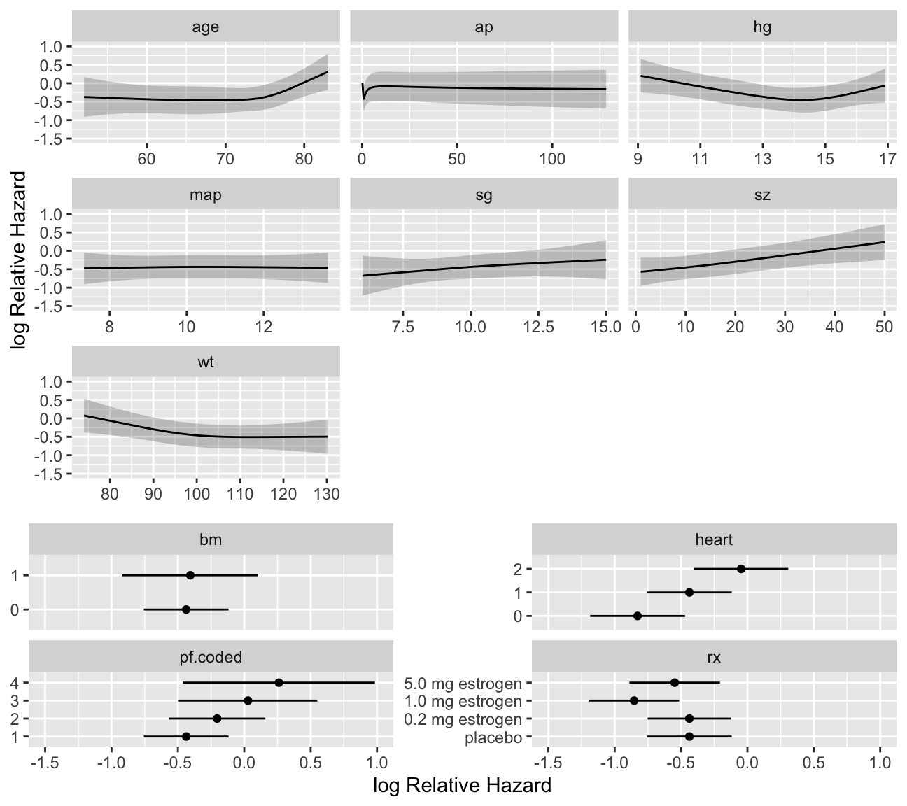
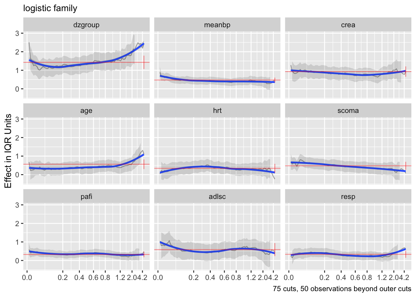
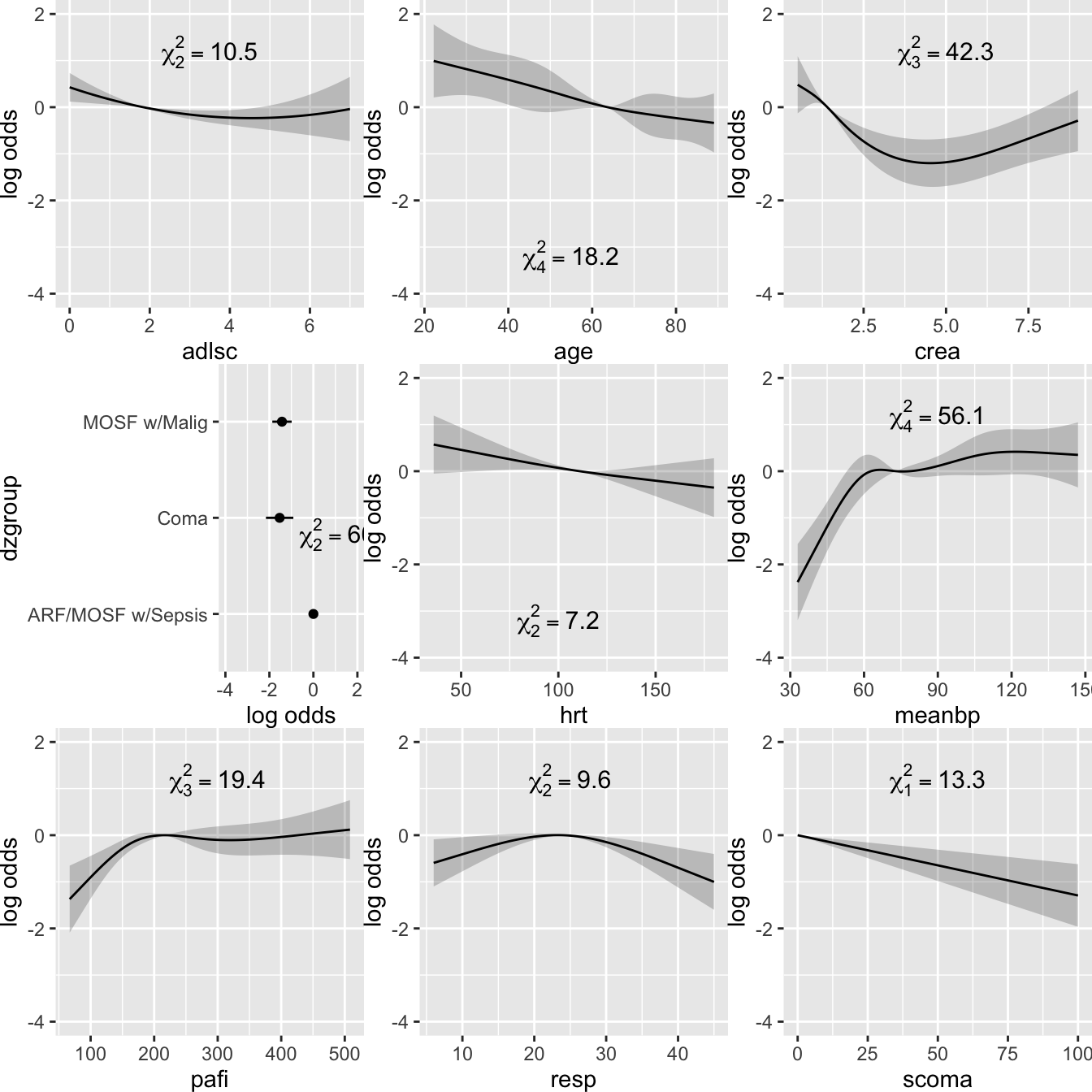
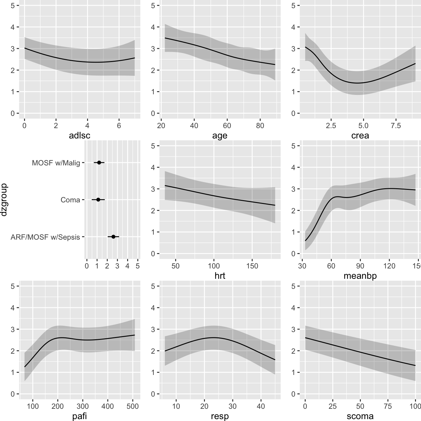
Partial plots: Pay special attention to partial plots. Partial plots reveal important information about where the information is in predicting the dependent variable. Partial plots elucidate the form and strength of individual predictors (independent of covariate effects) and can reveal the structure in the data and where the information is situated in the model.
Be aware that cognitive biases — and an analysts’ interests, incentives and ethics — are all also a latent (often insidious) part of the overall analysis and reporting process. Be honest with others and yourself.
Consider RMS as practicing a craft, and the RMS text book as the foundational treatise for the craft. Get, read–and periodically re-read–the textbook. There is a lot in the book not covered in the short course. Reading the text will help by providing students a comprehensive tool set, and reinforce the overall coherence in RMS. And there is also a lot of wisdom throughout the textbook.

Written by Drew Levy

Annotating the Notes

For information about adding annotations, comments, and questions inside the text click here: Comments

Symbols Used in the Right Margin of the Text

in the right margin is a hyperlink to a YouTube video related to the subject.
is a hyperlink to the discussion topic in datamethods.org devoted to the specific topic. You can go directly to the discussion about chapter n by going to datamethods.org/rmsn.
An audio player symbol indicates that narration elaborating on the notes is available for the section. Red letters and numbers in the right margin are cues referred to within the audio recordings.
blog in the right margin is a link to a blog entry that further discusses the topic.

Other Information

4-day course notes: hbiostat.org/course/rms
4-day course syllabus and daily schedules: hbiostat.org/doc/rms/desc.html
Master RMS notes: hbiostat.org/rmsc
Instats participants: use the Forum for the course on Instats.org
Datamethods Long-term Discussion board and hints for registering
How to annotate and pose questions on web pages
- Do this only on the master RMS notes
X and BlueSky: #rmscourse
Publicly available videos of the short course
- Four hour short course from useR!2022
BBR course
Go directly to a YouTube video for RMS Session n by going to bit.ly/yt-rmsn
Study questions at the end of selected chapters
Statistical papers written for clinical researchers
RMS overview and template for statistical analysis plan
Statistical Thinking blog: fharrell.com
Glossary of statistical terms: hbiostat.org/glossary
R Workflow: hbiostat.org/rflow

Acknowledgements

A number of individuals who are key to my career and to the development of RMS were acknowledged in the preface to the $2^\text{nd}$ edition of Regression Modeling Strategies. In particular, David Hurst, the first Chair of the Department of Biostatistics at the University of Alabama in Birmingham, was singularly responsible for my entering the field of biostatistics. I also wish to thank Drew Levy and Madeline Bauer for critical reading of these course notes and providing a large number of constructive comments that made the notes significantly better.

R Packages

To be able to run all the examples in the book, install current versions of the following CRAN packages:

Hmisc, rms, data.table, nlme, rmsb, ggplot2
kableExtra, pcaPP, VGAM, MASS, leaps, rpart

License

Regression Modeling Strategies Course is licensed under a Creative Commons Attribution-NonCommercial-ShareAlike 4.0 International License.
Based on a work at https://hbiostat.org/rmsc.

Update History

Date	Sections	Changes
2026-05-16	Model Robustness	New subsection of robustness of model
2026-05-07	Hypothesis Testing, Estimation, and Prediction	New subsection on estimation qualities
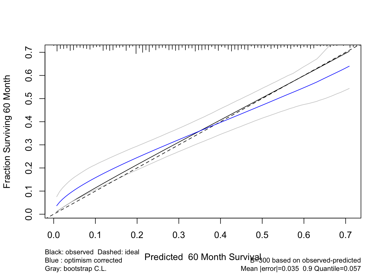
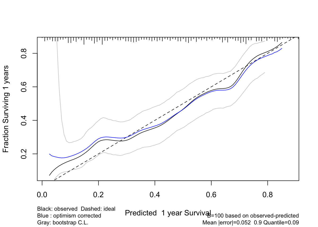
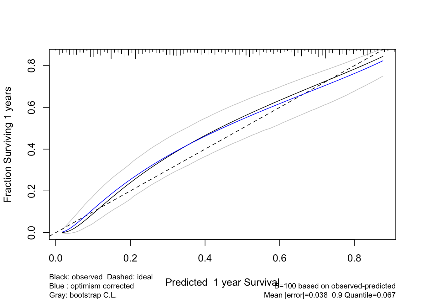
2025-05-26	Confidence Intervals for Overfitting-Corrected Model Performance Measures	New subsubsection on confidence intervals for bootstrap bias-corrected accuracy measures, added limits in various validation and calibration examples
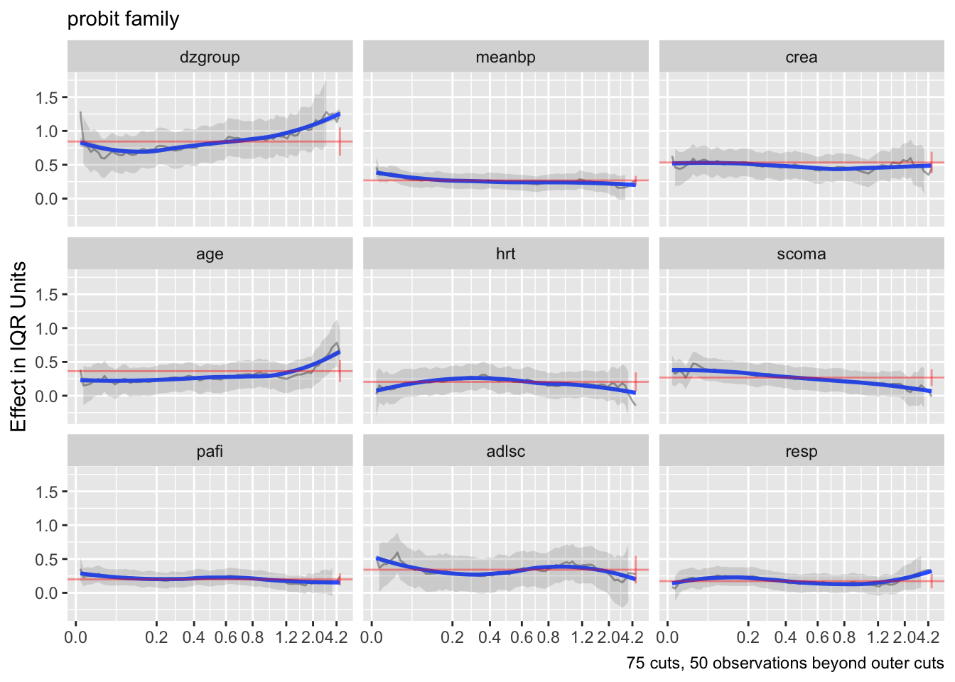
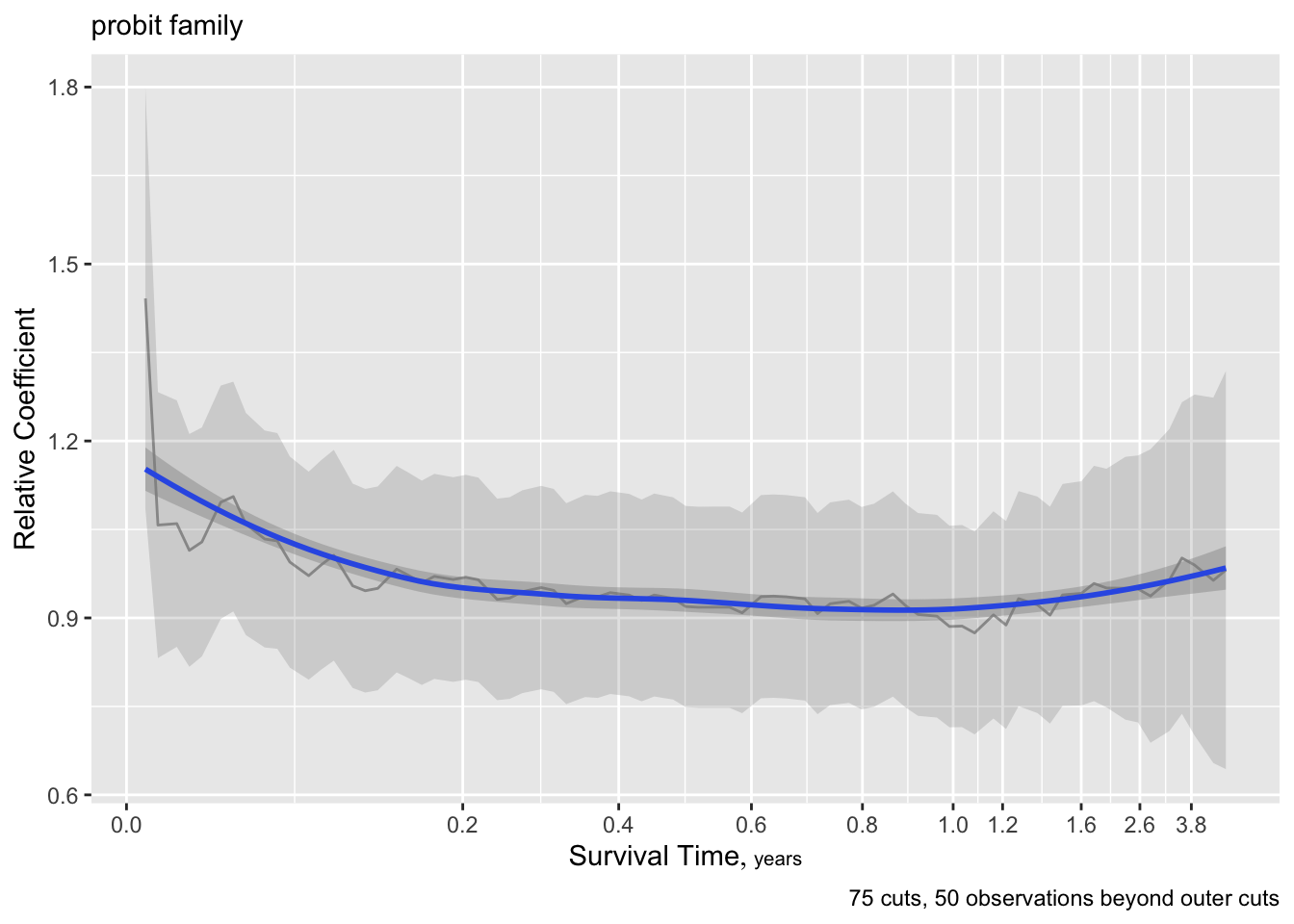
2025-03-10	Checking Assumptions of OLS and Other Models	Added usage of `ordParallel` and `Olinks`
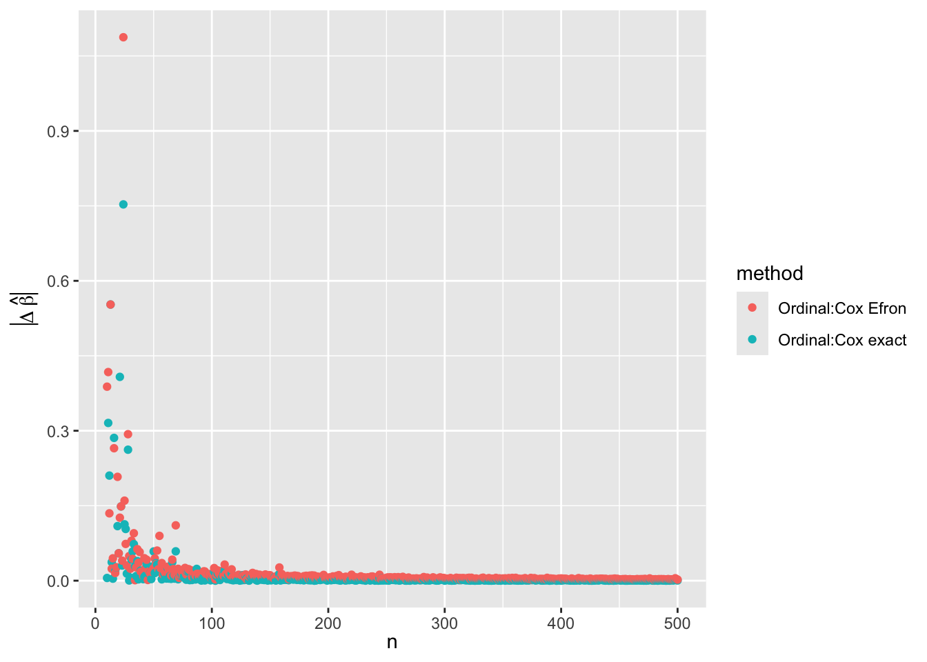
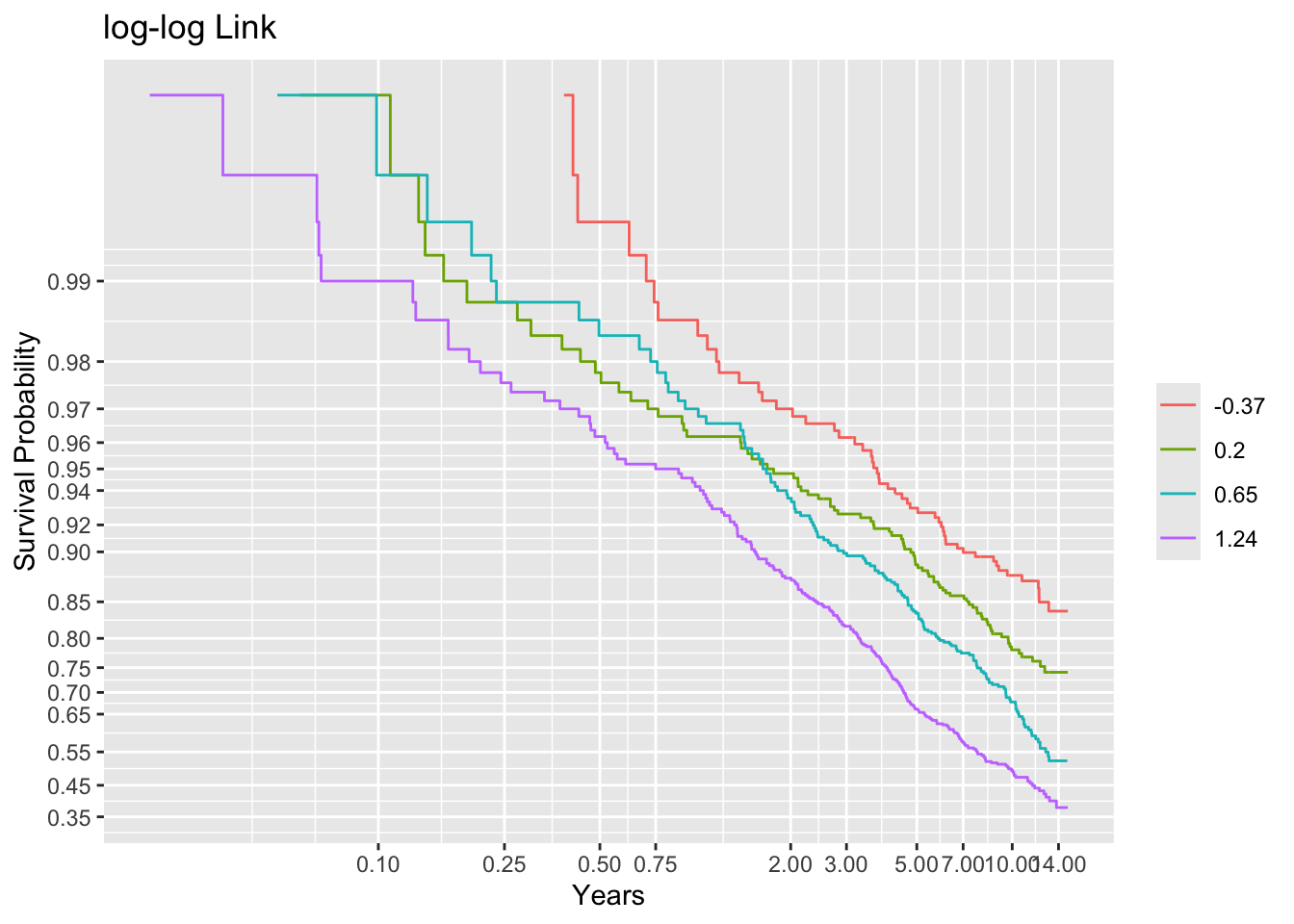
2025-03-01	25 Ordinal Semiparametric Regression for Survival Analysis	New chapter on survival analysis with ordinal regression
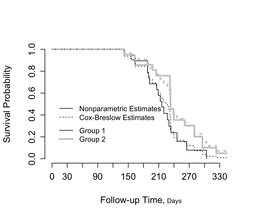
2025-02-23	Assessment of Model Fit	Replaced some `survplot()`s with the new `ggplot.npsurv` method
2025-01-03	Contrasts and Model Reparameterization	New section on reparameterizing models to make contrast coefficients and set up for profile likelihood
2024-11-18	Pre-Processing of the Design Matrix	New section on preprocessing using QR and how to adjust the Hessian
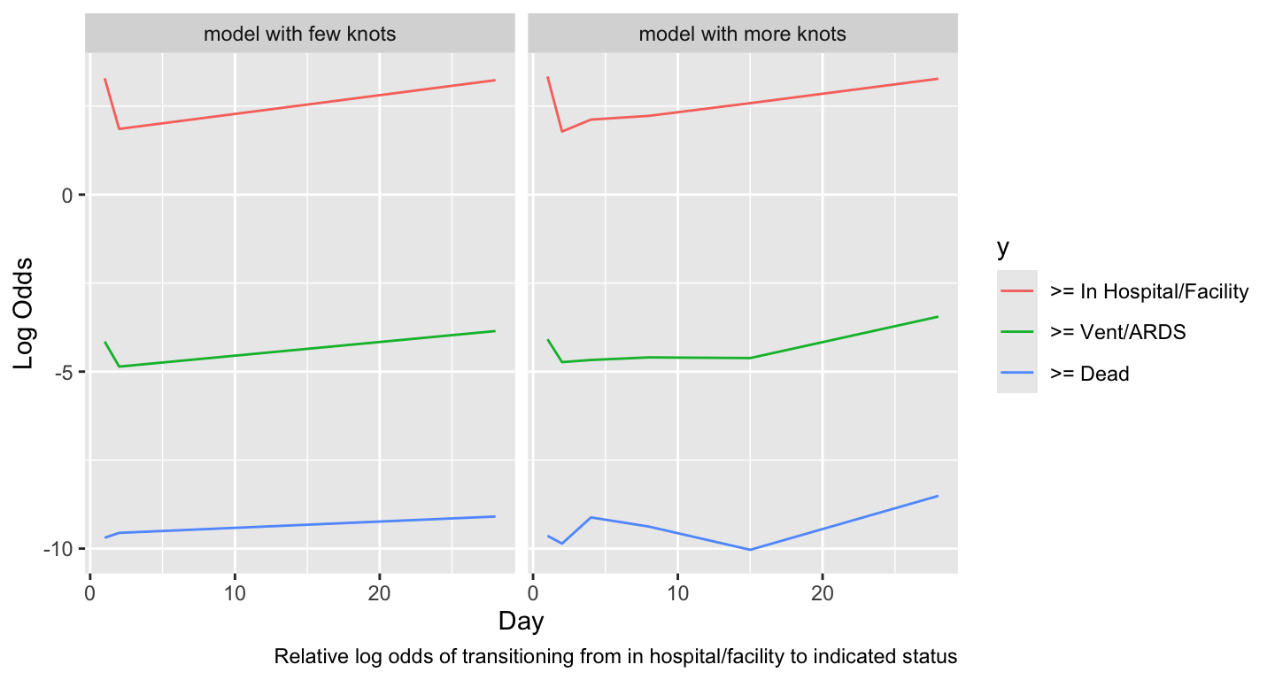
2024-11-14	Relaxing Linearity Assumption for Continuous Predictors	Added link to new interactive demo
2024-10-13	Bayesian Modeling	Expanded to include collapsible section on uncertainty in model performance metrix, plus problems with CLT and $\delta$-method
2024-08-11	Preface	Added Drew Levy’s key messages
2024-08-02	Validation of Bayesian Models	New subsection on validation issues in Bayesian modeling
2024-04-21	Bayesian Logistic Model Example	Updated `blrm` from using `keepsep` to `pcontrast`
2024-03-03	Validation of Data Reduction	New section of validatiion of data reduction
2024-02-18	Contrasts	New section on contrasts
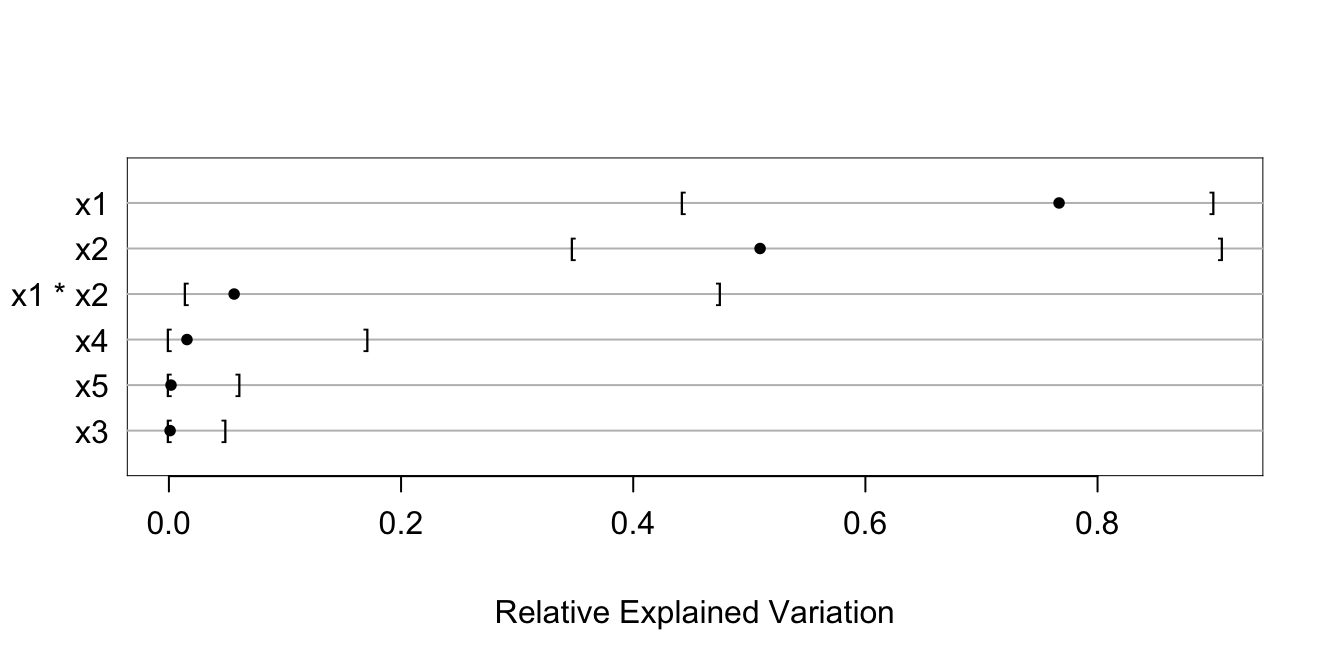
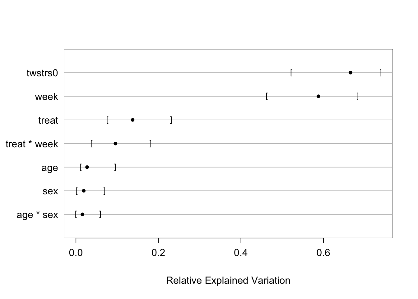
2023-09-17	Relative Explained Variation	New subsection on relative explained variation
2023-08-02	Predictive Mean Matching With Constraints	New subsection on constraints for imputed values
2023-08-01	24 Bacteremia: Case Study in Nonlinear Data Reduction with Imputation	New chapter for bacteremia case study
2023-07-28	Hypothesis Testing, Estimation, and Prediction	Added paired tests
2023-07-21	23 Body Fat: Case Study in Linear Modeling	New chapter: linear model case study
2023-07-14	AIC & BIC	New material and links for AIC/BIC
2023-05-30	Summary: Possible Modeling Strategies	Added consideration of confounding
2023-05-24	Overfitting and Limits on Number of Predictors	Better effective sample size for binary $Y$
2023-05-20	Regression on Original Variables, Principal Components and Pretransformations, Data Reduction Using Principal Components	Added graphical display of PC loadings
2023-04-30	10 Binary Logistic Regression	Many improvements in graphics, and code using data.table
2023-04-29	Complex Curve Fitting Example	Add likelihood ratio tests
2023-04-22	The Hauck-Donner Effect	New section on Hauck-Donner effect ruining Wald statistics
2023-04-22	10 Binary Logistic Regression, Binary Logistic Model with Casewise Deletion of Missing Values	Added new `anova(..., test='LR')`
2023-03-06	15 Regression Models for Continuous Y and Case Study in Ordinal Regression	Several changes; replaced lattice graphics with ggplot2 and added validation with simultaneous multiple imputation
2023-03-01	Multiple Imputation and Resampling-Based Model Validation	New section on simultaneous validation and imputation
2023-02-20	8 Case Study in Data Reduction, 11 Binary Logistic Regression Case Study 1	Used new Hmisc 5.0-0 function princmp for principal components
2023-02-12		Used rms 6.5-0 to improve code, removing results=‘asis’ from chunk headers
2023-02-07		Started moving study questions to end of chapters
2022-10-28	1 Introduction	3 new flowcharts
2022-10-28	Model Uncertainty and Model Checking	New subsection of model uncertainty and GOF
2022-09-16	Confidence Intervals	Link to nice profile likelihood CI example

Review Questions

Consider inference from comparing central tendencies of two groups on a continuous response variable Y. What assumptions are you willing to make when selecting a statistical test? Why are you willing to make those assumptions?
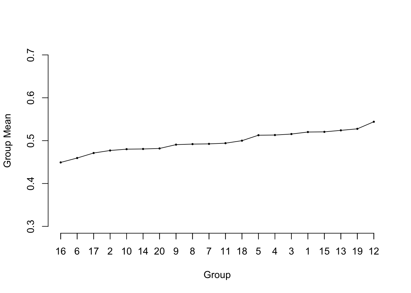
Consider the comparison of 5 groups on a continuous Y. Suppose you observe that two of the groups have a similar mean and the other three also have a similar sample mean. What is wrong with combining the two samples and combining the three samples, then comparing two means? How does this compare to stepwise variable selection?
Name a specific statistical test for which we don’t have a corresponding statistical model
Concerning a multi-group problem or a sequential testing problem what is the frequentist approach to multiplicity correction? The Bayesian approach?

1.1 Hypothesis Testing, Estimation, and Prediction

flowchart LR
uses[Uses of models] --> test[Hypothesis testing]
uses --> estimat[Estimation]
uses --> pred[Prediction]
test --> ftest["Formal tests<br>Formal model<br>comparison<br>(e.g. AIC)"]
estimat --> festimat[Point and interval<br>estimation of one<br>predictor's effect]
pred --> fpred[Estimated outcome<br>or outcome<br>tendency for<br>a subject]

Even when only testing $H_{0}$ a model based approach has advantages:

Permutation and rank tests not as useful for estimation
Cannot readily be extended to cluster sampling or repeated measurements
Models generalize tests
- 2-sample $t$-test, ANOVA $\rightarrow$
  multiple linear regression
- paired $t$-test $\rightarrow$
  linear regression with fixed effects for subjects (block on subjects); linear mixed model with random per-subject intercepts
- Wilcoxon, Kruskal-Wallis, Spearman $\rightarrow$
  proportional odds (PO) ordinal logistic model
- Wilcoxon signed-rank test $\rightarrow$
  replace with rank-difference test $\rightarrow$
  PO model blocking on subject; ordinal mixed model
- log-rank $\rightarrow$ Cox
- See Common statistical tests are linear models by JK Lindeløv
Models not only allow for multiplicity adjustment but for shrinkage of estimates
- Statisticians comfortable with $P$-value adjustment but fail to recognize that the difference between the most different treatments is badly biased

Statistical estimation is usually model-based

Relative effect of increasing cholesterol from 200 to 250 mg/dl on hazard of death, holding other risk factors constant
Adjustment depends on how other risk factors relate to hazard
Usually interested in adjusted (partial) effects, not unadjusted (marginal or crude) effects

1.1.1 Quality of Estimates

Point estimates in the non-Bayesian context
- Bayesian inference does not normally use point estimates but rather entire uncertainty distributions
Parameter being estimated: $\theta$
Estimate: $\hat{\theta}$
Long-term average of $\hat{\theta} : \theta^*$
Bias: $\theta^{*} - \theta$
Variance: long-term average of $(\hat{\theta} - \theta^{*}) ^ 2$
Care most about mean squared error = bias$^{2}$ + variance = long term average of $(\hat{\theta} - \theta) ^ 2$
Other important measures
- Mean absolute error: average $|\hat{\theta} - \theta|$
- Median absolute error: median $|\hat{\theta} - \theta|$
Also of interested: integrated (over diverse observations) MSE etc.
Example: including all possible interactions in a model will minimize bias but have awful MSE

1.3 Misunderstandings about Prediction vs. Classification

flowchart LR
goal[Goal] --> predest[Estimation or Prediction]
goal --> classif[Classification]
predest --> whatpre[Continuous output<br><br>Handles close<br>calls and<br>gray zones<br><br>Provides input to<br>decision maker]
classif --> whatclass[Categorical output<br><br>Hides close calls<br><br>Makes premature<br>decisions<br><br>Does not provide<br>sufficient input<br>to decision maker<br><br>Useful for quick<br>easy decisions or<br>when outcome<br>probabilities are<br>near 0 and 1]

Many analysts desire to develop “classifiers” instead of predictions
Outside of, for example, visual or sound pattern recognition, classification represents a premature decision
See this blog for details
Suppose that

response variable is binary
the two levels represent a sharp dichotomy with no gray zone (e.g., complete success vs. total failure with no possibility of a partial success)
one is forced to assign (classify) future observations to only these two choices
the cost of misclassification is the same for every future observation, and the ratio of the cost of a false positive to the cost of a false negative equals the (often hidden) ratio implied by the analyst’s classification rule

Then classification is still sub-optimal for driving the development of a predictive instrument as well as for hypothesis testing and estimation
Classification and its associated classification accuracy measure—the proportion classified “correctly”—are very sensitive to the relative frequencies of the outcome variable. If a classifier is applied to another dataset with a different outcome prevalence, the classifier may no longer apply.
Far better is to use the full information in the data to develop a probability model, then develop classification rules on the basis of estimated probabilities
- $\uparrow$ power, $\uparrow$ precision, $\uparrow$ decision making
Classification is more problematic if response variable is ordinal or continuous or the groups are not truly distinct (e.g., disease or no disease when severity of disease is actually on a continuum); dichotomizing it up front for the analysis is not appropriate
- minimum loss of information (when dichotomization is at the median) is large
- may require the sample size to increase many–fold to compensate for loss of information Fedorov et al. (2009)
Two-group classification represents artificial forced choice
- best option may be “no choice, get more data”
Unlike prediction (e.g., of absolute risk), classification implicitly uses utility (loss; cost of false positive or false negative) functions
Hidden problems:
- Utility function depends on variables not collected (subjects’ preferences) that are available only at the decision point
- Assumes every subject has the same utility function
- Assumes this function coincides with the analyst’s
Formal decision analysis uses
- optimum predictions using all available data
- subject-specific utilities, which are often based on variables not predictive of the outcome
ROC analysis is misleading except for the special case of mass one-time group decision making with unknowable utilities¹

¹ To make an optimal decision you need to know all relevant data about an individual (used to estimate the probability of an outcome), and the utility (cost, loss function) of making each decision. Sensitivity and specificity do not provide this information. For example, if one estimated that the probability of a disease given age, sex, and symptoms is 0.1 and the “cost” of a false positive equaled the “cost” of a false negative, one would act as if the person does not have the disease. Given other utilities, one would make different decisions. If the utilities are unknown, one gives the best estimate of the probability of the outcome to the decision maker and let them incorporate their own unspoken utilities in making an optimum decision for them.

Besides the fact that cutoffs do not apply to individuals, only to groups, individual decision making does not utilize sensitivity and specificity. For an individual we can compute $\textrm{Prob}(Y=1 | X=x)$; we don’t care about $\textrm{Prob}(Y=1 | X>c)$, and an individual having $X=x$ would be quite puzzled if they were given $\textrm{Prob}(X>c | \textrm{future unknown Y})$ when they already knows $X=x$ so $X$ is no longer a random variable.

Even when group decision making is needed, sensitivity and specificity can be bypassed. For mass marketing, for example, one can rank order individuals by the estimated probability of buying the product, to create a lift curve. This is then used to target the $k$ most likely buyers where $k$ is chosen to meet total program cost constraints.

See Vickers (2008), Briggs & Zaretzki (2008), Gail & Pfeiffer (2005), Bordley (2007), Fan & Levine (2007), Gneiting & Raftery (2007).

Accuracy score used to drive model building should be a continuous score that utilizes all of the information in the data.

In summary:

Classification is a forced choice — a decision.
Decisions require knowledge of the cost or utility of making an incorrect decision.
Predictions are made without knowledge of utilities.
A prediction can lead to better decisions than classification. For example suppose that one has an estimate of the risk of an event, $\hat{P}$. One might make a decision if $\hat{P} < 0.10$ or $\hat{P} > 0.90$ in some situations, even without knowledge of utilities. If on the other hand $\hat{P} = 0.6$ or the confidence interval for $P$ is wide, one might
- make no decision and instead opt to collect more data
- make a tentative decision that is revisited later
- make a decision using other considerations such as the infusion of new resources that allow targeting a larger number of potential customers in a marketing campaign

The Dichotomizing Motorist

The speed limit is 60.
I am going faster than the speed limit.
Will I be caught?

An answer by a dichotomizer:

Are you going faster than 70?

An answer from a better dichotomizer:

If you are among other cars, are you going faster than 73?
If you are exposed are your going faster than 67?

Better:

How fast are you going and are you exposed?

Analogy to most medical diagnosis research in which +/- diagnosis is a false dichotomy of an underlying disease severity:

The speed limit is moderately high.
I am going fairly fast.
Will I be caught?

1.6 Model uncertainty / Data-driven Model Specification

flowchart LR
ms[Model Selection] --> pre[Pre-specified] --> eps[Try to specify<br>a model flexible<br>enough to fit<br><br>Fit assumed<br>to be adequate<br><br>Need not be perfect<br>but as good as<br>any model not<br>requiring larger N] --> nomu[No model<br>uncertainty,<br>accurate statistical<br>inference]
ms --> bayes[Pre-specified<br>Bayesian model<br>with parameters<br>capturing departures<br>from simplicity] --> bac[No binary model<br>choices required] --> api[Accurate posterior<br>inference<br><br>Robust<br><br>Insights about<br>non-normality etc.]
ms --> cont[Contest between<br>desired and<br>more general model] --> pair[Check if more<br>general model is<br>better for the money] --> mmu[Better way to<br>check goodness<br>of fit<br><br>Minimal model<br>uncertainty]
ms --> emp[Empirical] --> gof[Goodness-of-fit<br>checking if<br>involves >2<br> pre-specified<br>models] --> dist
emp --> empus[May be highly<br>unstable if<br>entertain many<br>models or do<br>feature<br>selection] --> dist[Distorted statistical<br>inference]
ms --> ml[Machine learning] --> mluns[May be highly<br>unstable<br>unless N huge] --> noinf[No statistical inference]

Standard errors, C.L., $P$-values, $R^2$ wrong if computed as if the model pre-specified
Stepwise variable selection is widely used and abused
Bootstrap can be used to repeat all analysis steps to properly penalize variances, etc.
Ye (1998): “generalized degrees of freedom” (GDF) for any “data mining” or model selection procedure based on least squares
- Example: 20 candidate predictors, $n=22$, forward stepwise, best 5-variable model: GDF=14.1
- Example: CART, 10 candidate predictors, $n=100$, 19 nodes: GDF=76
See Luo et al. (2006) for an approach involving adding noise to $Y$ to improve variable selection
Another example: $t$-test to compare two means
- Basic test assumes equal variance and normal data distribution
- Typically examine the two sample distributions to decide whether to transform $Y$ or switch to a different test
- Examine the two SDs to decide whether to use the standard test or switch to a Welch $t$-test
- Final confidence interval for mean difference is conditional on the final choices being correct
- Ignores model uncertainty
- Confidence interval will not have the claimed coverage
- Get proper coverage by adding parameters for what you don’t know
  - Bayesian $t$-test: parameters for variance ratio and for d.f. of a $t$-distribution for the raw data (allows heavy tails)

1.6.1 Model Uncertainty and Model Checking

As the Bayesian $t$-test exemplifies, there are advantages of a continuous approach to modeling instead of engaging in dichotomous goodness-of-fit (GOF) assessments. Some general comments:

In a frequentist setting, GOF checking can inflate type I assertion probability $\alpha$ and make confidence intervals falsely narrow. In a Bayesian setting, posterior distributions and resulting uncertainty intervals can be too narrow.
Rather than accepting or not accepting a proposed model on the basis of a GOF assessment, embed the proposed model inside a more general model that relaxes the assumptions, and use AIC or a formal test to decide between the two. Comparing only two pre-specified models will result in minimal model uncertainty. It is often more useful to think of GOF as a contest between the proposed model and a more general model. If the more general model is the most general one that the effective sample size will support, it doesn’t do any good to worry about the adequacy of the more general model.
- More general model could include nonlinear terms and interactions
- It could also relax distributional assumptions, as done with the non-normality parameter in the Bayesian $t$-test
- Often the sample size is not large enough to allow model assumptions to be relaxed without overfitting; AIC assesses whether additional complexities are “good for the money”. If a more complex model results in worse predictions due to overfitting, it is doubtful that such a model should be used for inference.
Instead of focusing on model assumption checking, focus on the impact of making those assumptions, using for example comparison of adjusted $R^2$ measures and bootstrap confidence intervals for differences in predicted values from two models.
In many situations you can use a semiparametric model that makes many fewer assumptions than a parametric model
See this for more in-depth discussion

2.4 Relaxing Linearity Assumption for Continuous Predictors

2.4.1 Avoiding Categorization

Natura non facit saltus
(Nature does not make jumps)
— Gottfried Wilhelm Leibniz

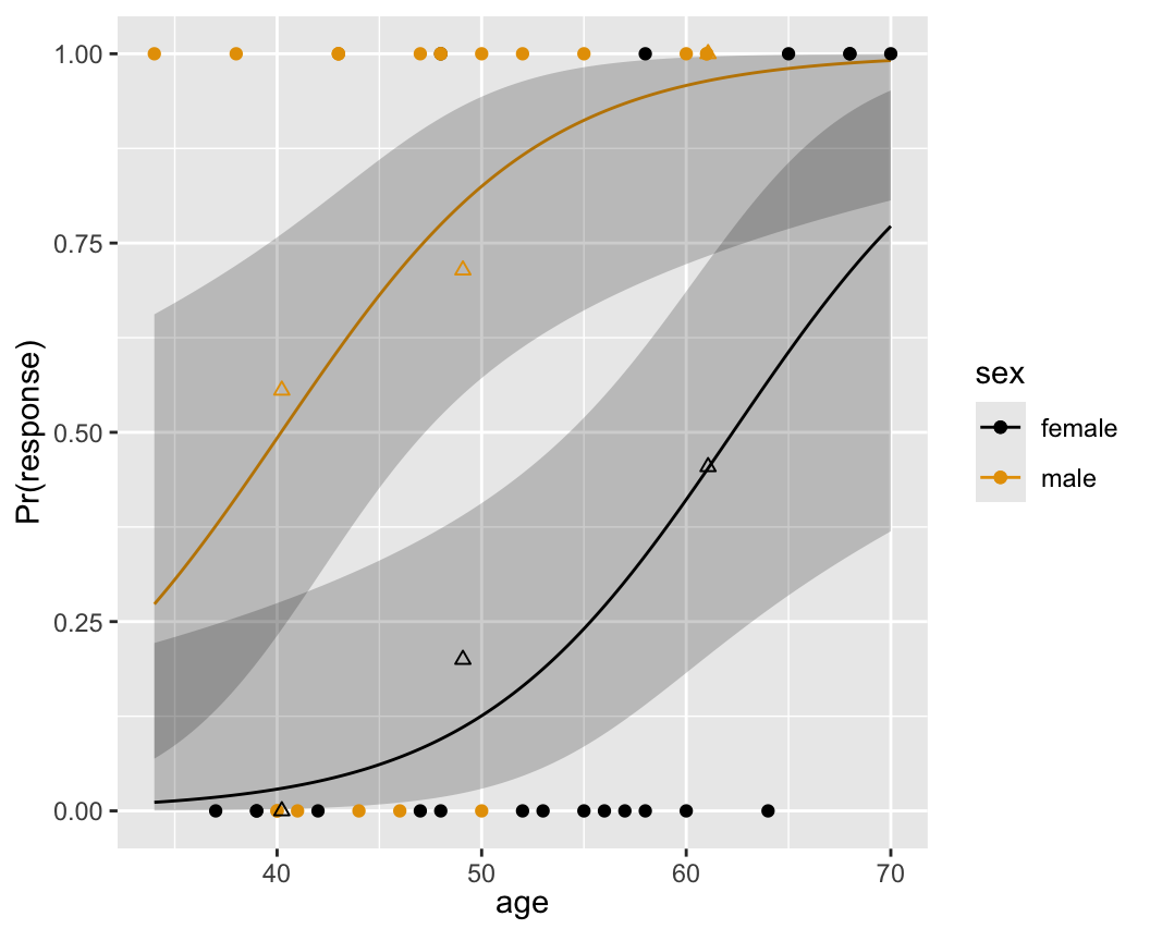
Lucy D’Agostino McGowan

Relationships seldom linear except when predicting one variable from itself measured earlier
Categorizing continuous predictors into intervals is a disaster; see Royston et al. (2006), Altman (1991), Hilsenbeck & Clark (1996), Lausen & Schumacher (1996), Altman et al. (1994), Belcher (1992), Faraggi & Simon (1996), Ragland (1992), Suissa & Blais (1995), Buettner et al. (1997), Maxwell & Delaney (1993), Schulgen et al. (1994), Altman (1998), Holländer et al. (2004), Moser & Coombs (2004), Wainer (2006), Fedorov et al. (2009), Giannoni et al. (2014), Collins et al. (2016), Bennette & Vickers (2012) and Biostatistics for Biomedical Research, Chapter 18.
Some problems caused by this approach:

Estimated values have reduced precision, and associated tests have reduced power
Categorization assumes relationship between predictor and response is flat within intervals; far less reasonable than a linearity assumption in most cases
To make a continuous predictor be more accurately modeled when categorization is used, multiple intervals are required
Because of sample size limitations in the very low and very high range of the variable, the outer intervals (e.g., outer quintiles) will be wide, resulting in significant heterogeneity of subjects within those intervals, and residual confounding
Categorization assumes that there is a discontinuity in response as interval boundaries are crossed. Other than the effect of time (e.g., an instant stock price drop after bad news), there are very few examples in which such discontinuities have been shown to exist.
Categorization only appears to yield interpretable estimates. E.g. odds ratio for stroke for persons with a systolic blood pressure $> 160$ mmHg compared to persons with a blood pressure $\leq 160$ mmHg $\rightarrow$ interpretation of OR depends on distribution of blood pressures in the sample (the proportion of subjects $> 170$, $> 180$, etc.). If blood pressure is modeled as a continuous variable (e.g., using a regression spline, quadratic, or linear effect) one can estimate the ratio of odds for exact settings of the predictor, e.g., the odds ratio for 200 mmHg compared to 120 mmHg.
Categorization does not condition on full information. When, for example, the risk of stroke is being assessed for a new subject with a known blood pressure (say 162~mmHg), the subject does not report to her physician “my blood pressure exceeds 160” but rather reports 162 mmHg. The risk for this subject will be much lower than that of a subject with a blood pressure of 200 mmHg.
If cutpoints are determined in a way that is not blinded to the response variable, calculation of $P$-values and confidence intervals requires special simulation techniques; ordinary inferential methods are completely invalid. E.g.: cutpoints chosen by trial and error utilizing $Y$, even informally $\rightarrow$ $P$-values too small and CLs not accurate³.
Categorization not blinded to $Y$ $\rightarrow$ biased effect estimates (Altman et al. (1994), Schulgen et al. (1994))
“Optimal” cutpoints do not replicate over studies. Holländer et al. (2004) state that “… the optimal cutpoint approach has disadvantages. One of these is that in almost every study where this method is applied, another cutpoint will emerge. This makes comparisons across studies extremely difficult or even impossible. Altman et al. point out this problem for studies of the prognostic relevance of the S-phase fraction in breast cancer published in the literature. They identified 19 different cutpoints used in the literature; some of them were solely used because they emerged as the ‘optimal’ cutpoint in a specific data set. In a meta-analysis on the relationship between cathepsin-D content and disease-free survival in node-negative breast cancer patients, 12 studies were in included with 12 different cutpoints Interestingly, neither cathepsin-D nor the S-phase fraction are recommended to be used as prognostic markers in breast cancer in the recent update of the American Society of Clinical Oncology.” Giannoni et al. (2014) demonstrated that many claimed “optimal cutpoints” are just the observed median values in the sample, which happens to optimize statistical power for detecting a separation in outcomes.
Disagreements in cutpoints (which are bound to happen whenever one searches for things that do not exist) cause severe interpretation problems. One study may provide an odds ratio for comparing body mass index (BMI) $> 30$ with BMI $\leq 30$, another for comparing BMI $> 28$ with BMI $\leq 28$. Neither of these has a good definition and the two estimates are not comparable.
Cutpoints are arbitrary and manipulable; cutpoints can be found that can result in both positive and negative associations Wainer (2006).
If a confounder is adjusted for by categorization, there will be residual confounding that can be explained away by inclusion of the continuous form of the predictor in the model in addition to the categories.

³ If a cutpoint is chosen that minimizes the $P$-value and the resulting $P$-value is 0.05, the true type I error can easily be above 0.5 Holländer et al. (2004).

To summarize: The use of a (single) cutpoint $c$ makes many assumptions, including:

Relationship between $X$ and $Y$ is discontinuous at $X=c$ and only $X=c$
$c$ is correctly found as the cutpoint
$X$ vs. $Y$ is flat to the left of $c$
$X$ vs. $Y$ is flat to the right of $c$
The choice of $c$ does not depend on the values of other predictors

Interactive demonstration of power loss of categorization vs. straight line and quadratic fits in OLS, with varying degree of nonlinearity and noise added to $X$ (must run in RStudio)

Interactive demonstration of lack of fit after categorization of a continuous predictor, and comparison with spline fits, by Stefan Hansen

Code

require(Hmisc)
# Install the manipulate package to make catgNoise work
getRs('catgNoise.r')

Example⁴ of misleading results from creating intervals (here, deciles) of a continuous predictor. Final interval is extremely heterogeneous and is greatly influenced by very large glycohemoglobin values, creating the false impression of an inflection point at 5.9.

⁴ From NHANES III; Diabetes Care 32:1327-34; 2009 adapted from Diabetes Care 20:1183-1197; 1997.

See this for excellent graphical examples of the harm of categorizing predictors, especially when using quantile groups.

2.4.2 Simple Nonlinear Terms

\[C(Y|X_{1}) = \beta_{0}+\beta_{1} X_{1}+\beta_{2} X_{1}^{2} .\]

$H_{0}:$ model is linear in $X_{1}$ vs. $H_{a}:$ model is quadratic in $X_{1} \equiv H_{0}: \beta_{2}=0$.
Test of linearity may be powerful if true model is not extremely non-parabolic
Predictions not accurate in general as many phenomena are non-quadratic
Can get more flexible fits by adding powers higher than 2
But polynomials do not adequately fit logarithmic functions or “threshold” effects, and have unwanted peaks and valleys.

2.4.3 Splines for Estimating Shape of Regression Function and Determining Predictor Transformations

Draftsman’s spline: flexible strip of metal or rubber used to trace curves.
Spline Function: piecewise polynomial
Linear Spline Function: piecewise linear function
- Bi-linear regression: model is $\beta_{0}+\beta_{1}X$ if $X \leq a$, $\beta_{2}+\beta_{3}X$ if $X > a$.
- Problem with this notation: two lines not constrained to join
- To force simple continuity: $\beta_{0} + \beta_{1}X + \beta_{2}(X-a)\times [X>a] = \beta_{0} + \beta_{1}X_{1} + \beta_{2}X_{2}$,
  where $X_{2} = (X_{1}-a) \times [X_{1} > a]$.
- Slope is $\beta_{1}, X \leq a$, $\beta_{1}+\beta_{2}, X > a$.
- $\beta_{2}$ is the slope increment as you pass $a$

See this for a nice review and information about resources in R.

More generally: $x$-axis divided into intervals with endpoints $a,b,c$ (knots).

\[\begin{array}{ccc} f(X) &=& \beta_{0}+\beta_{1}X+\beta_{2}(X-a)_{+}+\beta_{3}(X-b)_{+} \nonumber\\ &+& \beta_{4}(X-c)_{+} , \end{array}\]

where

\[\begin{array}{ccc} (u)_{+}=&u,&u>0 ,\nonumber\\ &0,&u\leq0 . \end{array}\]

\[\begin{array}{ccc} f(X) & = \beta_{0}+\beta_{1}X, & X\leq a \nonumber \\ & = \beta_{0}+\beta_{1}X+\beta_{2}(X-a) & a<X\leq b \\ & = \beta_{0}+\beta_{1}X+\beta_{2}(X-a)+\beta_{3}(X-b) & b<X\leq c \nonumber\\ & = \beta_{0}+\beta_{1}X+\beta_{2}(X-a) & \nonumber\\ & + \beta_{3}(X-b)+\beta_{4}(X-c) & c<X. \nonumber \end{array}\]

Figure 2.1: A linear spline function with knots at $a = 1, b = 3, c = 5$.

\[C(Y|X) = f(X) = X\beta,\] where $X\beta = \beta_{0}+\beta_{1} X_{1}+\beta_{2} X_{2}+\beta_{3}X_{3}+\beta_{4} X_{4}$, and

\[\begin{array}{cc} X_{1}=X & X_{2} = (X-a)_{+}\nonumber\\ X_{3}=(X-b)_{+} & X_{4} = (X-c)_{+} . \end{array}\]

Overall linearity in $X$ can be tested by testing $H_{0} : \beta_{2} = \beta_{3} = \beta_{4} = 0$.

2.4.4 Cubic Spline Functions

Cubic splines are smooth at knots (function, first and second derivatives agree) — can’t see joins.

\[\begin{array}{ccc} f(X) &=& \beta_{0}+\beta_{1}X+\beta_{2}X^{2}+\beta_{3}X^{3}\nonumber\\ &+&\beta_{4}(X-a)_{+}^{3}+ \beta_{5}(X-b)_{+}^{3}+\beta_{6}(X-c)_{+}^{3}\\ &=& X\beta\nonumber \end{array}\] \[\begin{array}{cc} X_{1}=X & X_{2}=X^{2}\nonumber\\ X_{3}=X^{3} & X_{4}=(X-a)_{+}^{3}\\ X_{5}=(X-b)_{+}^{3} & X_{6}=(X-c)_{+}^{3}\nonumber . \end{array}\]

$k$ knots $\rightarrow k+3$ coefficients excluding intercept.

$X^2$ and $X^3$ terms must be included to allow nonlinearity when $X < a$.

stats.stackexchange.com/questions/421964 has some useful descriptions of what happens at the knots, e.g.:

Knots are where different cubic polynomials are joined, and cubic splines force there to be three levels of continuity (the function, its slope, and its acceleration or second derivative (slope of the slope) do not change) at these points. At the knots the jolt (third derivative or rate of change of acceleration) is allowed to change suddenly, meaning the jolt is allowed to be discontinuous at the knots. Between knots, jolt is constant.

The following graphs show the function and its first three derivatives (all further derivatives are zero) for the function given by $f(x) = x + x^{2} + 2x^{3} + 10(x - 0.25)^{3}_{+} - 50(x - 0.5)^{3}_{+} -100(x - 0.75)^{3}_{+}$ for $x$ going from 0 to 1, where there are three knots, at $x=0.25, 0.5, 0.75$.

Code

spar(bty='l', mfrow=c(4,1), bot=-1.5)
x  <- seq(0, 1, length=500)
x1 <- pmax(x - .25, 0)
x2 <- pmax(x - .50, 0)
x3 <- pmax(x - .75, 0)
b1 <- 1; b2 <- 1; b3 <- 2; b4 <- 10; b5 <- -50; b6 <- -100
y  <- b1 * x + b2 * x^2 + b3 * x^3 + b4 * x1^3 + b5 * x2^3 + b6 * x3^3
y1 <- b1     + 2*b2*x   + 3*b3*x^2 + 3*b4*x1^2 + 3*b5*x2^2 + 3*b6*x3^2
y2 <-          2*b2     + 6*b3*x   + 6*b4*x1   + 6*b5*x2   + 6*b6*x3
y3 <-                     6*b3     + 6*b4*(x1>0)+ 6*b5*(x2>0) + 6*b6*(x3>0)

g <- function() abline(v=(1:3)/4, col=gray(.85))
plot(x, y, type='l', ylab=''); g()
text(0, 1.5, 'Function', adj=0)

plot(x, y1, type='l', ylab=''); g()
text(0, -15, 'First Derivative: Slope\nRate of Change of Function',
     adj=0)
plot(x, y2, type='l', ylab=''); g()
text(0, -125, 'Second Derivative: Acceleration\nRate of Change of Slope',
     adj=0)
plot(x, y3, type='l', ylab=''); g()
text(0, -400, 'Third Derivative: Jolt\nRate of Change of Acceleration',
     adj=0)

Figure 2.2: A regular cubic spline function with three levels of continuity that prevent the human eye from detecting the knots. Also shown is the function’s first three derivatives. Knots are located at $x=0.25, 0.5, 0.75$. For $x$ beyond the outer knots, the function is not restricted to be linear. Linearity would imply an acceleration of zero. Vertical lines are drawn at the knots.

2.4.5 Restricted Cubic Splines

Stone & Koo (1985): cubic splines poorly behaved in tails. Constrain function to be linear in tails.
$k+3 \rightarrow k-1$ parameters Devlin & Weeks (1986).

To force linearity when $X < a$: $X^2$ and $X^3$ terms must be omitted
To force linearity when $X$ is beyond the last knot: last two $\beta$ s are redundant, i.e., are just combinations of the other $\beta$ s.

The restricted spline function with $k$ knots $t_{1}, \ldots, t_{k}$ is given by Devlin & Weeks (1986) \[f(X) = \beta_{0}+\beta_{1} X_{1}+\beta_{2} X_{2}+\ldots+\beta_{k-1} X_{k-1},\] where $X_{1} = X$ and for $j=1, \ldots, k-2$,

\[\begin{array}{ccc} X_{j+1} &= &(X-t_{j})_{+}^{3}-(X-t_{k-1})_{+}^{3} (t_{k}-t_{j})/(t_{k}-t_{k-1})\nonumber\\ &+&(X-t_{k})_{+}^{3} (t_{k-1}-t_{j})/(t_{k}-t_{k-1}). \end{array} \tag{2.1}\]

$X_{j}$ is linear in $X$ for $X\geq t_{k}$.

For numerical behavior and to put all basis functions for $X$ on the same scale, R Hmisc and rms package functions by default divide the terms above by $\tau = (t_{k} - t_{1})^{2}$.

Code

require(Hmisc)
spar(mfrow=c(1,2), left=-2)
x <- rcspline.eval(seq(0,1,.01),
                   knots=seq(.05,.95,length=5), inclx=T)
xm <- x
xm[xm > .0106] <- NA
matplot(x[,1], xm, type="l", ylim=c(0,.01),
        xlab=expression(X), ylab='', lty=1)
matplot(x[,1], x,  type="l",
        xlab=expression(X), ylab='', lty=1)

Figure 2.3: Restricted cubic spline component variables for $k = 5$ and knots at $X = .05, .275, .5, .725$, and $.95$. Nonlinear basis functions are scaled by $\tau$. The left panel is a $y$–magnification of the right panel. Fitted functions such as those in Figure 2.4 will be linear combinations of these basis functions as long as knots are at the same locations used here.

Code

spar(left=-2, bot=2, mfrow=c(2,2), ps=13)
x <- seq(0, 1, length=300)
for(nk in 3:6) {
  set.seed(nk)
  knots <- seq(.05, .95, length=nk)
  xx <- rcspline.eval(x, knots=knots, inclx=T)
  for(i in 1 : (nk - 1))
    xx[,i] <- (xx[,i] - min(xx[,i])) /
              (max(xx[,i]) - min(xx[,i]))
  for(i in 1 : 20) {
    beta  <- 2*runif(nk-1) - 1
    xbeta <- xx %*% beta + 2 * runif(1) - 1
    xbeta <- (xbeta - min(xbeta)) /
             (max(xbeta) - min(xbeta))
    if(i == 1) {
      plot(x, xbeta, type="l", lty=1,
           xlab=expression(X), ylab='', bty="l")
      title(sub=paste(nk,"knots"), adj=0, cex=.75)
      for(j in 1 : nk)
        arrows(knots[j], .04, knots[j], -.03,
               angle=20, length=.07, lwd=1.5)
    }
    else lines(x, xbeta, col=i)
  }
}

Figure 2.4: Some typical restricted cubic spline functions for $k = 3, 4, 5, 6$. The $y$–axis is $X\beta$. Arrows indicate knots. These curves were derived by randomly choosing values of $\beta$ subject to standard deviations of fitted functions being normalized.

Interactive demonstration of linear and cubic spline fitting, plus ordinary $4^{th}$ order polynomial. This can be run with RStudio or in an ordinary R session.

Code

require(Hmisc)
getRs('demoSpline.r', put='rstudio')  # to see code in RStudio window
getRs('demoSpline.r')                 # to just run the code

Paul Lambert’s excellent self-contained interactive demonstrations of continuity restrictions, cubic polynomial, linear spline, cubic spline, and restricted cubic spline fitting is at pclambert.net/interactive_graphs. Jordan Gauthier has another nice interactive demonstration at drjgauthier.shinyapps.io/spliny.

See also the excellent resources from Michael Clark here and here and the excellent tutorial by Danielle Navarro here.

Once $\beta_{0}, \ldots, \beta_{k-1}$ are estimated, the restricted cubic spline can be restated in the form

\[\begin{array}{ccc} f(X) &=& \beta_{0}+\beta_{1}X+\beta_{2}(X-t_{1})_{+}^{3}+\beta_{3}(X-t_{2})_{+}^{3}\nonumber\\ && +\ldots+ \beta_{k+1}(X-t_{k})_{+}^{3} \end{array} \tag{2.2}\]

by dividing $\beta_{2},\ldots,\beta_{k-1}$ by $\tau$ and computing

\[\begin{array}{ccc} \beta_{k} &=& [\beta_{2}(t_{1}-t_{k})+\beta_{3}(t_{2}-t_{k})+\ldots\nonumber\\ && +\beta_{k-1}(t_{k-2}-t_{k})]/(t_{k}-t_{k-1})\nonumber\\ \beta_{k+1} &= & [\beta_{2}(t_{1}-t_{k-1})+\beta_{3}(t_{2}-t_{k-1})+\ldots\\ && + \beta_{k-1}(t_{k-2}-t_{k-1})]/(t_{k-1}-t_{k})\nonumber . \end{array}\]

A test of linearity in X can be obtained by testing

\[H_{0} : \beta_{2} = \beta_{3} = \ldots = \beta_{k-1} = 0.\]

Example: Selvin et al. (2010)

2.4.6 Choosing Number and Position of Knots

Knots are specified in advance in regression splines
Locations not important in most situations— Stone (1986), Durrleman & Simon (1989)
Place knots where data exist — fixed quantiles of predictor’s marginal distribution
Fit depends more on choice of $k$

k	Quantiles

3			.10	.5	.90
4			.05	.35	.65	.95
5		.05	.275	.5	.725	.95
6	.05	.23	.41	.59	.77	.95
7	.025	.1833	.3417	.5	.6583	.8167	.975

$n<100$ – replace outer quantiles with 5th smallest and 5th largest $X$ (Stone & Koo (1985)).

Choice of $k$:

Flexibility of fit vs. $n$ and variance
Usually $k=3,4,5$. Often $k=4$
Large $n$ (e.g. $n\geq 100$) – $k=5$
Small $n$ ($<30$, say) – $k=3$
Can use Akaike’s information criterion (AIC) (Atkinson (1980), van Houwelingen & le Cessie (1990)) to choose $k$
This chooses $k$ to maximize model likelihood ratio $\chi^{2} - 2k$.

See Govindarajulu et al. (2007) for a comparison of restricted cubic splines, fractional polynomials, and penalized splines.

2.4.7 Nonparametric Regression

Estimate tendency (mean or median) of $Y$ as a function of $X$
Few assumptions
Especially handy when there is a single $X$
Plotted trend line may be the final result of the analysis
Simplest smoother: moving average

$X$:	1	2	3	5	8
$Y$:	2.1	3.8	5.7	11.1	17.2

\[\begin{array}{ccc} \hat{E}(Y | X=2) &=& \frac{2.1+3.8+5.7}{3} \\ \hat{E}(Y | X=\frac{2+3+5}{3}) &=& \frac{3.8+5.7+11.1}{3} \end{array}\]

overlap OK
problem in estimating $E(Y)$ at outer $X$-values
estimates very sensitive to bin width
Moving linear regression far superior to moving avg. (moving flat line)
Cleveland (1979) moving linear regression smoother loess (locally weighted least squares) is the most popular smoother. To estimate central tendency of $Y$ at $X=x$:
- take all the data having $X$ values within a suitable interval about $x$ (default is $\frac{2}{3}$ of the data)
- fit weighted least squares linear regression within this neighborhood
- points near $x$ given the most weight⁵
- points near extremes of interval receive almost no weight
- loess works much better at extremes of $X$ than moving avg.
- provides an estimate at each observed $X$; other estimates obtained by linear interpolation
- outlier rejection algorithm built-in
loess works for binary $Y$ — just turn off outlier detection
Other popular smoother: Friedman’s “super smoother”
For loess or supsmu amount of smoothing can be controlled by analyst
Another alternative: smoothing splines⁶
Smoothers are very useful for estimating trends in residual plots

⁵ Weight here means something different than regression coefficient. It means how much a point is emphasized in developing the regression coefficients.

⁶ These place knots at all the observed data points but penalize coefficient estimates towards smoothness.

2.4.8 Advantages of Regression Splines over Other Methods

Regression splines have several advantages (Harrell et al. (1988)):

Parametric splines can be fitted using any existing regression program
Regression coefficients estimated using standard techniques (ML or least squares), formal tests of no overall association, linearity, and additivity, confidence limits for the estimated regression function are derived by standard theory.
The fitted function directly estimates transformation predictor should receive to yield linearity in $C(Y|X)$.
Even when a simple transformation is obvious, spline function can be used to represent the predictor in the final model (and the d.f. will be correct). Nonparametric methods do not yield a prediction equation.
Extension to non-additive models.
Multi-dimensional nonparametric estimators often require burdensome computations.

2.5 Recursive Partitioning: Tree-Based Models

Breiman et al. (1984): CART (Classification and Regression Trees) — essentially model-free

Method:

Find predictor so that best possible binary split has maximum value of some statistic for comparing 2 groups
Within previously formed subsets, find best predictor and split maximizing criterion in the subset
Proceed in like fashion until $<k$ obs. remain to split
Summarize $Y$ for the terminal node (e.g., mean, modal category)
Prune tree backward until it cross-validates as well as its “apparent” accuracy, or use shrinkage

Advantages/disadvantages of recursive partitioning:

Does not require functional form for predictors
Does not assume additivity — can identify complex interactions
Can deal with missing data flexibly
Interactions detected are frequently spurious
Does not use continuous predictors effectively
Penalty for overfitting in 3 directions
Often tree doesn’t cross-validate optimally unless pruned back very conservatively
Very useful in messy situations or those in which overfitting is not as problematic (confounder adjustment using propensity scores Cook & Goldman (1988); missing value imputation)

See Austin et al. (2010).

2.5.1 New Directions in Predictive Modeling

The approaches recommended in this course are

fitting fully pre-specified models without deletion of “insignificant” predictors
using data reduction methods (masked to $Y$) to reduce the dimensionality of the predictors and then fitting the number of parameters the data’s information content can support
use shrinkage (penalized estimation) to fit a large model without worrying about the sample size.

The data reduction approach can yield very interpretable, stable models, but there are many decisions to be made when using a two-stage (reduction/model fitting) approach, Newer approaches are evolving, including the following. These new approach handle continuous predictors well, unlike recursive partitioning.

lasso (shrinkage using L1 norm favoring zero regression coefficients) - Tibshirani (1996), Steyerberg et al. (2000)
elastic net (combination of L1 and L2 norms that handles the $p > n$ case better than the lasso) Zou & Hastie (2005)
adaptive lasso H. H. Zhang & Lu (2007), H. Wang & Leng (2007)
more flexible lasso to differentially penalize for variable selection and for regression coefficient estimation (Radchenko & James (2008))
group lasso to force selection of all or none of a group of related variables (e.g., indicator variables representing a polytomous predictor)
group lasso-like procedures that also allow for variables within a group to be removed (S. Wang et al. (2009))
sparse-group lasso using L1 and L2 norms to achieve spareness on groups and within groups of variables (N. Simon et al. (2013))
adaptive group lasso (Wang & Leng)
Breiman’s nonnegative garrote (Xiong (2010))
“preconditioning”, i.e., model simplification after developing a “black box” predictive model - Paul et al. (2008),Nott & Leng (2010)
sparse principal components analysis to achieve parsimony in data reduction Witten & Tibshirani (2008),Zhou et al. (2006),Leng & Wang (2009),Lee et al. (2010)
bagging, boosting, and random forests Hastie et al. (2008)

One problem prevents most of these methods from being ready for everyday use: they require scaling predictors before fitting the model. When a predictor is represented by nonlinear basis functions, the scaling recommendations in the literature are not sensible. There are also computational issues and difficulties obtaining hypothesis tests and confidence intervals.

When data reduction is not required, generalized additive models Hastie & Tibshirani (1990), Wood (2006) should also be considered.

2.6 Multiple Degree of Freedom Tests of Association

\[C(Y|X) = \beta_{0}+\beta_{1}X_{1}+\beta_{2}X_{2}+\beta_{3}X_{2}^{2} ,\] $H_{0}: \beta_{2}=\beta_{3}=0$ with 2 d.f. to assess association between $X_{2}$ and outcome.

In the 5-knot restricted cubic spline model \[C(Y|X) = \beta_{0}+\beta_{1}X+\beta_{2}X'+\beta_{3}X''+\beta_{4}X''' ,\] $H_{0}: \beta_{1}=\ldots=\beta_{4}=0$

Test of association: 4 d.f.
Insignificant $\rightarrow$ dangerous to interpret plot
What to do if 4 d.f. test insignificant, 3 d.f. test for linearity insig., 1 d.f. test sig. after delete nonlinear terms?

Grambsch & O’Brien (1991) elegantly described the hazards of pretesting

Studied quadratic regression
Showed 2 d.f. test of association is nearly optimal even when regression is linear if nonlinearity entertained
Considered ordinary regression model
$E(Y|X) =\beta_{0}+\beta_{1}X+\beta_{2}X^{2}$
Two ways to test association between $X$ and $Y$
Fit quadratic model and test for linearity ($H_{0}: \beta_{2}=0$)
$F$-test for linearity significant at $\alpha=0.05$ level $\rightarrow$ report as the final test of association the 2 d.f. $F$ test of $H_{0}: \beta_{1}=\beta_{2}=0$
If the test of linearity insignificant, refit without the quadratic term and final test of association is 1 d.f. test, $H_{0}:\beta_{1}=0 | \beta_{2}=0$
Showed that type I error $> \alpha$
Fairly accurate $P$-value obtained by instead testing against $F$ with 2 d.f. even at second stage
Cause: are retaining the most significant part of $F$
BUT if test against 2 d.f. can only lose power when compared with original $F$ for testing both $\beta$s
$SSR$ from quadratic model $> SSR$ from linear model

2.7 Assessment of Model Fit

2.7.1 Regression Assumptions

The general linear regression model is \[C(Y|X) = X\beta =\beta_{0}+\beta_{1}X_{1}+\beta_{2}X_{2}+\ldots+\beta_{k}X_{k} .\] Verify linearity and additivity. Special case: \[C(Y|X) = \beta_{0}+\beta_{1}X_{1}+\beta_{2}X_{2},\] where $X_{1}$ is binary and $X_{2}$ is continuous.

Figure 2.5: Regression assumptions for one binary and one continuous predictor

Methods for checking fit:

1. Fit simple linear additive model and check examine residual plots for patterns

For OLS: box plots of $e$ stratified by $X_{1}$, scatterplots of $e$ vs. $X_{2}$ and $\hat{Y}$, with trend curves (want flat central tendency, constant variability)
For normality, qqnorm plots of overall and stratified residuals

Advantage: Simplicity

Disadvantages:

Can only compute standard residuals for uncensored continuous response
Subjective judgment of non-randomness
Hard to handle interaction
Hard to see patterns with large $n$ (trend lines help)
Seeing patterns does not lead to corrective action

2. Scatterplot of $Y$ vs. $X_{2}$ using different symbols according to values of $X_{1}$

Advantages: Simplicity, can see interaction

Disadvantages:

Scatterplots cannot be drawn for binary, categorical, or censored $Y$
Patterns difficult to see if relationships are weak or $n$ large

3. Stratify the sample by $X_{1}$ and quantile groups (e.g. deciles) of $X_{2}$; estimate $C(Y|X_{1},X_{2})$ for each stratum

Advantages: Simplicity, can see interactions, handles censored $Y$ (if you are careful)

Disadvantages:

Requires large $n$
Does not use continuous var. effectively (no interpolation)
Subgroup estimates have low precision
Dependent on binning method

4. Separately for levels of $X_{1}$ fit a nonparametric smoother relating $X_{2}$ to $Y$

Advantages: All regression aspects of the model can be summarized efficiently with minimal assumptions

Disadvantages:

Does not apply to censored $Y$
Hard to deal with multiple predictors

5. Fit flexible nonlinear parametric model

Advantages:

One framework for examining the model assumptions, fitting the model, drawing formal inference
d.f. defined and all aspects of statistical inference “work as advertised”

Disadvantages:

Complexity
Generally difficult to allow for interactions when assessing patterns of effects

Confidence limits, formal inference can be problematic for methods 1-4.

Restricted cubic spline works well for method 5.

\[\begin{array}{ccc} \hat{C}(Y|X) &=& \hat{\beta}_{0}+\hat{\beta}_{1}X_{1}+\hat{\beta}_{2}X_{2}+\hat{\beta}_{3}X_{2}'+\hat{\beta}_{4}X_{2}'' \nonumber\\ &=& \hat{\beta}_{0}+\hat{\beta}_{1}X_{1}+\hat{f}(X_{2}) , \end{array}\]

where \[\hat{f}(X_{2}) = \hat{\beta}_{2}X_{2}+\hat{\beta}_{3}X_{2}'+\hat{\beta}_{4}X_{2}'' ,\] $\hat{f}(X_{2})$ spline-estimated transformation of $X_{2}$.

Plot $\hat{f}(X_{2})$ vs. $X_{2}$
$n$ large $\rightarrow$ can fit separate functions by $X_{1}$
Test of linearity: $H_{0}:\beta_{3}=\beta_{4}=0$
Few good reasons to do the test other than to demonstrate that linearity is not a good default assumption
Nonlinear $\rightarrow$ use transformation suggested by spline fit or keep spline terms
Tentative transformation $g(X_{2})$ $\rightarrow$ check adequacy by expanding $g(X_{2})$ in spline function and testing linearity
Can find transformations by plotting $g(X_{2})$ vs. $\hat{f}(X_{2})$ for variety of $g$
Multiple continuous predictors $\rightarrow$ expand each using spline
Example: assess linearity of $X_{2}, X_{3}$

\[\begin{array}{ccc} C(Y|X) &=& \beta_{0}+\beta_{1}X_{1}+\beta_{2}X_{2}+\beta_{3}X_{2}'+\beta_{4}X_{2}'' \nonumber\\ &+& \beta_{5}X_{3}+\beta_{6}X_{3}'+\beta_{7}X_{3}'' , \end{array}\]

Overall test of linearity $H_{0}: \beta_{3}=\beta_{4}=\beta_{6}=\beta_{7}=0$, with 4 d.f.

2.7.2 Modeling and Testing Complex Interactions

Note: Interactions will be misleading if main effects are not properly modeled (M. Zhang et al. (2020)).

Suppose $X_1$ binary or linear, $X_2$ continuous:

\[\begin{array}{ccc} C(Y|X) & = & \beta_{0}+\beta_{1}X_{1}+\beta_{2}X_{2}+\beta_{3}X_{2}'+\beta_{4}X_{2}'' \\ \nonumber &&+\beta_{5}X_{1}X_{2}+\beta_{6}X_{1}X_{2}'+\beta_{7}X_{1}X_{2}'' \end{array}\]

Simultaneous test of linearity and additivity: $H_{0}: \beta_{3} = \ldots = \beta_{7} = 0$.

2 continuous variables: could transform separately and form simple product
But transformations depend on whether interaction terms adjusted for, so it is usually not possible to estimate transformations and interaction effects other than simultaneously
Compromise: Fit interactions of the form $X_{1} f(X_{2})$ and $X_{2} g(X_{1})$:

\[\begin{array}{ccc} C(Y|X) & = & \beta_{0}+\beta_{1}X_{1}+\beta_{2}X_{1}'+\beta_{3}X_{1}'' \nonumber\\ &+& \beta_{4}X_{2}+\beta_{5}X_{2}'+\beta_{6}X_{2}'' \nonumber\\ &+& \beta_{7}X_{1}X_{2}+\beta_{8}X_{1}X_{2}'+\beta_{9}X_{1}X_{2}'' \\ &+& \beta_{10}X_{2}X_{1}'+\beta_{11}X_{2}X_{1}'' \nonumber \end{array} \tag{2.3}\]

Test of additivity is $H_{0}: \beta_{7} = \beta_{8} = \ldots = \beta_{11} = 0$ with 5 d.f.
Test of lack of fit for the simple product interaction with $X_{2}$ is $H_{0}: \beta_{8} = \beta_{9} = 0$
Test of lack of fit for the simple product interaction with $X_{1}$ is $H_{0}: \beta_{10} = \beta_{11} = 0$

General spline surface:

Cover $X_{1} \times X_{2}$ plane with grid and fit patch-wise cubic polynomial in two variables
Restrict to be of form $aX_{1}+bX_{2}+cX_{1}X_{2}$ in corners
Uses all $(k-1)^{2}$ cross-products of restricted cubic spline terms
See Gray (1992), Gray (1994) for penalized splines allowing control of effective degrees of freedom. See Berhane et al. (2008) for a good discussion of tensor splines.

Figure 2.6: Logistic regression estimate of probability of a hemorrhagic stroke for patients in the GUSTO-I trial given $t$-PA, using a tensor spline of two restricted cubic splines and penalization (shrinkage). Dark (cold color) regions are low risk, and bright (hot) regions are higher risk.

Figure 2.6 is particularly interesting because the literature had suggested (based on approximately 24 strokes) that pulse pressure was the main cause of hemorrhagic stroke whereas this flexible modeling approach (based on approximately 230 strokes) suggests that mean arterial blood pressure (roughly a $45^\circ$ line) is what is most important over a broad range of blood pressures. At the far right one can see that pulse pressure (axis perpendicular to $45^\circ$ line) may have an impact although a non-monotonic one.

Other issues:

$Y$ non-censored (especially continuous) $\rightarrow$ multi-dimensional scatterplot smoother (Chambers & Hastie (1992))
Interactions of order $>2$: more trouble
2-way interactions among $p$ predictors: pooled tests
$p$ tests each with $p-1$ d.f.

Some types of interactions to pre-specify in clinical studies:

Treatment $\times$ severity of disease being treated
Age $\times$ risk factors
Age $\times$ type of disease
Measurement $\times$ state of a subject during measurement
Race $\times$ disease
Calendar time $\times$ treatment
Quality $\times$ quantity of a symptom
Measurement $\times$ amount of deterioration of the measurement

The last example is worth expanding as an example in model formulation. Consider the following study.

A sample of patients seen over several years have a blood sample taken at time of hospitalization
Blood samples are frozen
Long after the last patient was sampled, the blood samples are thawed all in the same week and a blood analysis is done
It is known that the quality of the blood analysis deteriorates roughly logarithmically by the age of the sample; blood measurements made on old samples are assumed to be less predictive of outcome
This is reflected in an interaction between a function of sample age and the blood measurement B⁷
Patients were followed for an event, and the outcome variable of interest is the time from hospitalization to that event
To not assume a perfect logarithmic relationship for sample age on the effect of the blood measurement, a restricted cubic spline model with 3 default knots will be fitted for log sample age
Sample age is assumed to not modify the effects of non-blood predictors patient age and sex
Model may be specified the following way using the R rms package to fit a Cox proportional hazards model
Test for nonlinearity of sampleAge tests the adequacy of assuming a plain logarithmic trend in sample age

⁷ For continuous $Y$ one might need to model the residual variance of $Y$ as increasing with sample age, in addition to modeling the mean function.

Code

f <- cph(Surv(etime, event) ~ rcs(log(sampleAge), 3) * rcs(B, 4) +
           rcs(age, 5) * sex, data=mydata)

The B $\times$ sampleAge interaction effects have 6 d.f. and tests whether the sample deterioration affects the effect of B. By not assuming that B has the same effect for old samples as for young samples, the investigator will be able to estimate the effect of B on outcome when the blood analysis is ideal by inserting sampleAge = 1 day when requesting predicted values as a function of B.

2.8 Complex Curve Fitting Example

Restricted cubic spline
Discontinuity (interrupted time series analysis)
Cyclic trend (seasonality)
Data from academic.oup.com/ije/article/46/1/348/2622842 by Bernal et al. (2017)
Rates of hospital admissions for acute coronary events in Sicily before and after a smoking ban on 2005-01
Poisson regression on case counts, adjusted for population size as an offset variable (analyzes event rate) (see stats.stackexchange.com/questions/11182)
Classic interrupted time series puts a discontinuity at the intervention point and assesses statistical evidence for a nonzero jump height
We will do that and also fit a continuous cubic spline but with multiple knots near the intervention point
All in context of long-term and seasonal trends
Uses the rms package gTrans function documented at hbiostat.org/R/rms/gtrans.html
Can do this without gTrans but harder to plot predicted values, get contrasts, and get chunk tests
Time variable is months after 2001-12-01

Code

require(rms)  # engages rms which also engages Hmisc which provides getHdata
options(prType='html')   # applies to printing model fits
getHdata(sicily)   # fetch dataset from hbiostat.org/data
d    <- sicily
dd   <- datadist(d);  options(datadist='dd')

Start with a standard restricted cubic spline fit, 6 knots at default quantile locations. From the fitted Poisson model we estimate the number of cases per a constant population size of 100,000.

Code

require(ggplot2)
g   <- function(x) exp(x) * 100000
off <- list(stdpop=mean(d$stdpop))    # offset for prediction (383464.4)
w   <- geom_point(aes(x=time, y=rate), data=d)
v   <- geom_vline(aes(xintercept=37, col=I('red')))
yl  <- ylab('Acute Coronary Cases Per 100,000')
f   <- Glm(aces ~ offset(log(stdpop)) + rcs(time, 6),
           data=d, family='poisson')
f$aic

[1] 721.5237

Code

ggplot(Predict(f, fun=g, offset=off)) + w + v + yl

To add seasonality to the model can add sine and/or cosine terms
See pmean.com/07/CyclicalTrends.html by Steve Simon
If you knew the month at which incidence is a minimum, could just add a sine term to the model
Adding both sine and cosine terms effectively allows for a model parameter that estimates the time origin
Assume the period (cycle length) is 12m

Code

# Save knot locations
k  <- attr(rcs(d$time, 6), 'parms')
k

[1]  5.00 14.34 24.78 35.22 45.66 55.00

Code

kn <- k
# rcspline.eval is the rcs workhorse
h <- function(x) cbind(rcspline.eval(x, kn),
                       sin=sin(2*pi*x/12), cos=cos(2*pi*x/12))
f <- Glm(aces ~ offset(log(stdpop)) + gTrans(time, h),
         data=d, family='poisson')
f$aic

[1] 674.112

Code

ggplot(Predict(f, fun=g, offset=off)) + w + v + yl

Next add more knots near intervention to allow for sudden change

Code

kn <- sort(c(k, c(36, 37, 38)))
f <- Glm(aces ~ offset(log(stdpop)) + gTrans(time, h),
         data=d, family='poisson')
f$aic

[1] 661.7904

Code

ggplot(Predict(f, fun=g, offset=off)) + w + v + yl

Now make the slow trend simpler (6 knots) but add a discontinuity at the intervention. More finely control times at which predictions are requested, to handle discontinuity.

Code

h <- function(x) {
  z <- cbind(rcspline.eval(x, k),
             sin=sin(2*pi*x/12), cos=cos(2*pi*x/12),
             jump=x >= 37)
  attr(z, 'nonlinear') <- 2 : ncol(z)
  z
    }
f <- Glm(aces ~ offset(log(stdpop)) + gTrans(time, h),
         data=d, family='poisson', x=TRUE, y=TRUE) # x, y for LRTs
f$aic

[1] 659.6044

Code

times <- sort(c(seq(0, 60, length=200), 36.999, 37, 37.001))
ggplot(Predict(f, time=times, fun=g, offset=off)) + w + v + yl

Look at fit statistics especially evidence for the jump

Code

General Linear Model

Glm(formula = aces ~ offset(log(stdpop)) + gTrans(time, h), family = "poisson", 
    data = d, x = TRUE, y = TRUE)

	Model Likelihood Ratio Test
Obs 59	LR χ² 169.64
Residual d.f. 51	d.f. 7
g 0.080	Pr(>χ²) <0.0001

	β	S.E.	Wald Z	Pr(>\|Z\|)
Intercept	-6.2118	0.0095	-656.01	<0.0001
time	0.0635	0.0113	5.63	<0.0001
time'	-0.1912	0.0433	-4.41	<0.0001
time''	0.2653	0.0760	3.49	0.0005
time'''	-0.2409	0.0925	-2.61	0.0092
sin	0.0343	0.0067	5.11	<0.0001
cos	0.0380	0.0065	5.86	<0.0001
jump	-0.1268	0.0313	-4.06	<0.0001

Evidence for an intervention effect (jump)
Evidence for seasonality
Could have analyzed rates using a semiparametric model

Compute likelihood ratio $\chi^2$ test statistics for this model

Code

anova(f, test='LR')

	χ²	d.f.	P
Likelihood Ratio Statistics for `aces`
time	169.64	7	<0.0001
Nonlinear	127.03	6	<0.0001
TOTAL	169.64	7	<0.0001

Get a joint LR test of seasonality and discontinuity by omitting 3 terms from the model

Code

g <- Glm(aces ~ offset(log(stdpop)) + rcs(time, k),
         data=d, family='poisson')
lrtest(f, g)


Model 1: aces ~ offset(log(stdpop)) + gTrans(time, h)
Model 2: aces ~ offset(log(stdpop)) + rcs(time, k)

  L.R. Chisq         d.f.            P 
6.591931e+01 2.000000e+00 4.884981e-15

4 Multivariable Modeling Strategies

Scientific Big Picture

Thanks to Drew Levy for key contributions

Rigorous judgements about information quality and sufficiency for explicit objectives should precede any modeling
- Undertaking modeling and inference and subsequently apologizing for data deficiencies results in scientific noise
Study design and measurement of key variables are $\frac{9}{10}$ of the problem
Distinguish predictive vs. causitive effects of $X$
Is the current sample size large enough to do an analysis whose goal is to find definitive answers that do not need to be independently validated?
- In other words is $N$ large enough to submit a paper where the results of the analysis do not require external validation to be credible and actionable?
- Near futility of analyses with $p > N$
Poor quality data in abundant quantity are readily available
- Data in sufficient quantity and quality are much less available
- High quality data in sufficient quantity are rare
- Be clear-eyed and honest about your data resources
Is $N$ even large enough to do exploratory analyses?
If $N$ is insufficient and you want to proceed, you must replace the unavailable data with assumptions or knowledge to make the effective sample size adequate
- All-or-nothing assumptions (how treatments and humans function, which variables are relevant, which variables have linear effects, which interactions are real, etc.), or
- Informative Bayesian prior distributions
See On the uses and abuses of regression models by JB Carlin and M Moreno-Betancur. See also this.

Modeling Strategy in a Nutshell

“Spending d.f.”: examining or fitting parameters in models, or examining tables or graphs that utilize $Y$ to tell you how to model variables
If wish to preserve statistical properties, can’t retrieve d.f. once they are “spent” (see Grambsch & O’Brien (1991))
If a scatterplot suggests linearity and you fit a linear model, how many d.f. did you actually spend (i.e., the d.f. that when put into a formula results in accurate confidence limits or $P$-values)?

Decide number of d.f. that can be spent
Decide where to spend them
Spend them
General references: (Giudice et al., 2011; Harrell et al., 1996; Nick & Hardin, 1999; Steyerberg et al., 2001)

There are many choices to be made when deciding upon a global modeling strategy, including choice between

parametric and nonparametric procedures
parsimony and complexity
parsimony and good discrimination ability
interpretable models and black boxes.

4.1 Prespecification of Predictor Complexity Without Later Simplification

Rarely expect linearity
Can’t always use graphs or other devices to choose transformation
If select from among many transformations, results biased
Need to allow flexible nonlinearity to potentially strong predictors not known to predict linearly
Once decide a predictor is “in” can choose no. of parameters to devote to it using a general association index with $Y$
Need a measure of “potential predictive punch”
Measure needs to mask analyst to true form of regression to preserve statistical properties

Motivating examples:

Code

# Overfitting a flat relationship
require(rms)
set.seed(1)
x <- runif(1000)
y <- runif(1000, -0.5, 0.5)
dd <- datadist(x, y); options(datadist='dd')
par(mfrow=c(2,2), mar=c(2, 2, 3, 0.5))
pp <- function(actual) {
  yhat  <- predict(f, data.frame(x=xs))
  yreal <- actual(xs)
  plot(0, 0, xlim=c(0,1),
       ylim=range(c(quantile(y, c(0.1, 0.9)), yhat,
                    yreal)),
       type='n', axes=FALSE)
  axis(1, labels=FALSE); axis(2, labels=FALSE)
  lines(xs, yreal)
  lines(xs, yhat, col='blue')
}
f <- ols(y ~ rcs(x, 5))
xs <- seq(0, 1, length=150)
pp(function(x) 0*x)
title('Mild Error:\nOverfitting a Flat Relationship',
      cex=0.5)
y <- x + runif(1000, -0.5, 0.5)
f <- ols(y ~ rcs(x, 5))
pp(function(x) x)
title('Mild Error:\nOverfitting a Linear Relationship',
      cex=0.5)
y <- x^4 + runif(1000, -1, 1)
f <- ols(y ~ x)
pp(function(x) x^4)
title('Serious Error:\nUnderfitting a Steep Relationship',
      cex=0.5)
y <- - (x - 0.5) ^ 2 + runif(1000, -0.2, 0.2)
f <- ols(y ~ x)
pp(function(x) - (x - 0.5) ^ 2)
title('Tragic Error:\nMonotonic Fit to\nNon-Monotonic Relationship',
      cex=0.5)

Figure 4.1: Fitting errors to withstand or to avoid

Examples of Reducing the Number of Parameters
Categorical predictor with $k$ levels	Collapse less frequent categories into “other”
Continuous predictor represented as $k$-knot restricted cubic spline	Reduce $k$ to a number as low as 3, or 0 (linear)

4.1.1 Learning From a Saturated Model

When the effective sample size available is sufficiently large so that a saturated main effects model may be fitted, a good approach to gauging predictive potential is the following.

Let all continuous predictors be represented as restricted cubic splines with $k$ knots, where $k$ is the maximum number of knots the analyst entertains for the current problem.
Let all categorical predictors retain their original categories except for pooling of very low prevalence categories (e.g., ones containing $<6$ observations).
Fit this general main effects model.
Compute the partial $\chi^2$ statistic for testing the association of each predictor with the response, adjusted for all other predictors. In the case of ordinary regression convert partial $F$ statistics to $\chi^2$ statistics or partial $R^2$ values.
Make corrections for chance associations to “level the playing field” for predictors having greatly varying d.f., e.g., subtract the d.f. from the partial $\chi^2$ (the expected value of $\chi^{2}_{p}$ is $p$ under $H_{0}$).
Make certain that tests of nonlinearity are not revealed as this would bias the analyst.
Sort the partial association statistics in descending order.

Commands in the rms package can be used to plot only what is needed. Here is an example for a logistic model.

Code

f <- lrm(y ~ sex + race + rcs(age,5) + rcs(weight,5) +
         rcs(height,5) + rcs(blood.pressure,5))
plot(anova(f))

4.1.2 Using Marginal Generalized Rank Correlations

When collinearities or confounding are not problematic, a quicker approach based on pairwise measures of association can be useful. This approach will not have numerical problems (e.g., singular covariance matrix) and is based on:

2 d.f. generalization of Spearman $\rho$—$R^2$ based on $rank(X)$ and $rank(X)^2$ vs. $rank(Y)$
$\rho^2$ can detect U-shaped relationships
For categorical $X$, $\rho^2$ is $R^2$ from dummy variables regressed against $rank(Y)$; this is tightly related to the Wilcoxon-Mann-Whitney-Kruskal-Wallis rank test for group differences¹
Sort variables by descending order of $\rho^2$
Specify number of knots for continuous $X$, combine infrequent categories of categorical $X$ based on $\rho^2$

¹ This test statistic does not inform the analyst of which groups are different from one another.

Allocating d.f. based on partial tests of association or sorting $\rho^2$ is a fair procedure because

We already decided to keep variable in model no matter what $\rho^2$ or $\chi^2$ values are seen
$\rho^2$ and $\chi^2$ do not reveal degree of nonlinearity; high value may be due solely to strong linear effect
low $\rho^2$ or $\chi^2$ for a categorical variable might lead to collapsing the most disparate categories

Initial simulations show the procedure to be conservative. Note that one can move from simpler to more complex models but not the other way round

4.3 Variable Selection

Series of potential predictors with no prior knowledge
$\uparrow$ exploration $\rightarrow$ $\uparrow$ shrinkage (overfitting)
Summary of problem: $E(\hat{\beta} | \hat{\beta}$ “significant” $) \neq \beta$ (Chatfield, 1995)
Biased $R^2$, $\hat{\beta}$, standard errors, $P$-values too small
$F$ and $\chi^2$ statistics do not have the claimed distribution² (Grambsch & O’Brien, 1991)
Will result in residual confounding if use variable selection to find confounders (Greenland, 2000)
Derksen & Keselman (1992) found that in stepwise analyses the final model represented noise 0.20-0.74 of time, final model usually contained $< \frac{1}{2}$ actual number of authentic predictors. Also:

² Lockhart et al. (2013) provide an example with $n=100$ and 10 orthogonal predictors where all true $\beta$s are zero. The test statistic for the first variable to enter has type I assertion probability of 0.39 when the nominal $\alpha$ is set to 0.05.

The degree of correlation between the predictor variables affected the frequency with which authentic predictor variables found their way into the final model.

The number of candidate predictor variables affected the number of noise variables that gained entry to the model.

The size of the sample was of little practical importance in determining the number of authentic variables contained in the final model.

The population multiple coefficient of determination could be faithfully estimated by adopting a statistic that is adjusted by the total number of candidate predictor variables rather than the number of variables in the final model.

Global test with $p$ d.f. insignificant $\rightarrow$ stop

Simulation experiment, true $\sigma^{2} = 6.25$, 8 candidate variables, 4 of them related to $Y$ in the population. Select best model using all possible subsets regression to maximize $R^{2}_{adj}$ (all possible subsets is not usually recommended but gives variable selection more of a chance to work in this context).

Note: The audio was made using stepAIC with collinearities in predictors. The code below allows for several options. Here we use all possible subsets of predictors and force predictors to be uncorrelated, which is the easiest case for variable selection.

Code

require(MASS)    # provides stepAIC function
require(leaps)   # provides regsubsets function
sim <- function(n, sigma=2.5, method=c('stepaic', 'leaps'),
                pr=FALSE, prcor=FALSE, dataonly=FALSE) {
  method <- match.arg(method)
  if(uncorrelated) {
    x1 <- rnorm(n)
    x2 <- rnorm(n)
    x3 <- rnorm(n)
    x4 <- rnorm(n)
    x5 <- rnorm(n)
    x6 <- rnorm(n)
    x7 <- rnorm(n)
    x8 <- rnorm(n)
    }
  else {
      x1 <- rnorm(n)
      x2 <- x1 + 2.0 * rnorm(n)       # was + 0.5 * rnorm(n)
      x3 <- rnorm(n)
      x4 <- x3 + 1.5 * rnorm(n)
      x5 <- x1 + rnorm(n)/1.3
      x6 <- x2 + 2.25 * rnorm(n)      # was rnorm(n)/1.3
      x7 <- x3 + x4 + 2.5 * rnorm(n)  # was + rnorm(n)
      x8 <- x7 + 4.0 * rnorm(n)       # was + 0.5 * rnorm(n)
  }
  z <- cbind(x1,x2,x3,x4,x5,x6,x7,x8)
  if(prcor) return(round(cor(z), 2))
  lp <- x1 + x2 + .5*x3 + .4*x7
  y <- lp + sigma*rnorm(n)
  if(dataonly) return(list(x=z, y=y))
  if(method == 'leaps') {
    s     <- summary(regsubsets(z, y))
    best  <- which.max(s$adjr2)
    xvars <- s$which[best, -1]   # remove intercept
    ssr   <- s$rss[best]
    p     <- sum(xvars)
    xs    <- if(p == 0) 'none' else paste((1 : 8)[xvars], collapse='')
    if(pr) print(xs)
    ssesw <- (n - 1) * var(y) - ssr
    s2s   <- ssesw / (n - p - 1)
    yhat  <- if(p == 0) mean(y) else fitted(lm(y ~ z[, xvars]))
  }
  f <- lm(y ~ x1 + x2 + x3 + x4 + x5 + x6 + x7 + x8)
  if(method == 'stepaic') {
    g <- stepAIC(f, trace=0)
    p <- g$rank - 1
    xs <- if(p == 0) 'none' else
      gsub('[ <br>+x]','', as.character(formula(g))[3])
    if(pr) print(formula(g), showEnv=FALSE)
    ssesw <- sum(resid(g)^2)
    s2s   <- ssesw/g$df.residual
    yhat  <- fitted(g)
  }
  # Set SSEsw / (n - gdf - 1) = true sigma^2
  gdf <- n - 1 - ssesw / (sigma^2)
  # Compute root mean squared error against true linear predictor
  rmse.full <- sqrt(mean((fitted(f) - lp) ^ 2))
  rmse.step <- sqrt(mean((yhat - lp) ^ 2))
  list(stats=c(n=n, vratio=s2s/(sigma^2),
         gdf=gdf, apparentdf=p, rmse.full=rmse.full, rmse.step=rmse.step),
       xselected=xs)
}

rsim <- function(B, n, method=c('stepaic', 'leaps')) {
  method <- match.arg(method)
  xs <- character(B)
  r <- matrix(NA, nrow=B, ncol=6)
  for(i in 1:B) {
    w     <- sim(n, method=method)
    r[i,] <- w$stats
    xs[i] <- w$xselected
  }
  colnames(r) <- names(w$stats)
  s <- apply(r, 2, median)
  p <- r[, 'apparentdf']
  s['apparentdf'] <- mean(p)
  print(round(s, 2))
  print(table(p))
  cat('Prob[correct model]=', round(sum(xs == '1237')/B, 2), '\n')
}

Show the correlation matrix being assumed for the $X$s:

Code

uncorrelated <- TRUE
sim(50000, prcor=TRUE)

      x1   x2    x3   x4   x5   x6   x7    x8
x1  1.00 0.00 -0.01 0.00 0.01 0.01 0.00  0.01
x2  0.00 1.00  0.00 0.00 0.01 0.00 0.00  0.00
x3 -0.01 0.00  1.00 0.00 0.00 0.00 0.00 -0.01
x4  0.00 0.00  0.00 1.00 0.01 0.00 0.00  0.01
x5  0.01 0.01  0.00 0.01 1.00 0.01 0.00  0.00
x6  0.01 0.00  0.00 0.00 0.01 1.00 0.00  0.00
x7  0.00 0.00  0.00 0.00 0.00 0.00 1.00  0.01
x8  0.01 0.00 -0.01 0.01 0.00 0.00 0.01  1.00

Simulate to find the distribution of the number of variables selected, the proportion of simulations in which the true model ($X_{1}, X_{2}, X_{3}, X_{7}$) was found, the median value of $\hat{\sigma}^{2}/\sigma^{2}$, the median effective d.f., and the mean number of apparent d.f., for varying sample sizes.

Code

set.seed(11)
m <- 'leaps'             # all possible regressions stopping on R2adj
rsim(100, 20, method=m)  # actual model found twice out of 100

         n     vratio        gdf apparentdf  rmse.full  rmse.step 
     20.00       0.94       5.32       4.10       1.62       1.58 
p
 1  2  3  4  5  6  7  8 
 3 14 18 22 27 11  4  1 
Prob[correct model]= 0.02

Code

rsim(100, 40, method=m)

         n     vratio        gdf apparentdf  rmse.full  rmse.step 
     40.00       0.61      17.89       4.38       1.21       1.24 
p
 2  3  4  5  6  7 
 9 18 24 29 15  5 
Prob[correct model]= 0.04

Code

rsim(100, 150, method=m)

         n     vratio        gdf apparentdf  rmse.full  rmse.step 
    150.00       0.44      85.99       5.01       0.59       0.57 
p
 2  3  4  5  6  7  8 
 1  5 27 35 24  7  1 
Prob[correct model]= 0.2

Code

rsim(100, 300, method=m)

         n     vratio        gdf apparentdf  rmse.full  rmse.step 
    300.00       0.42     177.01       5.16       0.43       0.40 
p
 4  5  6  7  8 
27 42 20 10  1 
Prob[correct model]= 0.26

Code

rsim(100, 2000)

         n     vratio        gdf apparentdf  rmse.full  rmse.step 
   2000.00       1.00       6.43       4.58       0.17       0.15 
p
 4  5  6  7 
53 37  9  1 
Prob[correct model]= 0.53

As $n\uparrow$ the mean number of variables selected increased. The proportion of simulations in which the correct model was found increased from 0 to 0.53. $\sigma^{2}$ is underestimated when $n=300$ by a factor of 0.42, resulting in the d.f. needed to de-bias $\hat{\sigma^{2}}$ being greater than $n$ when the apparent d.f. was only 5.16 on the average. Variable selection slightly increased closeness to the true $X\beta$.

If the simulations are re-run allowing for collinearities (uncorrelated=FALSE) one can expect variable selection to be even more problematic.

Variable selection methods (Harrell, 1986):

Forward selection, backward elimination
Stopping rule: “residual $\chi^{2}$” with d.f. = no. candidates remaining at current step
Test for significance or use Akaike’s information criterion (AIC (Atkinson, 1980)), here $\chi^{2}-2 \times d.f.$
Better to use subject matter knowledge!
No currently available stopping rule was developed for stepwise, only for comparing a limited number of pre-specified models(Breiman, 1992, Section 1.3)
Roecker (1991) studied forward selection (FS), all possible subsets selection (APS), full fits
APS more likely to select smaller, less accurate models than FS
Neither as accurate as full model fit unless more than half of candidate variables redundant or unnecessary
Step-down is usually better than forward (Mantel, 1970) and can be used efficiently with maximum likelihood estimation (Lawless & Singhal, 1978)
Fruitless to try different stepwise methods to look for agreement (Wiegand, 2010)
Bootstrap can help decide between full and reduced model
Full model fits gives meaningful confidence intervals with standard formulas, C.I. after stepwise does not (Altman & Andersen, 1989; Breiman, 1992; Hurvich & Tsai, 1990)
Data reduction (grouping variables) can help
Using the bootstrap to select important variables for inclusion in the final model (Sauerbrei & Schumacher, 1992) is problematic (Austin, 2008)
It is not logical that a population regression coefficient would be exactly zero just because its estimate was “insignificant”

4.3.1 Maxwell’s Demon as an Analogy to Variable Selection

Some of the information in the data is spent on variable selection instead of using all information for estimation.

Model specification is preferred to model selection.

Information content of the data usually insufficient for reliable variable selection.

James Clerk Maxwell

Maxwell imagines one container divided into two parts, A and B. Both parts are filled with the same gas at equal temperatures and placed next to each other. Observing the molecules on both sides, an imaginary demon guards a trapdoor between the two parts. When a faster-than-average molecule from A flies towards the trapdoor, the demon opens it, and the molecule will fly from A to B. Likewise, when a slower-than-average molecule from B flies towards the trapdoor, the demon will let it pass from B to A. The average speed of the molecules in B will have increased while in A they will have slowed down on average. Since average molecular speed corresponds to temperature, the temperature decreases in A and increases in B, contrary to the second law of thermodynamics.

Szilárd pointed out that a real-life Maxwell’s demon would need to have some means of measuring molecular speed, and that the act of acquiring information would require an expenditure of energy. Since the demon and the gas are interacting, we must consider the total entropy of the gas and the demon combined. The expenditure of energy by the demon will cause an increase in the entropy of the demon, which will be larger than the lowering of the entropy of the gas.

Source: commons.wikimedia.org/wiki/File:YoungJamesClerkMaxwell.jpg
en.wikipedia.org/wiki/Maxwell’s_demon

Peter Ellis’ blog article contains excellent examples of issues discussed here but applied to time series modeling.

4.4 Overfitting and Limits on Number of Predictors

Concerned with avoiding overfitting
Assume typical problem in medicine, epidemiology, and the social sciences in which the signal:noise ratio is small (higher ratios allow for more aggressive modeling)
$p$ should be $< \frac{m}{15}$ (Harrell et al., 1984, 1985; Peduzzi et al., 1995, 1996; Smith et al., 1992; van der Ploeg et al., 2014; Vittinghoff & McCulloch, 2006)
$p$ is number of parameters in full model or number of candidate parameters in a stepwise analysis, and $m$ is the effective sample size
- See Chapter 25 for how to estimate the effective sample size coming from censored observations
Derived from simulations to find minimum sample size so that apparent discrimination = validated discrimination
Applies to typical signal:noise ratios found outside of tightly controlled experiments
If true $R^{2}$ is high, many parameters can be estimated from smaller samples
Ignores sample size needed just to estimate the intercept or, in semiparametric models, the underlying distribution function³
Riley, Snell, Ensor, Burke, Harrell, et al. (2019) and Riley, Snell, Ensor, Burke, Harrell Jr, et al. (2019) have refined sample size estimation for continuous, binary, and time-to-event models to account for all of these issues
See also Riley et al 2025
To just estimate $\sigma$ in a linear model with a multiplicative margin of error of 1.2 with 0.95 confidence requires $n=70$
See this for an excellent discussion of the sample size needed for ordinary linear models

³ The sample size needed for these is model-dependent

Limiting Sample Sizes for Various Response Variable Types
Type of Response Variable	Limiting Sample Size $m$
Continuous	$n$ (total sample size)
Binary	$3nq(1-q), q=\frac{n_{2}}{n}$ ⁴
Ordinal ($k$ categories)	$n - \frac{1}{n^{2}} \sum_{i=1}^{k} n_{i}^{3}$ ⁵
Failure (survival) time	number of failures ⁶

⁴ If one considers the power of a two-sample binomial test compared with a Wilcoxon test if the response could be made continuous and the proportional odds assumption holds, the effective sample size for a binary response is $3 n_{1}n_{2}/n \approx 3 \min(n_{1}, n_{2})$ if $\frac{n_{1}}{n}$ is near 0 or 1 (Whitehead, 1993, Eq. 10, 15). Here $n_{1}$ and $n_{2}$ are the marginal frequencies of the two response levels (Peduzzi et al., 1996). The effective sample size is a maximum ($0.75n$) when $n_{1}=n_{2}$, i.e. $q=\frac{1}{2}$ .

⁵ Based on the power of a proportional odds model two-sample test when the marginal cell sizes for the response are $n_{1}, \ldots, n_{k}$, compared with all cell sizes equal to unity (response is continuous) (Whitehead, 1993, Eq. 3). If all cell sizes are equal, the relative efficiency of having $k$ response categories compared to a continuous response is $1 - \frac{1}{k^{2}}$ (Whitehead, 1993, Eq. 14), e.g., a 5-level response is almost as efficient as a continuous one if proportional odds holds across category cutoffs.

⁶ This is approximate, as the effective sample size may sometimes be boosted somewhat by censored observations, especially for non-proportional hazards methods such as Wilcoxon-type tests (BENEDETTI et al., 1982).

Narrowly distributed predictor $\rightarrow$ even higher $n$
$p$ includes all variables screened for association with response, including interactions
Univariable screening (graphs, crosstabs, etc.) in no way reduces multiple comparison problems of model building (Sun et al., 1996)

See this and this for more information.

More About the Binary $Y$ Case

To derive the effective sample size for binary $Y$ we compare two samples of equal size $\frac{n}{2}$ by testing whether the log odds ratio is zero. When the two samples come from populations with equal $\Pr(Y=1) = q$, the variance of the log odds ratio is approximately $2 \times \frac{1}{\frac{n}{2}q(1-q)} = \frac{4}{nq(1-q)}$. When $Y$ is continuous with no ties and a Wilcoxon or proportional odds model test is used, the reciprocal of the variance of the proportional odds model’s log odds ratio is $\frac{n^{3}}{12 (n+1)^{2}} \times (1 - \frac{1}{n^{2}}) \approx \frac{n}{12}$ so the variance is approximately $\frac{12}{n}$. The ratio of this to the binary $Y$ variance is $3q(1-q)$.

4.5 Shrinkage

Slope of calibration plot; regression to the mean
Statistical estimation procedure — “pre-shrunk” models
Aren’t regression coefficients OK because they’re unbiased?
Problem is in how we use coefficient estimates
Consider 20 samples of size $n=50$ from $U(0,1)$
Compute group means and plot in ascending order
Equivalent to fitting an intercept and 19 dummies using least squares
Result generalizes to general problems in plotting $Y$ vs.
$X\hat{\beta}$

Code

set.seed(123)
n <- 50
y <- runif(20*n)
group <- rep(1:20,each=n)
ybar <- tapply(y, group, mean)
ybar <- sort(ybar)
plot(1:20, ybar, type='n', axes=FALSE, ylim=c(.3,.7),
     xlab='Group', ylab='Group Mean')
lines(1:20, ybar)
points(1:20, ybar, pch=20, cex=.5)
axis(2)
axis(1, at=1:20, labels=FALSE)
for(j in 1:20) axis(1, at=j, labels=names(ybar)[j])

Figure 4.2: Sorted means from 20 samples of size 50 from a uniform $[0,1]$ distribution. The reference line at 0.5 depicts the true population value of all of the means.

Prevent shrinkage by using pre-shrinkage
Spiegelhalter (1986): var. selection arbitrary, better prediction usually results from fitting all candidate variables and using shrinkage
Shrinkage closer to that expected from full model fit than based on number of significant variables (Copas, 1983)
Ridge regression (le Cessie & van Houwelingen, 1992; van Houwelingen & le Cessie, 1990)
Penalized MLE (Gray, 1992; Harrell et al., 1998; Verweij & van Houwelingen, 1994)
Heuristic shrinkage parameter of van Houwelingen and le Cessie (van Houwelingen & le Cessie, 1990, Eq. 77) \[\hat{\gamma} = \frac{{\rm model}\ \chi^{2} - p}{{\rm model}\ \chi^{2}}, \tag{4.1}\]
OLS⁷: $\hat{\gamma} = \frac{n-p-1}{n-1} R^{2}_{\rm adj} / R^{2}$
$R^{2}_{\rm adj} = 1 - (1 - R^{2})\frac{n-1}{n-p-1}$
$p$ close to no. candidate variables
Copas (1983) (Eq. 8.5) adds 2 to numerator

⁷ An excellent discussion about such indexes may be found here.

4.6 Collinearity

When at least 1 predictor can be predicted well from others
Can be a blessing (data reduction, transformations)
$\uparrow$ s.e. of $\hat{\beta}$, $\downarrow$ power
This is appropriate $\rightarrow$ asking too much of the data (Chatterjee & Hadi, 2012, Chapter 9)
Variables compete in variable selection, chosen one arbitrary
Does not affect joint influence of a set of highly correlated variables (use multiple d.f. tests)
Does not harm predictions on model construction sample
Does not affect predictions on new data (Myers, 1990, pp. 379–381) if
- Extreme extrapolation not attempted
- New data have same type of collinearities as original data
Example: LDL and total cholesterol – problem only if more inconsistent in new data
Example: age and age$^{2}$ – no problem
One way to quantify for each predictor: variance inflation factors (VIF)
General approach (maximum likelihood) — transform information matrix to correlation form, VIF=diagonal of inverse (Davis et al., 1986; Wax, 1992)
See Belsley (1991), pp. 28-30 for problems with VIF
Easy approach: SAS VARCLUS procedure (Sarle, 1990), R varclus function, other clustering techniques: group highly correlated variables
Can score each group (e.g., first principal component, $PC_1$ (D’Agostino et al., 1995)); summary scores not collinear

4.7 Data Reduction

Unless $n>>p$, model unlikely to validate
Data reduction: $\downarrow p$
Use the literature to eliminate unimportant variables.
Eliminate variables whose distributions are too narrow.
Eliminate candidate predictors that are missing in a large number of subjects, especially if those same predictors are likely to be missing for future applications of the model.
Use a statistical data reduction method such as incomplete principal components regression, nonlinear generalizations of principal components such as principal surfaces, sliced inverse regression, variable clustering, or ordinary cluster analysis on a measure of similarity between variables.
Data reduction is completely masked to $Y$, which is precisely why it does not distort estimates, standard errors, $P$-values, or confidence limits
Data reduction = unsupervised learning
Example: dataset with 40 events and 60 candidate predictors
- Use variable clustering to group variables by correlation structure
- Use clinical knowledge to refine the clusters
- Keep age and severity of disease as separate predictors because of their strength
- For others create clusters: socioeconomic, risk factors/history, and physiologic function
- Summarize each cluster with its first principal component $PC_{1}$, i.e., the linear combination of characteristics that maximizes variance of the score across subjects subject to an overall constraint on the coefficients
- Fit outcome model with 5 predictors
See this this and this for useful resources related to principal component analysis of mixed continuous and categorical variables
Multivariate analysis of mixed data: The R package PCAmixdata by M Chavent et al, 2022.
R homals package
See this for an excellent discussion of whether data reduction (unsupervised learning) steps need to be included in resampling for model validation

4.7.1 Redundancy Analysis

Remove variables that have poor distributions
- E.g., categorical variables with fewer than 2 categories having at least 20 observations
Use flexible additive parametric models to determine how well each variable can be predicted from the remaining variables
Variables dropped in stepwise fashion, removing the most predictable variable at each step
Remaining variables used to predict
Process continues until no variable still in the list of predictors can be predicted with an $R^2$ or adjusted $R^2$ greater than a specified threshold or until dropping the variable with the highest $R^2$ (adjusted or ordinary) would cause a variable that was dropped earlier to no longer be predicted at the threshold from the now smaller list of predictors
R function redun in Hmisc package
Related to principal variables (McCabe, 1984) but faster

4.7.2 Variable Clustering

Goal: Separate variables into groups
- variables within group correlated with each other
- variables not correlated with non-group members
Score each dimension, stop trying to separate effects of factors measuring same phenomenon
Variable clustering (D’Agostino et al., 1995; Sarle, 1990) (oblique-rotation PC analysis) $\rightarrow$ separate variables so that first PC is representative of group
Can also do hierarchical cluster analysis on similarity matrix based on squared Spearman or Pearson correlations, or more generally, Hoeffding’s $D$ (Hoeffding, 1948).
See Guo et al. (2011) for a method related to variable clustering and sparse principal components.
Chavent et al. (2012) implement many more variable clustering methods

Example: Figure 15.6

4.7.5 Simple Scoring of Variable Clusters

Try to score groups of transformed variables with $PC_1$
Reduces d.f. by pre-transforming var. and by combining multiple var.
Later may want to break group apart, but delete all variables in groups whose summary scores do not add significant information
Sometimes simplify cluster score by finding a subset of its constituent variables which predict it with high $R^2$.

Series of dichotomous variables:

Construct $X_1$ = 0-1 according to whether any variables positive
Construct $X_2$ = number of positives
Test whether original variables add to $X_1$ or $X_2$

4.7.7 How Much Data Reduction Is Necessary?

Using Expected Shrinkage to Guide Data Reduction

Fit full model with all candidates, $p$ d.f., LR likelihood ratio $\chi^2$
Compute $\hat{\gamma}$
If $<0.9$, consider shrunken estimator from whole model, or data reduction (again not using $Y$)
$q$ regression d.f. for reduced model
Assume best case: discarded dimensions had no association with $Y$
Expected loss in LR is $p-q$
New shrinkage $[{\rm LR} - (p-q) - q]/[{\rm LR} - (p-q)]$
Solve for $q$ $\rightarrow$ $q \leq ({\rm LR}-p)/9$
Under these assumptions, no hope unless original LR $> p+9$
No $\chi^2$ lost by dimension reduction $\rightarrow$ $q \leq {\rm LR}/10$

Example:

Binary logistic model, 45 events on 150 subjects
10:1 rule $\rightarrow$ analyze 4.5 d.f. total
Analyst wishes to include age, sex, 10 others
Not known if age linear or if age and sex additive
4 knots $\rightarrow$ $3+1+1$ d.f. for age and sex if restrict interaction to be linear
Full model with 15 d.f. has LR=50
Expected shrinkage factor $(50-15)/50 = 0.7$
LR$>15+9=24$ $\rightarrow$ reduction may help
Reduction to $q = (50-15)/9 \approx 4$ d.f. necessary
Have to assume age linear, reduce other 10 to 1 d.f.
Separate hypothesis tests intended $\rightarrow$ use full model, adjust for multiple comparisons

Summary of Some Data Reduction Methods
Goals	Reasons	Methods
Group predictors so that each group represents a single dimension that can be summarized with a single score	• $\downarrow$ d.f. arising from multiple predictors • Make $PC_1$ more reasonable summary	Variable clustering • Subject matter knowledge • Group predictors to maximize proportion of variance explained by $PC_1$ of each group • Hierarchical clustering using a matrix of similarity measures between predictors
Transform predictors	• $\downarrow$ d.f. due to nonlinear and dummy variable components • Allows predictors to be optimally combined • Make $PC_1$ more reasonable summary • Use in customized model for imputing missing values on each predictor	• Maximum total variance on a group of related predictors • Canonical variates on the total set of predictors

4.10 Comparing Two Models

Level playing field (independent datasets, same no. candidate d.f., careful bootstrapping)
Criteria:
1. calibration
2. discrimination
3. face validity
4. measurement errors in required predictors
5. use of continuous predictors (which are usually better defined than categorical ones)
6. omission of “insignificant” variables that nonetheless make sense as risk factors
7. simplicity (though this is less important with the availability of computers)
8. lack of fit for specific types of subjects
Goal is to rank-order: ignore calibration
Otherwise, dismiss a model having poor calibration
Good calibration $\rightarrow$ compare discrimination (e.g., $R^{2}$ (Nagelkerke, 1991), model $\chi^2$, Somers’ $D_{xy}$, Spearman’s $\rho$, area under ROC curve)
Worthwhile to compare models on a measure not used to optimize either model, e.g., mean absolute error, median absolute error if using OLS
Rank measures may not give enough credit to extreme predictions $\rightarrow$ model $\chi^{2}, R^{2}$, examine extremes of distribution of $\hat{Y}$
Examine differences in predicted values from the two models
See (Peek et al., 2007; Pencina et al., 2008, 2011, 2012) for discussions and examples of low power for testing differences in ROC areas, and for other approaches.

4.11 Improving the Practice of Multivariable Prediction

4.12 Summary: Possible Modeling Strategies

4.12.1 Developing Predictive Models

For an excellent tutorial covering many strategical aspects of developing and validating predictive models see Efthimiou et al. (2024).

Assemble accurate, pertinent data and lots of it, with wide distributions for $X$.
Formulate good hypotheses — specify relevant candidate predictors and possible interactions. Don’t use $Y$ to decide which $X$’s to include.
Characterize subjects with missing $Y$. Delete such subjects only in rare circumstances (Crawford et al., 1995). For certain models it is effective to multiply impute $Y$.
Characterize and impute missing $X$. In most cases use multiple imputation based on $X$ and $Y$
For each predictor specify complexity or degree of nonlinearity that should be allowed (more for important predictors or for large $n$) (Section 4.1)
Do data reduction if needed (pre-transformations, combinations), or use penalized estimation (Harrell et al., 1998)
Use the entire sample in model development unless $n$ is very large
Can do highly structured testing to simplify “initial” model
- Test entire group of predictors with a single $P$-value
- Make each continuous predictor have same number of knots, and select the number that optimizes AIC
- Test the combined effects of all nonlinear terms with a single $P$-value
Make tests of linearity of effects in the model only to demonstrate to others that such effects are often statistically significant. Don’t remove individual insignificant effects from the model.
Check additivity assumptions by testing pre-specified interaction terms. Use a global test and either keep all or delete all interactions.
Check to see if there are overly-influential observations.
Check distributional assumptions and choose a different model if needed.
Do limited backwards step-down variable selection if parsimony is more important that accuracy (Spiegelhalter, 1986). But confidence limits, etc., must account for variable selection (e.g., bootstrap).
This is the “final” model.
Interpret the model graphically and by computing predicted values and appropriate test statistics. Compute pooled tests of association for collinear predictors.
Validate this model for calibration and discrimination ability, preferably using bootstrapping.
Shrink parameter estimates if there is overfitting but no further data reduction is desired (unless shrinkage built-in to estimation)
When missing values were imputed, adjust final variance-covariance matrix for imputation. Do this as early as possible because it will affect other findings.
When all steps of the modeling strategy can be automated, consider using Faraway (1992) to penalize for the randomness inherent in the multiple steps.
Develop simplifications to the final model as needed.

4.12.2 Developing Models for Effect Estimation

Less need for parsimony; even less need to remove insignificant variables from model (otherwise CLs too narrow)
Careful consideration of interactions; inclusion forces estimates to be conditional and raises variances
If variable of interest is mostly the one that is missing, multiple imputation less valuable
Complexity of main variable specified by prior beliefs, compromise between variance and bias
Don’t penalize terms for variable of interest
Model validation less necessary
Like the hypothesis testing scenario covered next, when one is attempting to apply a causal interpretation to the effect being estimated, consideration of pathways and confounding are all-important. Collider bias and backdoor pathways can ruin interpretation, and so can the omission of confounder variables that would have provided alternate explanations for observed effects of interest. In pure prediction mode we don’t care very much how we got here, but in isolating the effect of a specific variable in the model, e.g., in estimating the effect of treatment in an observational treatment comparison study, measuring and adjusting for nearly all confounding in play are very important. Sometimes adjusting for confounding requires overfitting the model from a prediction standpoint, but that is OK. Overfitting can result in wider confidence intervals for the effect of interest, and that is a proper price to pay.

4.12.3 Developing Models for Hypothesis Testing

Virtually same as previous strategy
Interactions require tests of effect by varying values of another variable, or “main effect + interaction” joint tests (e.g., is treatment effective for either sex, allowing effects to be different)
Validation may help quantify over-adjustment

5 Describing, Resampling, Validating, and Simplifying the Model

5.1 Describing the Fitted Model

5.1.1 Interpreting Effects

Regression coefficients if 1 d.f. per factor, no interaction
Not standardized regression coefficients
Many programs print meaningless estimates such as effect of increasing age$^2$ by one unit, holding age constant
Need to account for nonlinearity, interaction, and use meaningful ranges
For monotonic relationships, estimate $X\hat{\beta}$ at quartiles of continuous variables, separately for various levels of interacting factors
Subtract estimates, anti-log, e.g., to get inter-quartile-range odds or hazards ratios. Base C.L. on s.e. of difference. See Figure 21.4.
Partial effect plot: Plot effect of each predictor on $X\beta$ or some transformation. See Figure 21.2. See also Karvanen & Harrell (2009). Fox and Weisberg have other excellent approaches to displaying predictor effects
Predictions plot of Peter Rousseeuw
Nomogram. See Figure 21.5
Use regression tree to approximate the full model

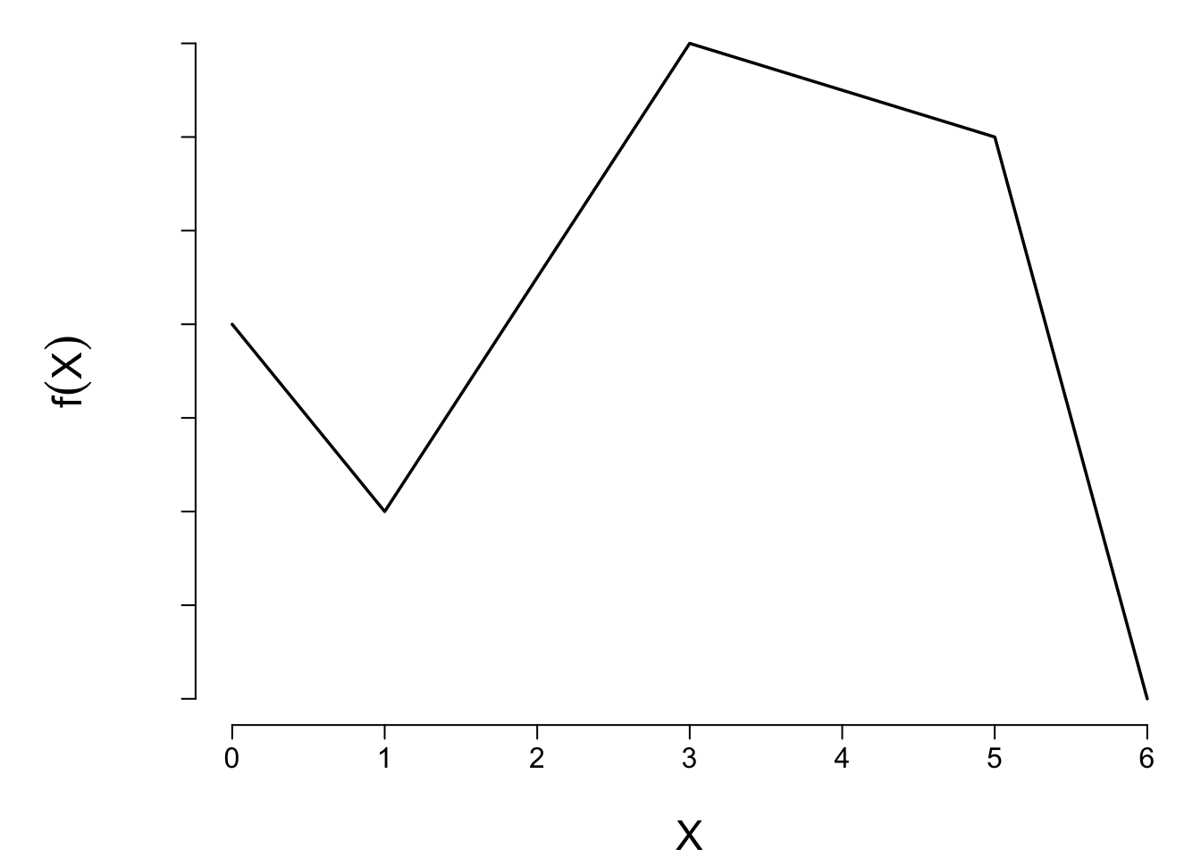
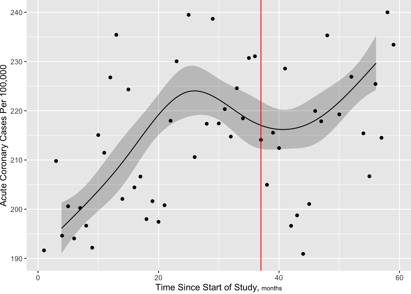
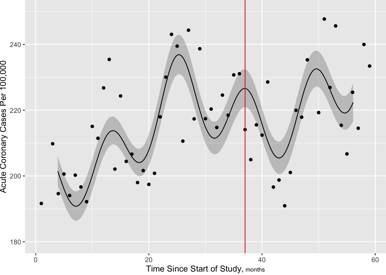
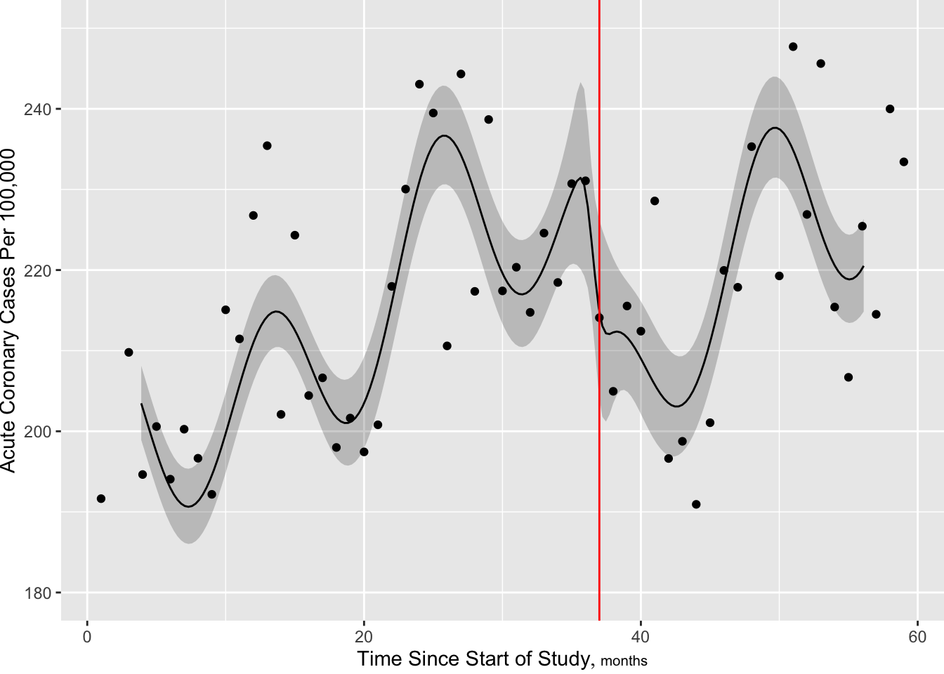
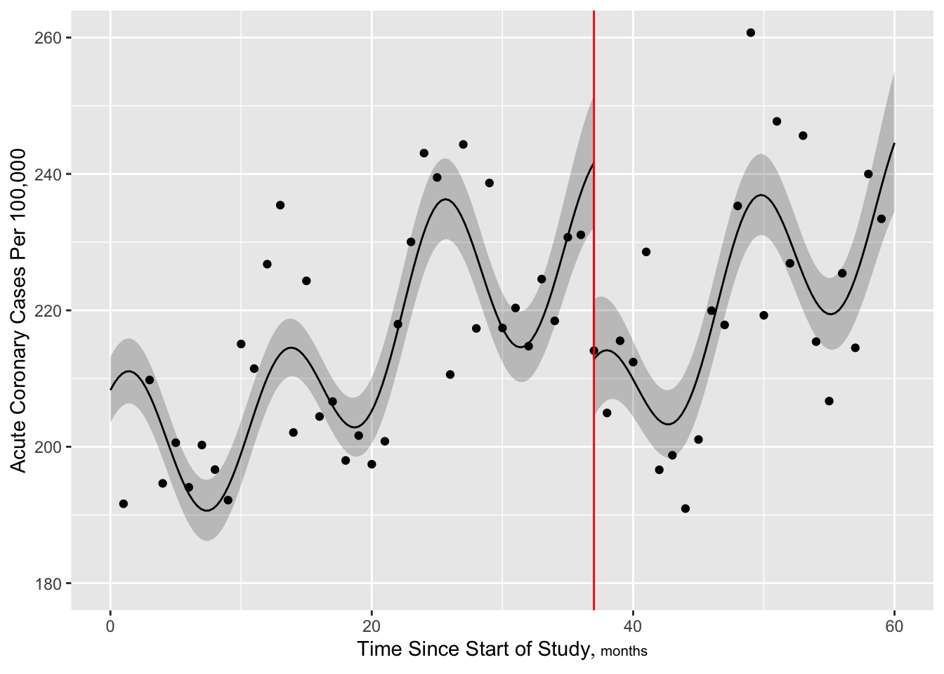
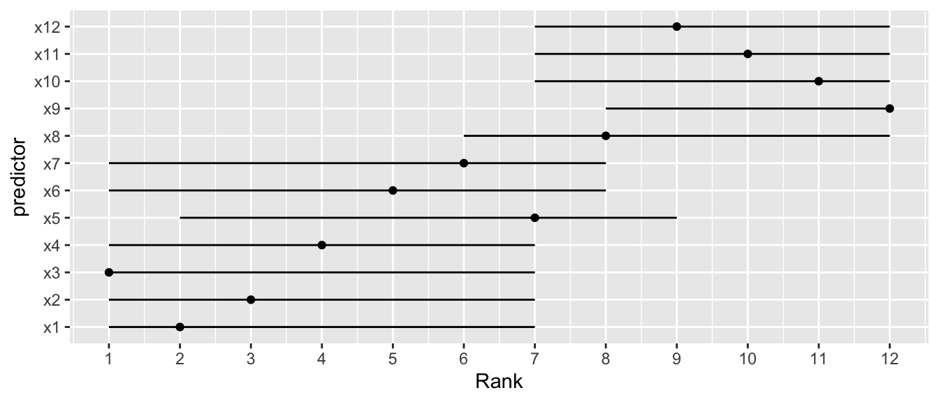
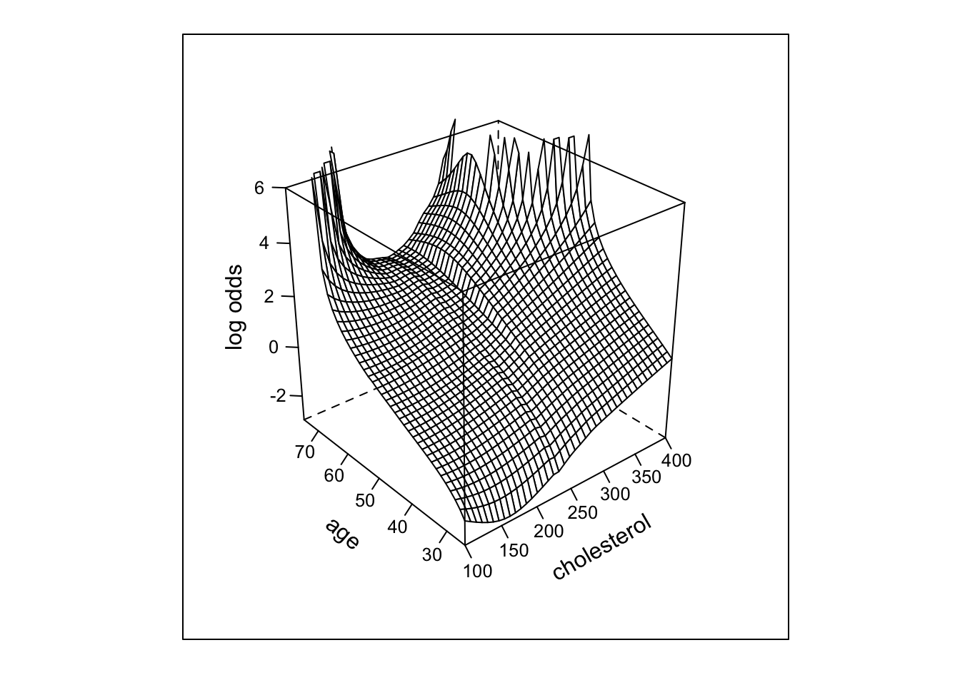
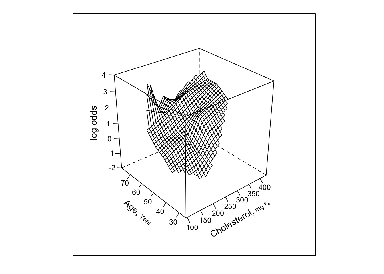
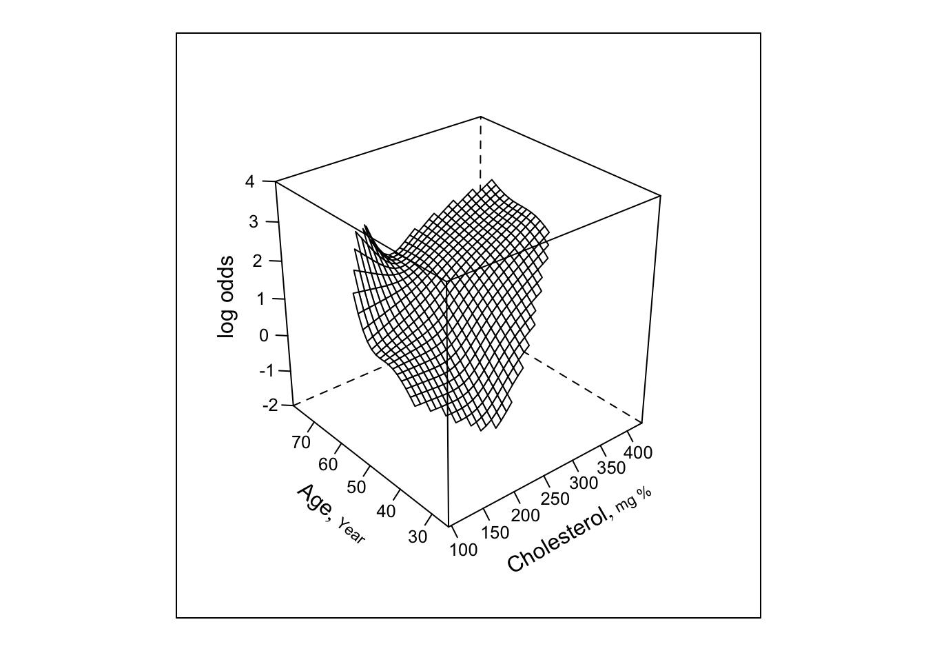
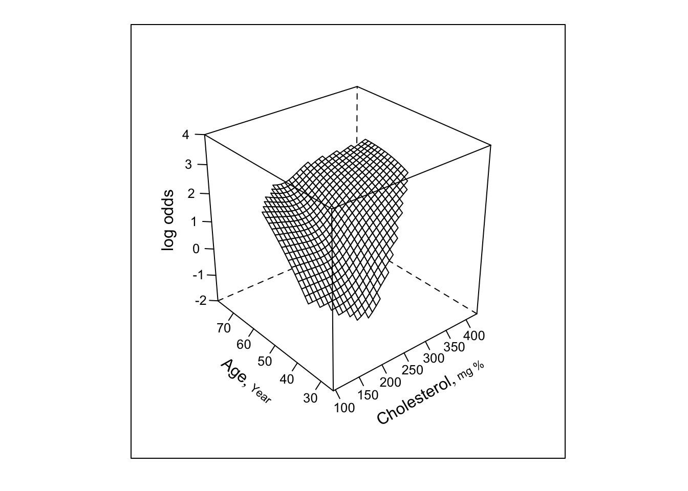
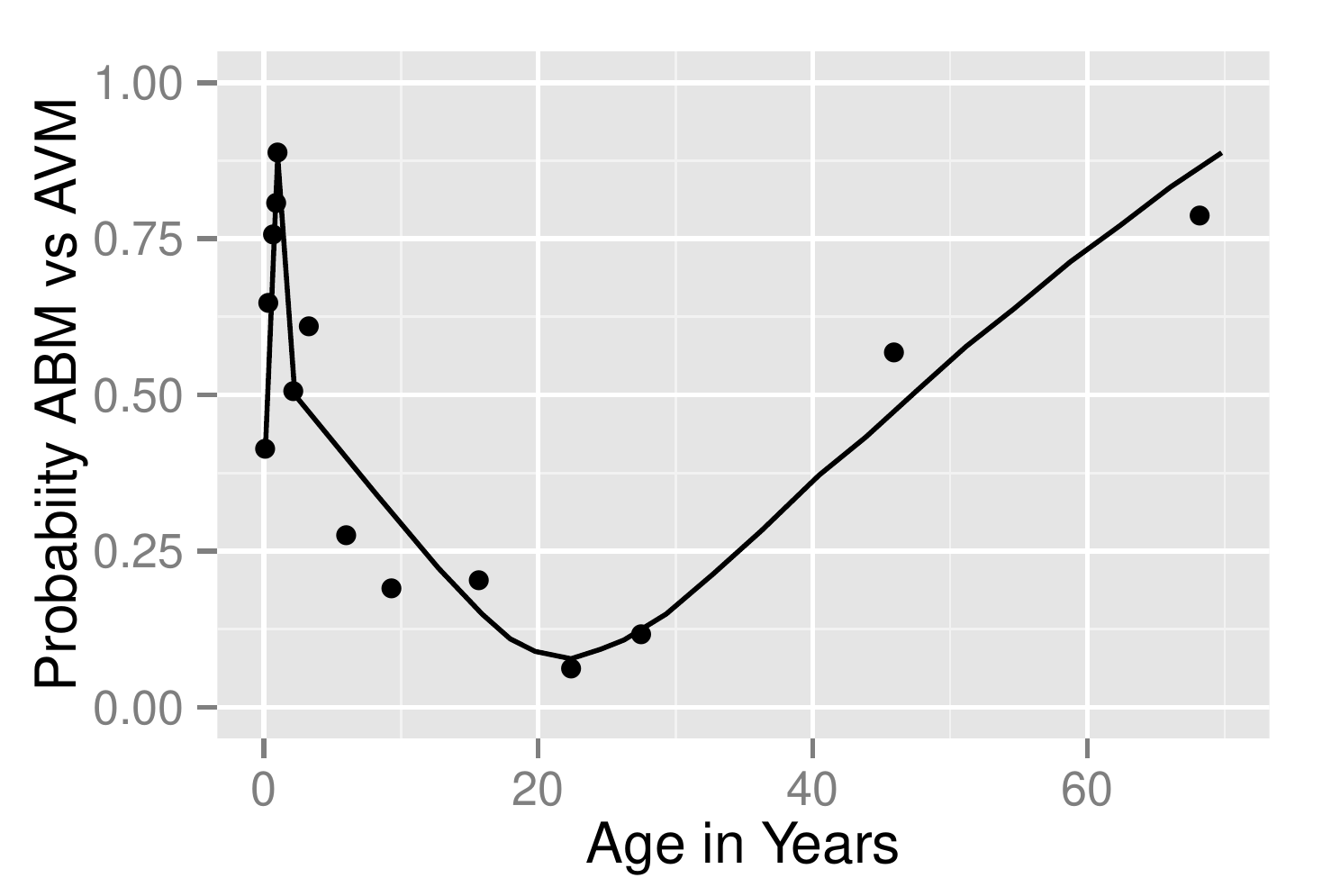
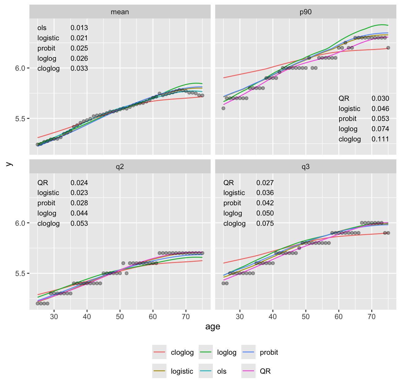
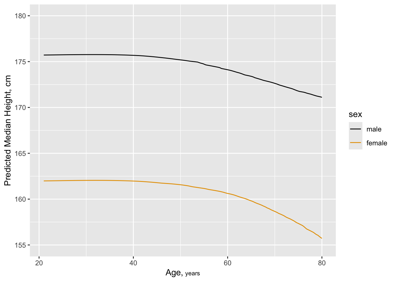
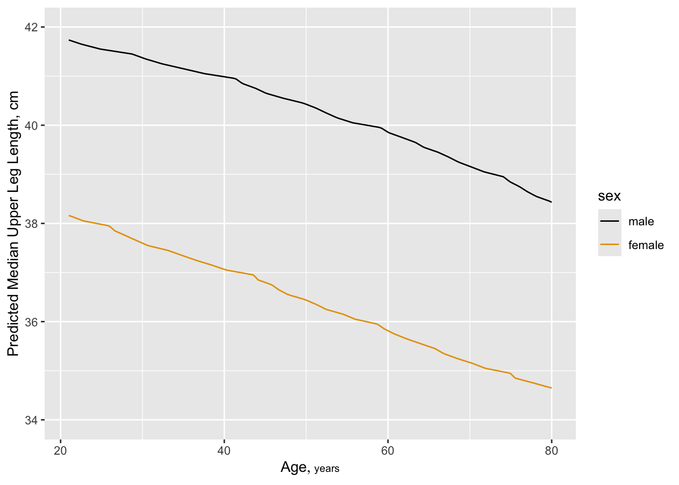
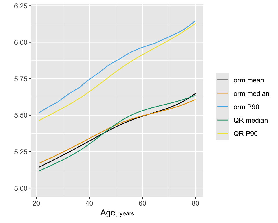
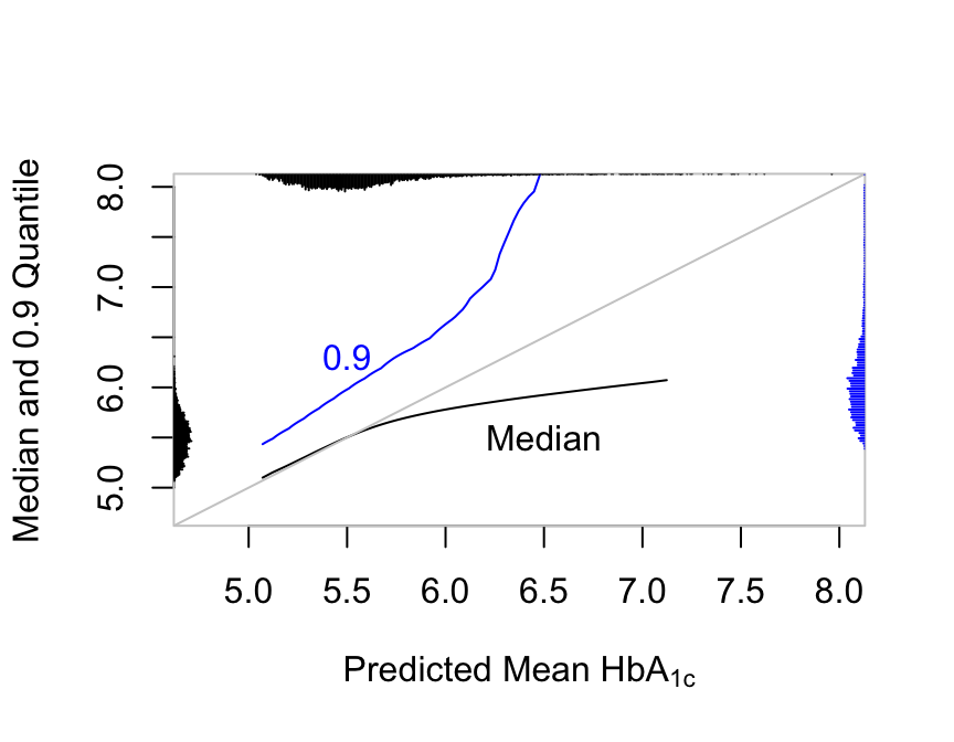
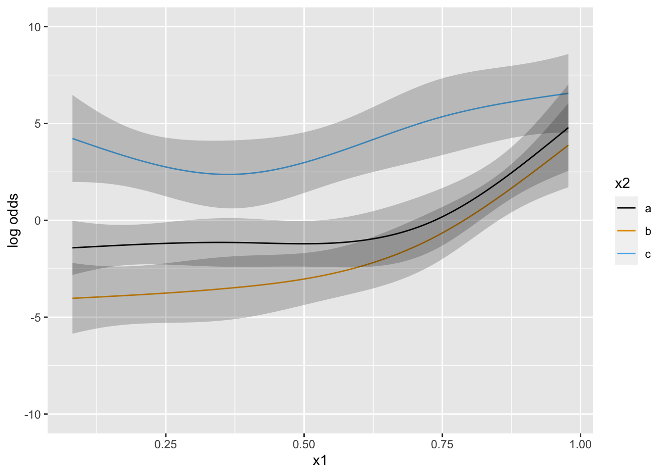
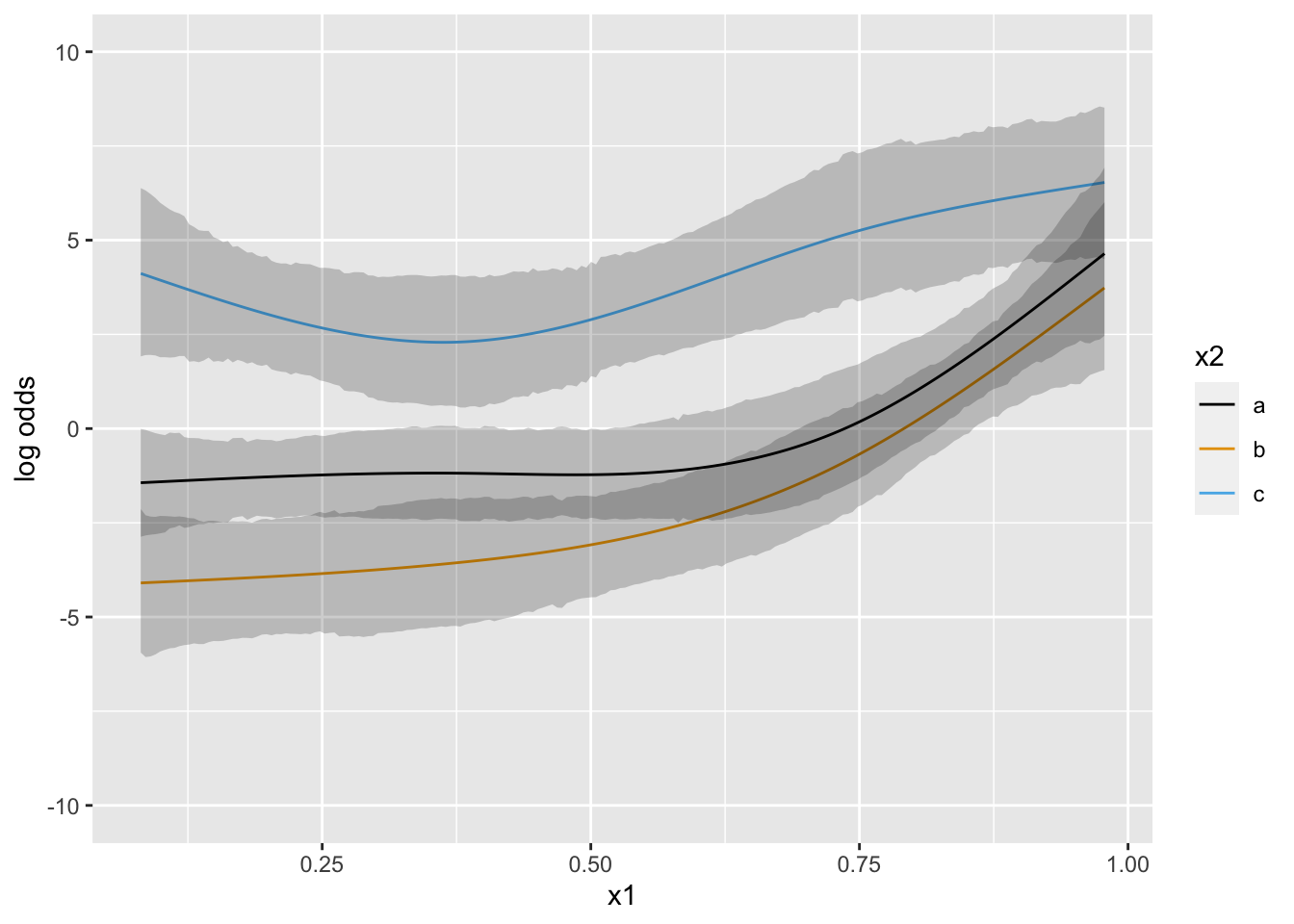
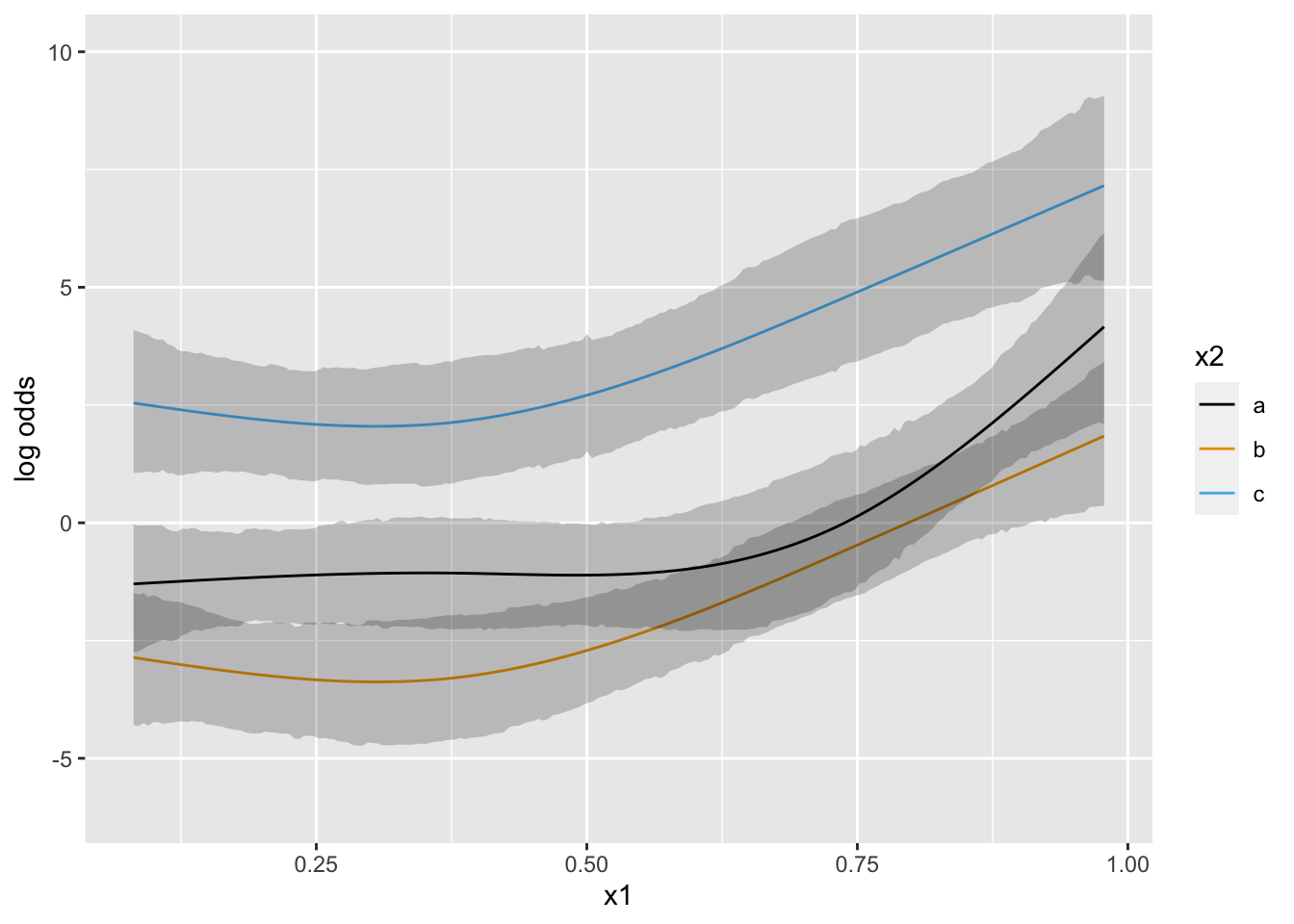
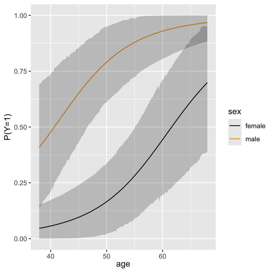
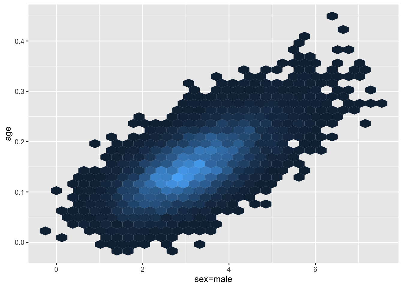
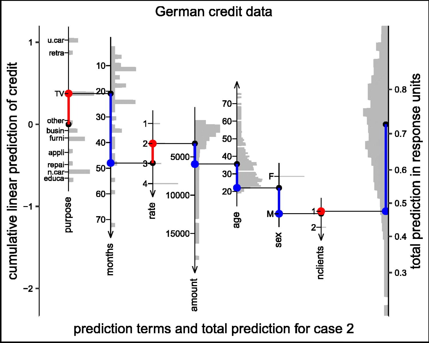Predictions plot from Rousseeuw (2026)

Contrasts

Forming contrasts through differences in predicted values is the most general and easy way to estimate effects of interest in a model. This is because

One needs only to specify two or more sets of predictor settings to contrast
Predictor coding, nonlinear terms, and interactions are automatically taken into account
Unspecified predictors can default to reference values such as medians for continuous predictors and modes for categorical ones. The values used for unspecified predictors only matter if they interact with predictors that are changing in the contrast.
Approximate methods are available for getting simultaneous confidence intervals over a whole sequence of contrasts (e.g., simultaneous confidence bands for an entire range of ages) when contrasts produce more than one estimate
The approach extends to any order of differences. E.g., interaction contrasts are formed with double differences.
Contrasts allow assessment of linearity over a given predictor range in a spline fit
Contrasts allow assessment of “partial interactions”, i.e., whether there is an interaction between one predictor and a subset of the levels of another predictor
The R predict function provides the $X$ (design matrix) that goes along with each requested prediction, and simple matrix algebra provides needed covariance matrices once differences in design matrices are formed

On the latter point, a single difference contrast such as one comparing 30 year old males with 40 year old males would generate two design matrices $X_{1}, X_{2}$, and the contrast $X_{1}\beta - X_{2}\beta = (X_{1} - X_{2})\beta$.

Consider a series of examples in which predicted values from a fitted model are symbolized by a function $f$ of the predictor settings, with continuous predictors $A$ and $B$ and a categorical predictor $C$ with levels $i, j, k$. Let the reference (detault) values of the predictors be $a$ (median of $A$), $b$ (median of $B$), and $c$ (modal (most frequent) category of $C$).

The term “average slope” used below will be the slope if the predictor has a linear effect, otherwise it is the average slope over the indicated interval. See here for more information.

Single Difference Contrasts

Average slope of $A$ over $A \in [1, 2]$: $f(2, b, c) - f(1, b, c)$
Difference between categories $j$ and $k$ in $C$: $f(a, b, j) - f(a, b, k)$
Effect of an entire range of predictor values against a single reference value: $f(1:10, b, c) - f(5, b, c)$ (a simultaneous confidence band would be useful here)

Double Difference Contrasts

Linearity in $A$ over $A \in [1, 3]$: $f(3, b, c) - f(2, b, c) - [f(2, b, c) - f(1, b, c)] = f(3, b, c) - 2f(2, b, c) + f(1, b, c)$
Interaction between $A$ and $C$ with respect to only two levels of $C$: $f(2, b, j) - f(1, b, j) - [f(2, b, k) - f(1, b, k)]$
Interaction between $A$ and $B$ when $A$ varies from 1 to 3 and $B$ varies from 5 to 6: $f(3, 5, c) - f(1, 5, c) - [f(3, 6, c) - f(1, 6, c)]$
Effect of $C=i$ vs. $C=j$ over a regular grid of values of $B$: $f(a, 5:15, i) - f(a, 5:15, j)$ (with possible simultaneous band; this is often a better way of getting hazard ratios in a Cox proportional hazards model, as the user has control of the reference value)

Triple Difference Contrasts

Third-order interactions
Assessment of nonlinearity in the $A\times B$ interaction (differences in double differences)

The R rms package contrast function (full name contrast.rms) provides predicted values, differences, and double difference contrasts. The latter is specified by providing four lists of predictor settings.

5.1.2 Indexes of Model Performance

Error Measures

Central tendency of prediction errors
- Mean absolute prediction error: mean $|Y - \hat{Y}|$
- Mean squared prediction error
  - Binary $Y$: Brier score (quadratic proper scoring rule)
- Logarithmic proper scoring rule (avg. log-likelihood)
Discrimination measures
- Pure discrimination: rank correlation of $(\hat{Y}, Y)$
  - Spearman $\rho$, Kendall $\tau$, Somers’ $D_{xy}$
  - $Y$ binary $\rightarrow$ $D_{xy} = 2\times (C - \frac{1}{2})$
    $C$ = concordance probability = area under receiver operating characteristic curve $\propto$ Wilcoxon-Mann-Whitney statistic
- Mostly discrimination: $R^{2}$
  - $R^{2}_{\mathrm{adj}}$—overfitting corrected if model pre-specified
- Brier score can be decomposed into discrimination and calibration components
- Discrimination measures based on variation in $\hat{Y}$
  - regression sum of squares
  - $g$–index
  - see here for related information
Calibration measures
- calibration–in–the–large: average $\hat{Y}$ vs. average $Y$
- high-resolution calibration curve (calibration–in–the–small). See ?fig-titanic-calibrate.
- calibration slope and intercept
- maximum absolute calibration error
- mean absolute calibration error
- 0.9 quantile of calibration error

See Van Calster et al. (2016) for a nice discussion of different levels of calibration stringency and their relationship to likelihood of errors in decision making.

$g$–Index

Based on Gini’s mean difference
- mean over all possible $i \neq j$ of $|Z_{i} - Z_{j}|$
- interpretable, robust, highly efficient measure of variation
$g =$ Gini’s mean difference of $X_{i}\hat{\beta} = \hat{Y}$
Example: $Y=$ systolic blood pressure; $g = 11$mmHg is typical difference in $\hat{Y}$
Independent of censoring etc.
For models in which anti-log of difference in $\hat{Y}$ represent meaningful ratios (odds ratios, hazard ratios, ratio of medians):
$g_{r} = \exp(g)$
For models in which $\hat{Y}$ can be turned into a probability estimate (e.g., logistic regression):
$g_{p} =$ Gini’s mean difference of $\hat{P}$
These $g$–indexes represent e.g. “typical” odds ratios, “typical” risk differences
Can define partial $g$

5.1.3 Relative Explained Variation

In OLS linear models $R^2$ is an excellent measure of explained variation in $Y$
Fraction of variance of $Y$ that is explained by $X$
SSR = $\sum_{i=1}^{n} (\hat{Y}_{i} - \bar{\hat{Y}})^2$ = regression sum of squares
- proportional to variance of $\hat{Y}$
SSE = $\sum_{i=1}^{n} (Y_{i} - \hat{Y}_{i})^2$ = error sum of squares = residual sum of squares
- proportional to error variance
SST = $\sum_{i=1}^{n} (Y_{i} - \bar{Y})^2$ = total sum of squares
- proportion to variance of $Y$
SST = SSR + SSE
$R^{2} =$ SSR/SST = 1 - SSE/SST
For each part of the model can compute its partial SSR = loss in SSR after refitting the model upon removing the part of the model being assessed
Partial $R^{2}$ = (partial SSR)/SST
Relative partial $R^{2} = \frac{\text{partial } R^{2}}{R^{2}} =$ partial SSR divided by full model SSR
Relative partial $R^{2}$ = portion of explainable (by $X$) variation in $Y$ that is explained by one or more terms in the model
Relative explained variation: REV
REVs do not need to sum to 1.0
- collinearities
- computing REVs for overlapping model terms
When a predictor interacts with another predictor, the predictor’s REV is taken from the combined predictive information in
- the predictor main effect (including any nonlinear terms)
- any interaction terms involving that effect

Extension to Other Models

For models fitted using maximum likelihood estimation, can compute the partial likelihood ratio $\chi^2$ statistic for each set and divide that by the total model LR $\chi^2$
See also Chapter 9 and the example below
This is an excellent measure but requires more computation and doesn’t extend to models not having a likelihood or to Bayesian modeling
Need a general purpose REV measure that works on virtually all models using all estimation techniques
Letting $\hat{Y} = X\hat{\beta}$ be the estimated linear predictor from the model
Use the same design matrix $X$ used to get $\hat{Y}$
Predict $\hat{Y}$ from $X$ using OLS
The $R^{2}$ from this model is 1.0
SSE = 0; ignore this and take variance-covariance matrix as $(X'X)^{-1}$ since SSR is used only on a relative basis
REV = $\frac{\text{partial SSR }}{\text{SSR}}$
Identical to relative $R^2$ if original model was OLS
Easily lends itself to uncertainty intervals
- frequentist: bootstrap the original model fit and save the repeated coefficient estimates (done by R rms package bootcov function); compute bootstrap confidence intervals for REVs; see Section 5.2 and example below
- Bayesian: compute REV for each posterior draw of $\beta$ and from the repeated REVs compute highest posterior density uncertainty intervals
Implemented in R rms package rexVar function

See Luchman (2014) for a nice review of log-likelihood-based relative importance measures.

Example

Ordinal regression model (proportional odds model for continuous Y)
Allow for quadratic effects for two predictors which are allowed to interact
Three other predictors that are irrelevant are modeled linearly
Bootstrap
Through uncertainty intervals for REVs show that when the sample size is inadequate for fitting an accurate reproducible model it’s also inadequate for measuring variable importance

Code

require(rms)
options(prType='html')
n <- 60
set.seed(3)
x1 <- rnorm(n)
x2 <- rnorm(n)
x3 <- rnorm(n)
x4 <- rnorm(n)
x5 <- rnorm(n)
y  <- round(x1 + x2 + rnorm(n), 2)
d  <- data.frame(x1, x2, x3, x4, y)
f  <- orm(y ~ pol(x1, 2) * pol(x2, 2) + x3 + x4 + x5,
          x=TRUE, y=TRUE)
a <- anova(f, test='LR')
a

1: Makes print methods output html for prettier printing
2: x=TRUE, y=TRUE are needed for later bootstrapping
3: Computes likelihood ratio $\chi^2$ test statistics for all partial effects in the model plus for the whole model

	χ²	d.f.	P
Likelihood Ratio Statistics for `y`
x1 (Factor+Higher Order Factors)	40.82	6	<0.0001
All Interactions	4.70	4	0.3190
Nonlinear (Factor+Higher Order Factors)	3.60	3	0.3082
x2 (Factor+Higher Order Factors)	29.90	6	<0.0001
All Interactions	4.70	4	0.3190
Nonlinear (Factor+Higher Order Factors)	3.80	3	0.2841
x3	0.09	1	0.7639
x4	1.14	1	0.2858
x5	0.17	1	0.6759
x1 × x2 (Factor+Higher Order Factors)	4.70	4	0.3190
Nonlinear	4.23	3	0.2373
Nonlinear Interaction : f(A,B) vs. AB	4.23	3	0.2373
f(A,B) vs. Af(B) + Bg(A)	1.68	1	0.1952
Nonlinear Interaction in x1 vs. Af(B)	3.55	2	0.1698
Nonlinear Interaction in x2 vs. Bg(A)	3.35	2	0.1872
TOTAL NONLINEAR	4.56	5	0.4718
TOTAL NONLINEAR + INTERACTION	5.80	6	0.4463
TOTAL	47.70	11	<0.0001

Code

plot(a, what='proportion chisq', sort='ascending')

1: Plots ratios of partial $\chi^2$ to total model LR $\chi^2$. ascending is really a misnomer.

Figure 5.1: Relative LR $\chi^2$ explained. Interaction effects are added to main effects.

Let’s use the bootstrap to get uncertainty intervals for relative explained variation. Note that for this small sample size, bootstrap parameter estimates are highly unstable and have standard errors that are about $4\times$ larger than the estimates from maximum likelihood estimation. We tell bootcov to only retain intercepts that target the median of y.

Code

# Have bootcov save only one intercept for each fit: the one corresponding to the
# median of y
g <- bootcov(f, B=300, ytarget=NA)
rx <- rexVar(g, data=d)
rx


Relative Explained Variation

          REV Lower Upper
x1      0.769 0.310 0.897
x2      0.508 0.322 0.898
x3      0.001 0.000 0.060
x4      0.017 0.000 0.192
x5      0.002 0.000 0.079
x1 * x2 0.056 0.027 0.544

Code

plot(rx)

Figure 5.2: Relative explained variation due to each predictor. Interaction effects are added to main effects. Intervals are 0.95 bootstrap percentile confidence intervals.

5.2 The Bootstrap

If know population model, use simulation or analytic derivations to study behavior of statistical estimator
Suppose $Y$ has a cumulative dist. fctn. $F(y) = \Pr\{Y \leq y\}$
We have sample of size $n$ from $F(y)$,
$Y_{1}, Y_{2}, \ldots, Y_{n}$
Steps:
1. Repeatedly simulate sample of size $n$ from $F$
2. Compute statistic of interest
3. Study behavior over $B$ repetitions
Example: 1000 samples, 1000 sample medians, compute their sample variance
$F$ unknown $\rightarrow$ estimate by empirical dist. fctn. \[ F_{n}(y) = \frac{1}{n}\sum_{i=1}^{n} [Y_{i} \leq y]. \]
Example: sample of size $n=30$ from a normal distribution with mean 100 and SD 10

Code

spar()
set.seed(6)
x <- rnorm(30, 100, 20)
xs <- seq(50, 150, length=150)
cdf <- pnorm(xs, 100, 20)
plot(xs, cdf, type='l', ylim=c(0,1),
     xlab=expression(x),
     ylab=expression(paste("Pr(", X <= x, ")")))
lines(ecdf(x), cex=.5)

Figure 5.3: Empirical and population cumulative distribution function

$F_{n}$ corresponds to density function placing probability $\frac{1}{n}$ at each observed data point ($\frac{k}{n}$ if point duplicated $k$ times)
Pretend that $F \equiv F_{n}$
Sampling from $F_{n} \equiv$ sampling with replacement from observed data $Y_{1},\ldots,Y_{n}$
Large $n$ $\rightarrow$ selects $1-e^{-1} \approx 0.632$ of original data points in each bootstrap sample at least once
Some observations not selected, others selected more than once
Efron’s bootstrap $\rightarrow$ general-purpose technique for estimating properties of estimators without assuming or knowing distribution of data $F$
Take $B$ samples of size $n$ with replacement, choose $B$ so that summary measure of individual statistics $\approx$ summary if $B=\infty$
Bootstrap based on distribution of observed differences between a resampled parameter estimate and the original estimate telling us about the distribution of unobservable differences between the original estimate and the unknown parameter

Example: Data $(1,5,6,7,8,9)$, obtain 0.80 confidence interval for population median, and estimate of population expected value of sample median (only to estimate the bias in the original estimate of the median).

Code

spar(ps=9, mfrow=c(1,2))
options(digits=3)
y <- c(2,5,6,7,8,9,10,11,12,13,14,19,20,21)
y <- c(1,5,6,7,8,9)
set.seed(17)
n   <- length(y)
n2  <- n/2
n21 <- n2+1
B   <- 400
M <- double(B)
plot(0, 0, xlim=c(0,B), ylim=c(3,9),
     xlab="Bootstrap Samples Used",
     ylab="Mean and 0.1, 0.9 Quantiles", type="n")
for(i in 1:B) {
  s <- sample(1:n, n, replace=T)
  x <- sort(y[s])
  m <- .5*(x[n2]+x[n21])
  M[i] <- m
  points(i, mean(M[1:i]), pch=46)
  if(i>=10) {
    q <- quantile(M[1:i], c(.1,.9))
    points(i, q[1], pch=46, col='blue')
    points(i, q[2], pch=46, col='blue')
  }
}
table(M)

M
  1   3 3.5   4 4.5   5 5.5   6 6.5   7 7.5   8 8.5   9 
  2   7   6   2   1  30  45  59  72  70  45  48   8   5

Code

hist(M, nclass=length(unique(M)), xlab="", main="")

Figure 5.4: Estimating properties of sample median using the bootstrap

First 20 samples:

Bootstrap Sample		Sample Median
1 5 5 7 8 9		6.0
1 1 5 7 9 9		6.0
6 7 7 8 9 9		7.5
1 1 5 6 8 9		5.5
1 6 7 7 8 8		7.0
1 5 6 8 8 9		7.0
1 6 8 8 9 9		8.0
5 5 6 7 8 9		6.5
1 5 6 7 7 8		6.5
1 5 6 8 9 9		7.0
1 5 7 7 8 9		7.0
1 5 6 6 7 8		6.0
1 6 6 7 8 9		6.5
5 6 7 7 8 9		7.0
1 5 6 8 8 8		7.0
1 1 6 6 7 8		6.0
5 5 5 8 8 9		6.5
5 6 6 6 7 7		6.0
1 5 7 9 9 9		8.0
1 1 5 5 5 7		5.0

Histogram tells us whether we can assume normality for the bootstrap medians or need to use quantiles of medians to construct C.L.
Need high $B$ for quantiles, low for variance (but see Booth & Sarkar (1998))
See Efron & Narasimhan (2020) for useful information about bootstrap confidence intervals and the latest R functions

5.3 Model Validation

5.3.1 Introduction

External validation (best: another country at another time); also validates sampling, measurements
Internal
- apparent (evaluate fit on same data used to create fit)
- data splitting
- cross-validation
- bootstrap: get overfitting-corrected accuracy index
Best way to make model fit data well is to discard much of the data (not recommended!)
Predictions on another dataset will be inaccurate
Need unbiased assessment of predictive accuracy

Working definition of external validation: Validation of a prediction tool on a sample that was not available at publication time.

Alternate: Validation of a prediction tool by an independent research team.

One suggested hierarchy of the quality of various validation methods is as follows, ordered from worst to best.

Attempting several validations (internal or external) and reporting only the one that “worked”
Reporting apparent performance on the training dataset (no validation)
Reporting predictive accuracy on an undersized independent test sample
Internal validation using data splitting where at least one of the training and test samples is not huge and the investigator is not aware of the arbitrariness of variable selection done on a single sample
Strong internal validation using 100 repeats of 10-fold cross-validation or several hundred bootstrap resamples, repeating all analysis steps involving $Y$ afresh at each re-sample and the arbitrariness of selected “important variables” is reported (if variable selection is used)
External validation on a large test sample, done by the original research team
Re-analysis by an independent research team using strong internal validation of the original dataset
External validation using new test data, done by an independent research team
External validation using new test data generated using different instruments/technology, done by an independent research team

Some points to consider:

Unless both sample sizes are huge, external validation can be low precision
External validation can be costly and slow and may result in disappointment that would have been revealed earlier with rigorous internal validation
External validation is sometimes gamed; researchers disappointed in the validation sometimes ask for a “do over”; resampling validation is harder to game as long as all analytical steps using $Y$ are repeated each time.
Instead of external validation to determine model applicability at a different time or place, and being disappointed if the model does not work in that setting, consider building a unified model containing time and place as predictors
When the model was fully pre-specified, external validation tests the model
But when the model was fitted using machine learning, feature screening, variable selection, or model selection, the model developed using training data is usually only an example of a model, and the test sample validation could be called an example validation
When resampling is used to repeat all modeling steps for each resample, rigorous internal validation tests the process used to develop the model and happens to also provide a high-precision estimate of the likely future performance of the “final” model developed using that process, properly penalizing for model uncertainty.
Resampling also reveals the volatility of the model selection process

$\rightarrow$ See BBR

Collins et al. (2016) estimate that a typical sample size needed for externally validating a time-to-event model is 200 events. Riley et al. (2024) has more in-depth guidance for sizing an external validation study.

5.3.2 Which Quantities Should Be Used in Validation?

OLS: $R^2$ is one good measure for quantifying drop-off in predictive ability
Example: $n=10, p=9$, apparent $R^{2}=1$ but $R^2$ will be close to zero on new subjects
Example: $n=20, p=10$, apparent $R^{2}=.9$, $R^2$ on new data 0.7, $R^{2}_{adj} = 0.79$
Adjusted $R^2$ solves much of the bias problem assuming $p$ in its formula is the largest number of parameters ever examined against $Y$
Few other adjusted indexes exist
Also need to validate models with phantom d.f.
Cross-validation or bootstrap can provide unbiased estimate of any index; bootstrap has higher precision
Two main types of quantities to validate
1. Calibration or reliability: ability to make unbiased estimates of response ($\hat{Y}$ vs. $Y$)
2. Discrimination: ability to separate responses
  OLS: $R^2$; $g$-index; binary logistic model: ROC area, equivalent to rank correlation between predicted probability of event and 0/1 event
Unbiased validation nearly always necessary, to detect overfitting

5.3.3 Data-Splitting

Split data into training and test sets
Interesting to compare index of accuracy in training and test
Freeze parameters from training
Make sure you allow $R^{2} = 1-SSE/SST$ for test sample to be $<0$
Don’t compute ordinary $R^2$ on $X\hat{\beta}$ vs. $Y$; this allows for linear recalibration $aX\hat{\beta} + b$ vs. $Y$
Test sample must be large enough to obtain very accurate assessment of accuracy
Training sample is what’s left
Example: overall sample $n=300$, training sample $n=200$, develop model, freeze $\hat{\beta}$, predict on test sample ($n=100$), $R^{2} = 1 - \frac{\sum(Y_{i}-X_{i}\hat{\beta})^{2}}{\sum(Y_{i}-\bar{Y})^{2}}$.
Disadvantages of data splitting:
1. Costly in $\downarrow n$ (Breiman, 1992; Roecker, 1991)
2. Requires decision to split at beginning of analysis
3. Requires larger sample held out than cross-validation
4. Results vary if split again
5. Does not validate the final model (from recombined data)
6. Not helpful in getting CL corrected for var. selection
7. Nice summary of disadvantages: Steyerberg (2018)

5.3.4 Improvements on Data-Splitting: Resampling

No sacrifice in sample size
Work when modeling process automated
Bootstrap excellent for studying arbitrariness of variable selection (Sauerbrei & Schumacher, 1992).
Cross-validation solves many problems of data splitting (Efron, 1983; Shao, 1993; van Houwelingen & le Cessie, 1990; Wu, 1986)
Example of $\times$-validation:
1. Split data at random into 10 tenths
2. Leave out $\frac{1}{10}$ of data at a time
3. Develop model on $\frac{9}{10}$, including any variable selection, pre-testing, etc.
4. Freeze coefficients, evaluate on $\frac{1}{10}$
5. Average $R^2$ over 10 reps
Drawbacks:
1. Choice of number of groups and repetitions
2. Doesn’t show full variability of var. selection
3. Does not validate full model
4. Lower precision than bootstrap
5. Need to do 50 repeats of 10-fold cross-validation to ensure adequate precision
Randomization method
1. Randomly permute $Y$
2. Optimism = performance of fitted model compared to what expect by chance

5.3.5 Validation Using the Bootstrap

Estimate optimism of final whole sample fit without holding out data
From original $X$ and $Y$ select sample of size $n$ with replacement
Derive model from bootstrap sample
Apply to original sample
Simple bootstrap uses average of indexes computed on original sample
Estimated optimism = difference in indexes
Repeat about $B=100$ times, get average expected optimism
Subtract average optimism from apparent index in final model
Example: $n=1000$, have developed a final model that is hopefully ready to publish. Call estimates from this final model $\hat{\beta}$.
- final model has apparent $R^2$ ($R^{2}_{app}$) =0.4
- how inflated is $R^{2}_{app}$?
- get resamples of size 1000 with replacement from original 1000
- for each resample compute $R^{2}_{boot}$ = apparent $R^2$ in bootstrap sample
- freeze these coefficients (call them $\hat{\beta}_{boot}$), apply to original (whole) sample $(X_{orig}, Y_{orig})$ to get $R^{2}_{orig} = R^{2}(X_{orig}\hat{\beta}_{boot}, Y_{orig})$
- optimism = $R^{2}_{boot} - R^{2}_{orig}$
- average over $B=100$ optimisms to get $\overline{optimism}$
- $R^{2}_{overfitting~corrected} = R^{2}_{app} - \overline{optimism}$

Example: Chapter 8
Is estimating unconditional (not conditional on $X$) distribution of $R^2$, etc. (Faraway, 1992, p. 217)
Conditional estimates would require assuming the model one is trying to validate
Efron’s “$.632$” method may perform better (reduce bias further) for small $n$ (Efron, 1983), (Efron & Tibshirani, 1993, p. 253), Efron & Tibshirani (1997)

Bootstrap useful for assessing calibration in addition to discrimination:

Fit $C(Y|X) = X\beta$ on bootstrap sample
Re-fit $C(Y|X) = \gamma_{0} + \gamma_{1}X\hat{\beta}$ on same data
$\hat{\gamma}_{0}=0, \hat{\gamma}_{1}=1$
Test data (original dataset): re-estimate $\gamma_{0}, \gamma_{1}$
$\hat{\gamma}_{1}<1$ if overfit, $\hat{\gamma}_{0} > 0$ to compensate
$\hat{\gamma}_{1}$ quantifies overfitting and useful for improving calibration (Spiegelhalter, 1986)
Use Efron’s method to estimate optimism in $(0,1)$, estimate $(\gamma_{0}, \gamma_{1})$ by subtracting optimism from $(0,1)$
See also Copas (1987) and van Houwelingen & le Cessie (1990), p. 1318

See Freedman et al. (1988) for warnings about the bootstrap, and Efron (1983) for variations on the bootstrap to reduce bias.

Use bootstrap to choose between full and reduced models:

Bootstrap estimate of accuracy for full model
Repeat, using chosen stopping rule for each re-sample
Full fit usually outperforms reduced model(Spiegelhalter, 1986)
Stepwise modeling often reduces optimism but this is not offset by loss of information from deleting marginal var.

Method	Apparent Rank Correlation of Predicted vs. Observed	Over-optimism	Bias-Corrected Correlation
Full Model	0.50	0.06	0.44
Stepwise Model	0.47	0.05	0.42

In this example, stepwise modeling lost a possible $0.50 - 0.47 = 0.03$ predictive discrimination. The full model fit will especially be an improvement when

The stepwise selection deleted several variables which were almost significant.
These marginal variables have some real predictive value, even if it’s slight.
There is no small set of extremely dominant variables that would be easily found by stepwise selection.

Other issues:

See van Houwelingen & le Cessie (1990) for many interesting ideas
Faraway (1992) shows how bootstrap is used to penalize for choosing transformations for $Y$, outlier and influence checking, variable selection, etc. simultaneously
Brownstone (1988), p. 74 feels that “theoretical statisticians have been unable to analyze the sampling properties of (usual multi-step modeling strategies) under realistic conditions” and concludes that the modeling strategy must be completely specified and then bootstrapped to get consistent estimates of variances and other sampling properties
See Blettner & Sauerbrei (1993) and Chatfield (1995) for more interesting examples of problems resulting from data-driven analyses.

Confidence Intervals for Overfitting-Corrected Model Performance Measures

Uncertainty comes from estimating
- apparent performance
- bias in apparent performance (overfitting)
Noma et al. (2021) studied an accurate double-bootstrap-loop approach accounting for both sources of uncertainty
They also studied an approximate method where bootstrap percentile confidence intervals in the apparent accuracy were merely shifted by the estimated about of bias
The approximate approach requires no additional computations whereas the full double-loop approach is very slow
The authors found that the approximate solution works reasonably well if
- the sample size is not small
- the amount of overfitting is not huge

Examples with a small sample size and much overfitting showed the Noma et al fast shifted coinfidence intervals to not have adequate coverage due to accounting for only one source of uncertainty. An alternative called ABCLOC (asymmetric bootstrap confidence limits for overfitting-corrected model performance metrics) that was derived empirically for such situations has the best coverage to date from among fast methods not requiring an outer bootstrap loop. ABCLOC was derived and studied here. Briefly, it considers variation over bootstrap resamples in the quantity $\theta_{b} + 1.25 \theta_{w}$ where $\theta_{b}$ is a model performance measure for a model fitted and evaluated on a bootstrap sample, and $\theta_{w}$ is the measure from the model fitted on the bootstrap sample and evaluated on the original whole sample. Dual standard deviations of this quantity are computed to handle asymmetry of distributions. Confidence limits are the overfitting-corrected performance estimates $- a$ and the estimates $+ b$ where $a$ is the SD of the upper half of the distribution and $b$ is the SD for the lower half. A standard normal critical value is multipled by each SD.

ABCLOC limits are implemented in rms in version 8.1-0 for validate and calibrate functions.

5.3.7 Validation of Data Reduction

A frequently asked question is whether or not unsupervised learning (data reduction) needs to be repeated inside an internal validation loop. See this for some excellent discussion. Here are are few thoughts.

To be safe, include fresh data reduction inside each loop
If you want to take a slight risk you can do the data reduction once on the whole dataset, because of the following
Principal components (especially minor components), variable and observation clustering, and redundancy analysis can be very unstable
They way in which they are unstable is uninformed by $Y$, so this instability can work either for or against you
Typically we are allowed to use procedures that don’t always work in our favor
Contrast this with stepwise variable selection, which always attempts to work in our favor by maximizing $R^2$

5.3.8 Validation of Bayesian Models

Ideas about model validation can be much different in a Bayesian modeling context. If a prior distribution on a regression coefficient is somewhat flat, that implies that very large values of the parameter are likely. So overfitting cannot officially occur in that setting. Valuable discussions about Bayesian validation issues can be found here and here.

On the other hand, overfitting can damage out-of-sample predictive accuracy, and there are Bayesian Markov chain Monte Carlo shortcuts that provide leave-out-one cross-validation statistics on the gold standard log-likelihood metric. This is elegantly covered in this Richard McElreath video.

5.4 Bootstrapping Ranks of Predictors

Order of importance of predictors not pre-specified
Researcher interested in determining “winners” and “losers”
Bootstrap useful in documenting the difficulty of this task
Get confidence limits of the rank of each predictor in the scale of partial $\chi^2$ - d.f.
Example using OLS

Code

# Use the plot method for anova, with pl=FALSE to suppress actual
# plotting of chi-square - d.f. for each bootstrap repetition.
# Rank the negative of the adjusted chi-squares so that a rank of
# 1 is assigned to the highest.  It is important to tell
# plot.anova.rms not to sort the results, or every bootstrap
# replication would have ranks of 1,2,3,... for the stats.
require(rms)
n <- 300
set.seed(1)
d <- data.frame(x1=runif(n), x2=runif(n), x3=runif(n), x4=runif(n),
                x5=runif(n), x6=runif(n), x7=runif(n), x8=runif(n),
             x9=runif(n), x10=runif(n), x11=runif(n), x12=runif(n))
d$y <- with(d, 1*x1 + 2*x2 +  3*x3  +  4*x4  + 5*x5 + 6*x6 + 7*x7 +
               8*x8 + 9*x9 + 10*x10 + 11*x11 + 12*x12 + 9*rnorm(n))

f <- ols(y ~ x1+x2+x3+x4+x5+x6+x7+x8+x9+x10+x11+x12, data=d)
B <- 1000
ranks <- matrix(NA, nrow=B, ncol=12)
rankvars <- function(fit)
  rank(plot(anova(fit), sort='none', pl=FALSE))
Rank <- rankvars(f)
for(i in 1:B) {    # 6s
  j <- sample(1:n, n, TRUE)
  bootfit <- update(f, data=d, subset=j)
  ranks[i,] <- rankvars(bootfit)
  }
lim <- t(apply(ranks, 2, quantile, probs=c(.025,.975)))
predictor <- factor(names(Rank), names(Rank))
w <- data.frame(predictor, Rank, lower=lim[,1], upper=lim[,2])
require(ggplot2)
ggplot(w, aes(x=predictor, y=Rank)) + geom_point() + coord_flip() +
  scale_y_continuous(breaks=1:12) +
  geom_errorbar(aes(ymin=lim[,1], ymax=lim[,2]), width=0)

Figure 5.5: Bootstrap percentile 0.95 confidence limits for ranks of predictors in an OLS model. Ranking is on the basis of partial $\chi^2$ minus d.f. Point estimates are original ranks

See this and this for a higher-dimension example. See this for a more in-depth discussion of ranking variable importance.

5.6 How Do We Break Bad Habits?

Insist on validation of predictive models and discoveries
Show collaborators that split-sample validation is not appropriate unless the number of subjects is huge
- Split more than once and see volatile results
- Calculate a confidence interval for the predictive accuracy in the test dataset and show that it is very wide
Run simulation study with no real associations and show that associations are easy to find
Analyze the collaborator’s data after randomly permuting the $Y$ vector and show some positive findings
Show that alternative explanations are easy to posit
- Importance of a risk factor may disappear if 5 “unimportant” risk factors are added back to the model
- Omitted main effects can explain apparent interactions
- Uniqueness analysis: attempt to predict the predicted values from a model derived by data torture from all of the features not used in the model

10.1 Model

\[ \Pr(Y=1|X) = [1+\exp(-X\beta)]^{-1} \]

\[ P = [1+\exp(-x)]^{-1} = \text{expit}(x) \]

$O = \frac{P}{1-P}$
$P = \frac{O}{1+O}$
$X\beta = \log\frac{P}{1-P} = \text{logit}(P)$
$e^{X\beta} = O$

10.1.1 Model Assumptions and Interpretation of Parameters

\[\begin{array}{ccc} \text{logit}(Y=1|X) &=& \text{logit}(P) = \log\frac{P}{1-P} \nonumber \\ &=& X\beta , \end{array}\]

Increase $X_{j}$ by $d$ $\rightarrow$ increase odds $Y=1$ by $\exp(\beta_{j}d)$, increase log odds by $\beta_{j}d$.
If there is only one predictor $X$ and that predictor is binary, the model can be written

\[\begin{array}{ccc} \text{logit}(Y=1|X=0) &=& \beta_{0} \nonumber \\ \text{logit}(Y=1|X=1) &=& \beta_{0}+\beta_{1} . \end{array}\]

One continuous predictor: \[ \text{logit}(Y=1|X) = \beta_{0}+\beta_{1} X, \]
Two treatments (indicated by $X_{1}=0$ or $1$) and one continuous covariable ($X_{2}$). \[ \text{logit}(Y=1|X) = \beta_{0}+\beta_{1}X_{1}+\beta_{2}X_{2} , \]

\[\begin{array}{ccc} \text{logit}(Y=1|X_{1}=0, X_{2}) &=& \beta_{0}+\beta_{2}X_{2} \nonumber \\ \text{logit}(Y=1|X_{1}=1, X_{2}) &=& \beta_{0}+\beta_{1}+\beta_{2}X_{2} . \end{array}\]

10.1.2 Odds Ratio, Risk Ratio, and Risk Difference

Odds ratio capable of being constant
Ex: risk factor doubles odds of disease

Without Risk Factor		With Risk Factor
Probability	Odds	Odds	Probability
0.20	0.25	0.5	0.333
0.50	1.00	2.0	0.667
0.80	4.00	8.0	0.889
0.90	9.00	18.0	0.947
0.98	49.00	98.0	0.990

Code

spar(bty='l')
plot(0, 0, type="n", xlab="Risk for Subject Without Risk Factor",
     ylab="Increase in Risk",
     xlim=c(0,1), ylim=c(0,.6))
i <- 0
or <- c(1.1,1.25,1.5,1.75,2,3,4,5,10)
for(h in or) {
  i <- i + 1
  p <- seq(.0001, .9999, length=200)
  logit <- log(p/(1 - p))  # same as qlogis(p)
  logit <- logit + log(h)  # modify by odds ratio
  p2 <- 1/(1 + exp(-logit))# same as plogis(logit)
  d <- p2 - p
  lines(p, d, lty=i)
  maxd <- max(d)
  smax <- p[d==maxd]
  text(smax, maxd + .02, format(h), cex=.6)
}

Figure 10.2: Absolute benefit as a function of risk of the event in a control subject and the relative effect (odds ratio) of the risk factor. The odds ratios are given for each curve.

Let $X_{1}$ be a binary risk factor and let
$A=\{X_{2},\ldots,X_{p}\}$ be the other factors. Then the estimate of $\Pr(Y=1|X_{1}=1, A) -$ $\Pr(Y=1|X_{1}=0, A)$ is

\[\begin{array}{c} \frac{1}{1+\exp-[\hat{\beta_{0}}+\hat{\beta_{1}}+\hat{\beta_{2}}X_{2}+\ldots+\hat{\beta_{p}}X_{p}]} \nonumber \\ - \frac{1}{1+\exp-[\hat{\beta_{0}}+\hat{\beta_{2}}X_{2}+\ldots +\hat{\beta_{p}}X_{p}]} \\ = \frac{1}{1+(\frac{1-\hat{R}}{\hat{R}}) \exp(-\hat{\beta}_{1})} - \hat{R}, \nonumber \end{array}\]

where $R=\Pr(Y=1|X_{1}=0, A)$.

Risk ratio is $\frac{1+e^{-X_{2}\beta}}{1+e^{-X_{1}\beta}}$
Does not simplify like odds ratio, which is $\frac{e^{X_{1}\beta}}{e^{X_{2}\beta}} = e^{(X_{1}-X_{2})\beta}$

10.1.3 Detailed Example

Age: Females	37	39	39	42	47	48	48	52	53	55	56	57	58	58	60	64	65	68	68	70
Response:	0	0	0	0	0	0	1	0	0	0	0	0	0	1	0	0	1	1	1	1
Age: Males	34	38	40	40	41	43	43	43	44	46	47	48	48	50	50	52	55	60	61	61
Response:	1	1	0	0	0	1	1	1	0	0	1	1	1	0	1	1	1	1	1	1

Code

require(rms)
options(prType='html')     # output format for certain rms functions
getHdata(sex.age.response)
d <- as.data.table(sex.age.response)  # so can do easy aggregation
dd <- datadist(d); options(datadist='dd')
f <- lrm(response ~ sex + age, data=d)
fasr <- f   # Save for later
p <- Predict(f, age=seq(34, 70, length=200), sex, fun=plogis)
# Function to bin a variable and represent bin by mean x within bin
mb <- function(x, ...) as.numeric(as.character(cut2(x, ..., levels.mean=TRUE)))
d[, ageg := mb(age, cuts=c(45, 55))]
props <- d[, .(prop = mean(response)), by=.(ageg, sex)]
ggplot(p, ylab='Pr(response)') +
  geom_point(data=d, aes(x=age, y=response, color=sex)) +
  geom_point(data=props, aes(x=ageg, y=prop, color=sex, shape=I(2)))

Figure 10.3: Data, subgroup proportions (triangles), and fitted logistic model, with 0.95 pointwise confidence bands

Code

ltx <- function(fit) {
  w <- latex(fit, inline=TRUE, columns=54,
             after='', digits=3,
             before='$$X\\hat{\\beta}=$$')
    rendHTML(w, html=FALSE)
  }
ltx(f)

\[X\hat{\beta}=\]

\[\begin{array}{l} -9.84\\ +3.49[\mathrm{male}] +0.158\:\mathrm{age} \end{array}\]


                 sex        response
                 Frequency
                 Row Pct      0        1    Total     Odds/Log

                 F           14        6       20    6/14=.429
                          70.00    30.00                 -.847

                 M            6       14       20    14/6=2.33
                          30.00    70.00                  .847

                 Total       20       20       40

                M:F odds ratio = (14/6)/(6/14) = 5.44, log=1.695

sex $\times$ response
Statistic	DF	Value	Prob
Wald $\chi^2$	1	6.400	0.011
Likelihood Ratio $\chi^2$	1	6.583	0.010

Parameter	Estimate	Std Err	Wald $\chi^{2}$	P
$\beta_{0}$	-0.847	0.488	3.015
$\beta_{1}$	1.695	0.690	6.030	0.014

Log likelihood ($\beta_{1}=0$)	-27.727
Log likelihood (max)	-24.435
LR $\chi^{2} (H_{0}:\beta_{1}=0)$ -2(-27.727- -24.435) = 6.584

Next, consider the relationship between age and response, ignoring sex.

                 age        response
                 Frequency
                 Row Pct      0        1    Total     Odds/Log

                 <45          8        5       13     5/8=.625
                           61.5     38.4                  -.47

                 45-54        6        6       12        6/6=1
                           50.0     50.0                     0

                 55+          6        9       15      9/6=1.5
                           40.0     60.0                  .405

                 Total       20       20       40

                55+ : <45 odds ratio = (9/6)/(5/8) = 2.4, log=.875

Parameter	Estimate	Std Err	Wald $\chi^{2}$	P
$\beta_{0}$	-2.734	1.838	2.213
$\beta_{1}$	0.054	0.036	2.276	0.131

The estimate of $\beta_{1}$ is in rough agreement with that obtained from the frequency table. The 55+:<45 log odds ratio is .875, and since the respective mean ages in the 55+ and <45 age groups are 61.1 and 40.2, an estimate of the log odds ratio increase per year is .875/(61.1 - 40.2)=.875/20.9=.042.

The likelihood ratio test for $H_{0}$: no association between age and response is obtained as follows:

Log likelihood ($\beta_{1}=0$)	-27.727
Log likelihood (max)	-26.511
LR $\chi^{2} (H_{0}:\beta_{1}=0)$	-2(-27.727- -26.511) = 2.432

(Compare 2.432 with the Wald statistic 2.28.)

Next we consider the simultaneous association of age and sex with response.


                                 sex=F

                 age        response
                 Frequency
                 Row Pct      0        1    Total

                 <45          4        0        4
                          100.0      0.0

                 45-54        4        1        5
                           80.0     20.0

                 55+          6        5       11
                           54.6     45.4

                 Total       14        6       20


                                 sex=M

                 age        response
                 Frequency
                 Row Pct      0        1    Total

                 <45          4        5        9
                           44.4     55.6

                 45-54        2        5        7
                           28.6     71.4

                 55+          0        4        4
                            0.0    100.0

                 Total        6       14       20

A logistic model for relating sex and age simultaneously to response is given below.

Parameter	Estimate	Std Err	Wald $\chi^{2}$	P
$\beta_{0}$	-9.843	3.676	7.171
$\beta_{1}$ (sex)	3.490	1.199	8.469	0.004
$\beta_{2}$ (age)	0.158	0.062	6.576	0.010

Likelihood ratio tests are obtained from the information below.

Log likelihood ($\beta_{1}=0,\beta_{2}=0$)	-27.727
Log likelihood (max)	-19.458
Log likelihood ($\beta_{1}=0$)	-26.511
Log likelihood ($\beta_{2}=0$)	-24.435
LR $\chi^{2}$ ($H_{0}:\beta_{1}=\beta_{2}=0$)	-2(-27.727- -19.458)= 16.538
LR $\chi^{2}$ ($H_{0}:\beta_{1}=0$) sex$\|$age	-2(-26.511- -19.458) = 14.106
LR $\chi^{2}$ ($H_{0}:\beta_{2}=0$) age$\|$sex	-2(-24.435- -19.458) = 9.954

The 14.1 should be compared with the Wald statistic of 8.47, and 9.954 should be compared with 6.58. Likelihood ratio tests may be obtained automatically starting in rms version 6.7-0, as follows.

Code

f <- update(f, x=TRUE, y=TRUE)   # LR tests require raw data in fits
anova(f, test='LR')

	χ²	d.f.	P
Likelihood Ratio Statistics for `response`
sex	14.11	1	0.0002
age	9.95	1	0.0016
TOTAL	16.54	2	0.0003

The fitted logistic model is plotted separately for females and males in Figure 10.3 .

The fitted model is

\[\Pr(\text{Response=1}|\text{sex,age}) = \text{expit}(-9.84+3.49\times \text{sex} +.158\times \text{age})\]

where as before sex=0 for females, 1 for males. For example, for a 40 year old female, the predicted logit is $-9.84+.158(40) = -3.52$. The predicted probability of a response is $\text{expit}(3.52)= .029$. For a 40 year old male, the predicted logit is $-9.84 + 3.49+.158(40) = -.03$, with a probability of .492.

10.1.4 Design Formulations

Can do ANOVA using $k-1$ dummies for a $k$-level predictor
Can get same $\chi^2$ statistics as from a contingency table
Can go farther: covariable adjustment
Simultaneous comparison of multiple variables between two groups: Turn problem backwards to predict group from all the dependent variables
This is more robust than a parametric multivariate test
Propensity scores for adjusting for nonrandom treatment selection: Predict treatment from all baseline variables
Adjusting for the predicted probability of getting a treatment adjusts adequately for confounding from all of the variables
In a randomized study, using logistic model to adjust for covariables, even with perfect balance, will improve the treatment effect estimate

10.2 Estimation

10.2.1 Maximum Likelihood Estimates

Like binomial case but $P$s vary; $\hat{\beta}$ computed by trial and error using an iterative maximization technique

10.2.2 Estimation of Odds Ratios and Probabilities

\[\hat{P}_{i} = \text{expit}(X_{i}\hat{\beta})\]

\[\text{expit}(X_{i}\hat{\beta}\pm zs)\]

10.2.3 Minimum Sample Size Requirement

See this and this for detailed examples of power-based sample size calculations for the proportional odds model

Categorical Predictor Case

Simplest case: no covariates, only an intercept
Consider margin of error of 0.1 in estimating $\theta = \Pr(Y=1)$ with 0.95 confidence
Worst case: $\theta = \frac{1}{2}$
Requires $n=96$ observations¹
Single binary predictor with prevalence $\frac{1}{2}$: need $n=96$ for each value of $X$
For margin of error of $\pm 0.05, n=384$ is required (if true probabilities near 0.5 are possible); $n=246$ required if true probabilities are only known not to be in $[0.2, 0.8]$.

¹ The general formula for the sample size required to achieve a margin of error of $\delta$ in estimating a true probability of $\theta$ at the 0.95 confidence level is $n = (\frac{1.96}{\delta})^{2} \times \theta(1 - \theta)$. Set $\theta = \frac{1}{2}$ for the worst case.

Single Continuous Predictor

Predictor $X$ has a normal distribution with mean zero and standard deviation $\sigma$, with true $P = \text{expit}(X)$ so that the expected number of events is $\frac{n}{2}$. Compute mean and 0.9 quantile of $\max_{X \in [-1.5,1.5]} |P - \hat{P}|$ over 1000 simulations for varying $n$ and $\sigma$²

² An average absolute error of 0.05 corresponds roughly to a 0.95 confidence interval margin of error of 0.1.

See this for more about R coding for simulations of this type.

Code

require(rms)
require(ggplot2)

g <- function() {
set.seed(12)
sigmas  <- c(.5, .75, 1, 1.25, 1.5, 1.75, 2, 2.5, 3, 4)
ns      <- seq(25, 500, by=25)
nsim    <- 1000
xs      <- seq(-1.5, 1.5, length=200)
pactual <- plogis(xs)

dn     <- list(sigma=format(sigmas), n=format(ns), sim=NULL)
maxerr <- array(NA, c(length(sigmas), length(ns), nsim), dn)

i <- 0
for(s in sigmas) {
  i <- i + 1
  j <- 0
  for(n in ns) {
    j <- j + 1
    for(k in 1:nsim) {
      x <- rnorm(n, 0, s)
      P <- plogis(x)
      y <- ifelse(runif(n) <= P, 1, 0)
      beta <- lrm.fit(x, y)$coefficients
      phat <- plogis(beta[1] + beta[2] * xs)
      maxerr[i, j, k] <- max(abs(phat - pactual))
    }
  }
}
f  <- function(x) c(Mean=mean(x), Q90=unname(quantile(x, probs=0.9)))
apply(maxerr, 1:2, f)   # summarize over 3rd dimension (1000 simulations)
}

me    <- runifChanged(g)
# Function to create a variable holding value for ith dimension
slice <- function(a, i) {
  dn <- all.is.numeric(dimnames(a)[[i]], 'vector')   # all.is.numeric in Hmisc
  dn[as.vector(slice.index(a, i))]
}
u <- data.frame(maxerr = as.vector(me),
                stat   = slice(me, 1),
                sigma  = slice(me, 2),
                n      = slice(me, 3))
ggplot(u, aes(x=n, y=maxerr, color=factor(sigma))) + geom_line() +
  facet_wrap(~ stat) +
  ylab(expression(max(abs(hat(P) - P)))) +
  guides(color=guide_legend(title=expression(sigma))) +
  theme(legend.position='bottom')

Figure 10.4: Simulated expected and 0.9 quantile of the maximum error in estimating probabilities for $x \in [-1.5, 1.5]$ with a single normally distributed $X$ with mean zero

10.3 Test Statistics

Likelihood ratio test best
Score test second best (score $\chi^{2} \equiv$ Pearson $\chi^2$)
Wald test may misbehave but is quick

10.5 Assessment of Model Fit

\[\text{logit}(Y=1|X) = \beta_{0}+\beta_{1}X_{1}+\beta_{2}X_{2}\]

Figure 10.5: Logistic regression assumptions for one binary and one continuous predictor

Code

getHdata(acath)
acath$sex <- factor(acath$sex, 0:1, c('male','female'))
dd <- datadist(acath); options(datadist='dd')
f <- lrm(sigdz ~ rcs(age, 4) * sex, data=acath)
kn <- specs(f)$how.modeled['age','Parameters']
kn <- setdiff(strsplit(kn, ' ')[[1]], '')
kn[length(kn)] <- paste('and', kn[length(kn)])
kn <- paste(kn, collapse=', ')

Code

d <- as.data.table(acath)
d[, ageg := mb(age, g=10)]   # bin into deciles of age
# Compute logit of proportion of disease in each decile and sex group
binned <- d[, .(logitprop = qlogis(mean(sigdz))), by=.(ageg, sex)]
# Estimate loess curves separately by sex
# Function to compute logit of loess nonparametric estimates for binary y
loel <- function(x, y, xlim) {
  j <- ! is.na(x + y)
  x <- x[j]; y <- y[j]
  z <- lowess(x, y, iter=0)
  i <- if(missing(xlim)) TRUE else z$x >= xlim[1] & z$x <= xlim[2]
  list(x=z$x[i], y=qlogis(z$y[i]))
}
loe <- d[, loel(age, sigdz, xlim=c(25, 78)), by=.(sex)]
ggplot(Predict(f, age, sex)) +
  geom_point(data=binned, aes(x=ageg, y=logitprop, color=sex, shape=I(2))) +
  geom_line(data=loe, aes(x=x, y=y, color=sex, linetype=I(2)))

Figure 10.6: Logit proportions of significant coronary artery disease by sex and deciles of age for n=3504 patients, with spline fits (smooth curves). Spline fits are for $k=4$ knots at age=36, 48, 56, and 68 years, and interaction between age and sex is allowed. Shaded bands are pointwise 0.95 confidence limits for predicted log odds. Smooth nonparametric estimates are shown as dashed lines. Data courtesy of the Duke Cardiovascular Disease Databank.

Can verify by plotting stratified proportions
$\hat{P}$ = number of events divided by stratum size
$\hat{O} = \frac{\hat{P}}{1-\hat{P}}$
Plot $\log \hat{O}$ (scale on which linearity is assumed)
Stratified estimates are noisy
1 or 2 $X$s $\rightarrow$ nonparametric smoother
Use loess to compute logits of nonparametric estimates (fun=qlogis)
General: restricted cubic spline expansion of one or more predictors

\[\begin{array}{ccc} \text{logit}(Y=1|X) &=& \hat{\beta}_{0}+\hat{\beta}_{1}X_{1}+\hat{\beta}_{2}X_{2}+\hat{\beta}_{3}X_{2}'+\hat{\beta}_{4}X_{2}'' \nonumber \\ &=& \hat{\beta}_{0}+\hat{\beta}_{1}X_{1}+f(X_{2}) , \end{array}\] \[\begin{array}{ccc} \text{logit}(Y=1|X) &=& \beta_{0}+\beta_{1}X_{1}+\beta_{2}X_{2}+\beta_{3}X_{2}'+\beta_{4}X_{2}'' \nonumber \\ && +\beta_{5}X_{1}X_{2}+\beta_{6}X_{1}X_{2}'+\beta_{7}X_{1}X_{2}'' \end{array}\]

Code

lr <- function(formula)
  {
    f <- lrm(formula, data=acath)
    stats <- f$stats[c('Model L.R.', 'd.f.')]
    cat('L.R. Chi-square:', round(stats[1],1),
        '  d.f.:', stats[2],'\n')
    f
  }
a <- lr(sigdz ~ sex + age)

L.R. Chi-square: 766   d.f.: 2

Code

b <- lr(sigdz ~ sex * age)

L.R. Chi-square: 768.2   d.f.: 3

Code

c <- lr(sigdz ~ sex + rcs(age,4))

L.R. Chi-square: 769.4   d.f.: 4

Code

d <- lr(sigdz ~ sex * rcs(age,4))

L.R. Chi-square: 782.5   d.f.: 7

Code

lrtest(a, b)


Model 1: sigdz ~ sex + age
Model 2: sigdz ~ sex * age

L.R. Chisq       d.f.          P 
 2.1964146  1.0000000  0.1383322

Code

lrtest(a, c)


Model 1: sigdz ~ sex + age
Model 2: sigdz ~ sex + rcs(age, 4)

L.R. Chisq       d.f.          P 
 3.4502500  2.0000000  0.1781508

Code

lrtest(a, d)


Model 1: sigdz ~ sex + age
Model 2: sigdz ~ sex * rcs(age, 4)

  L.R. Chisq         d.f.            P 
16.547036344  5.000000000  0.005444012

Code

lrtest(b, d)


Model 1: sigdz ~ sex * age
Model 2: sigdz ~ sex * rcs(age, 4)

  L.R. Chisq         d.f.            P 
14.350621767  4.000000000  0.006256138

Code

lrtest(c, d)


Model 1: sigdz ~ sex + rcs(age, 4)
Model 2: sigdz ~ sex * rcs(age, 4)

  L.R. Chisq         d.f.            P 
13.096786352  3.000000000  0.004431906

Model / Hypothesis	Likelihood Ratio $\chi^2$	d.f.	$P$	Formula
a: sex, age (linear, no interaction)	766.0	2
b: sex, age, age $\times$ sex	768.2	3
c: sex, spline in age	769.4	4
d: sex, spline in age, interaction	782.5	7
$H_{0}:$ no age $\times$ sex interaction given linearity	2.2	1	.14	($b-a$)
$H_{0}:$ age linear $\|$ no interaction	3.4	2	.18	($c-a$)
$H_{0}:$ age linear, no interaction	16.6	5	.005	($d-a$)
$H_{0}:$ age linear, product form interaction	14.4	4	.006	($d-b$)
$H_{0}:$ no interaction, allowing for nonlinearity in age	13.1	3	.004	($d-c$)

Obtain all the fully adjusted likelihood ratio $\chi^2$ tests automatically.

Code

f <- lrm(sigdz ~ sex * rcs(age,4), data=acath, x=TRUE, y=TRUE)
anova(f, test='LR')

	χ²	d.f.	P
Likelihood Ratio Statistics for `sigdz`
sex (Factor+Higher Order Factors)	555.62	4	<0.0001
All Interactions	13.10	3	0.0044
age (Factor+Higher Order Factors)	358.90	6	<0.0001
All Interactions	13.10	3	0.0044
Nonlinear (Factor+Higher Order Factors)	14.35	4	0.0063
sex × age (Factor+Higher Order Factors)	13.10	3	0.0044
Nonlinear	9.67	2	0.0080
Nonlinear Interaction : f(A,B) vs. AB	9.67	2	0.0080
TOTAL NONLINEAR	14.35	4	0.0063
TOTAL NONLINEAR + INTERACTION	16.55	5	0.0054
TOTAL	782.54	7	<0.0001

Example of finding transform. of a single continuous predictor
Duration of symptoms vs. odds of severe coronary disease
Look at AIC to find best # knots for the money

k	Model $\chi^{2}$	AIC
0	99.23	97.23
3	112.69	108.69
4	121.30	115.30
5	123.51	115.51
6	124.41	114.41

Code

d  <- as.data.table(acath)[sigdz == 1]
dd <- datadist(d)
f <- lrm(tvdlm ~ rcs(cad.dur, 5), data=d)
d[, durg := mb(cad.dur, g=15)]   # bin into 15-tiles of age
# Compute logit of proportion of severe dz in each bin
binned <- d[, .(logitprop = qlogis(mean(tvdlm))), by=.(durg)]
loe <- d[, loel(cad.dur, tvdlm, xlim=c(0, 326))]
ggplot(Predict(f, cad.dur)) +
  geom_point(data=binned, aes(x=durg, y=logitprop, shape=I(2))) +
  geom_line(data=loe, aes(x=x, y=y, linetype=I(2)))

Figure 10.7: Estimated relationship between duration of symptoms and the log odds of severe coronary artery disease for $k=5$. Knots are marked with arrows. Solid line is spline fit; dashed line is a nonparametric loess estimate. Triangles are logits of proportions after binning duration.

Code

f <- lrm(tvdlm ~ log10(cad.dur + 1), data=d)
binned <- d[, .(prop = mean(tvdlm)), by=.(durg)]
ggplot(Predict(f, cad.dur, fun=plogis), ylab='P') +
  geom_point(data=binned, aes(x=durg, y=prop, shape=I(2)))

Figure 10.8: Fitted linear logistic model in $\log_{10}(\text{duration + 1})$, with subgroup estimates using groups of 150 patients. Fitted equation is $\Pr(\text{tvdlm})$ = $\text{expit}(-.9809+.7122 \log_{10}(\text{months}+1))$.

Modeling Interaction Surfaces

Sample of 2258 pts³
Predict significant coronary disease
For now stratify age into tertiles to examine interactions simply
Model has 2 dummies for age, sex, age $\times$ sex, 4-knot restricted cubic spline in cholesterol, age tertile $\times$ cholesterol

Code

acath <- transform(acath,
                   cholesterol = choleste,
                   age.tertile = cut2(age, g=3),
                   sx = as.integer(acath$sex) - 1)
# sx for loess, need to code as numeric
dd <- datadist(acath); options(datadist='dd')

# First model stratifies age into tertiles to get more
# empirical estimates of age x cholesterol interaction

f <- lrm(sigdz ~ age.tertile*(sex + rcs(cholesterol,4)),
         data=acath)
f

Logistic Regression Model

lrm(formula = sigdz ~ age.tertile * (sex + rcs(cholesterol, 4)), 
    data = acath)

Frequencies of Missing Values Due to Each Variable

      sigdz age.tertile         sex cholesterol 
          0           0           0        1246

	Model Likelihood Ratio Test	Discrimination Indexes	Rank Discrim. Indexes
Obs 2258	LR χ² 533.52	R² 0.291	C 0.780
0 768	d.f. 14	R²_14,2258 0.206	D_xy 0.560
1 1490	Pr(>χ²) <0.0001	R²_14,1520.4 0.289	γ 0.560
max \|∂log L/∂β\| 2×10^-8		Brier 0.173	τ_a 0.251

	β	S.E.	Wald Z	Pr(>\|Z\|)
Intercept	-0.4155	1.0987	-0.38	0.7053
age.tertile=[49,58)	0.8781	1.7337	0.51	0.6125
age.tertile=[58,82]	4.7861	1.8143	2.64	0.0083
sex=female	-1.6123	0.1751	-9.21	<0.0001
cholesterol	0.0029	0.0060	0.48	0.6347
cholesterol'	0.0384	0.0242	1.59	0.1126
cholesterol''	-0.1148	0.0768	-1.49	0.1350
age.tertile=[49,58) × sex=female	-0.7900	0.2537	-3.11	0.0018
age.tertile=[58,82] × sex=female	-0.4530	0.2978	-1.52	0.1283
age.tertile=[49,58) × cholesterol	0.0011	0.0095	0.11	0.9093
age.tertile=[58,82] × cholesterol	-0.0158	0.0099	-1.59	0.1111
age.tertile=[49,58) × cholesterol'	-0.0183	0.0365	-0.50	0.6162
age.tertile=[58,82] × cholesterol'	0.0127	0.0406	0.31	0.7550
age.tertile=[49,58) × cholesterol''	0.0582	0.1140	0.51	0.6095
age.tertile=[58,82] × cholesterol''	-0.0092	0.1301	-0.07	0.9436

Code

ltx(f)

\[X\hat{\beta}=\]

\[\begin{array}{l} -0.415\\ +0.878[\mathrm{age.tertile} \in [49,58)]+4.79 [\mathrm{age.tertile} \in [58,82]]\\ -1.61[\mathrm{female}]\\+ 0.00287 \mathrm{cholesterol}+1.52\!\times\!10^{-6 }(\mathrm{cholesterol}-160)_{+}^{3} \\ -4.53\!\times\!10^{-6}(\mathrm{cholesterol}-208)_{+}^{3}+3.44\!\times\!10^{-6 }(\mathrm{cholesterol}-243)_{+}^{3} \\ -4.28\!\times\!10^{-7}(\mathrm{cholesterol}-319)_{+}^{3} \\+[\mathrm{female}][-0.79 \:[\mathrm{age.tertile} \in [49,58)]\\ -0.453\:[\mathrm{age.tertile} \in [58,82]] ]\\ +[\mathrm{age.tertile} \in [49,58)][0.00108 \mathrm{cholesterol} \\ -7.23\!\times\!10^{-7}(\mathrm{cholesterol}-160)_{+}^{3}+2.3\!\times\!10^{-6 }(\mathrm{cholesterol}-208)_{+}^{3} \\ -1.84\!\times\!10^{-6}(\mathrm{cholesterol}-243)_{+}^{3}+2.69\!\times\!10^{-7 }(\mathrm{cholesterol}-319)_{+}^{3} ]\\ +[\mathrm{age.tertile} \in [58,82]][-0.0158 \mathrm{cholesterol} \\ +5\!\times\!10^{-7 }(\mathrm{cholesterol}-160)_{+}^{3}-3.64\!\times\!10^{-7}(\mathrm{cholesterol}-208)_{+}^{3} \\ -5.15\!\times\!10^{-7}(\mathrm{cholesterol}-243)_{+}^{3}+3.78\!\times\!10^{-7 }(\mathrm{cholesterol}-319)_{+}^{3} ] \end{array}\]

Code

print(anova(f), caption='Crudely categorizing age into tertiles')

	χ²	d.f.	P
Crudely categorizing age into tertiles
age.tertile (Factor+Higher Order Factors)	120.74	10	<0.0001
All Interactions	21.87	8	0.0052
sex (Factor+Higher Order Factors)	329.54	3	<0.0001
All Interactions	9.78	2	0.0075
cholesterol (Factor+Higher Order Factors)	93.75	9	<0.0001
All Interactions	10.03	6	0.1235
Nonlinear (Factor+Higher Order Factors)	9.96	6	0.1263
age.tertile × sex (Factor+Higher Order Factors)	9.78	2	0.0075
age.tertile × cholesterol (Factor+Higher Order Factors)	10.03	6	0.1235
Nonlinear	2.62	4	0.6237
Nonlinear Interaction : f(A,B) vs. AB	2.62	4	0.6237
TOTAL NONLINEAR	9.96	6	0.1263
TOTAL INTERACTION	21.87	8	0.0052
TOTAL NONLINEAR + INTERACTION	29.67	10	0.0010
TOTAL	410.75	14	<0.0001

Code

yl <- c(-1,5)
ggplot(Predict(f, cholesterol, age.tertile),
       adj.subtitle=FALSE, ylim=yl)

Figure 10.9: Log odds of significant coronary artery disease modeling age with two dummy variables

Now model age as continuous predictor
Start with nonparametric surface using $Y=0/1$

Code

# Re-do model with continuous age
require(lattice)   # provides wireframe
f <- loess(sigdz ~ age * (sx + cholesterol), data=acath,
           parametric="sx", drop.square="sx")
ages  <- seq(25,   75, length=40)
chols <- seq(100, 400, length=40)
g <- expand.grid(cholesterol=chols, age=ages, sx=0)
# drop sex dimension of grid since held to 1 value
p <- drop(predict(f, g))
p[p < 0.001] <- 0.001
p[p > 0.999] <- 0.999
zl <- c(-3, 6)
wireframe(qlogis(p) ~ cholesterol*age,
          xlab=list(rot=30), ylab=list(rot=-40),
          zlab=list(label='log odds', rot=90), zlim=zl,
          scales = list(arrows = FALSE), data=g)

Figure 10.10: Local regression fit for the logit of the probability of significant coronary disease vs. age and cholesterol for males, based on the `loess` function.

Next try parametric fit using linear spline in age, chol. (3 knots each), all product terms. For all the remaining 3-d plots we limit plotting to points that are supported by at least 5 subjects beyond those cholesterol/age combinations

Code

f <- lrm(sigdz ~ lsp(age,c(46,52,59)) *
         (sex + lsp(cholesterol,c(196,224,259))),
         data=acath)
ltx(f)

\[X\hat{\beta}=\]

\[\begin{array}{l} -1.83\\ +0.0232 \:\mathrm{age}+0.0759 (\mathrm{age}-46)_{+}-0.0025(\mathrm{age}-52)_{+}+2.27 (\mathrm{age}-59)_{+}\\ +3.02[\mathrm{female}]\\ -0.0177\:\mathrm{cholesterol}+0.114 (\mathrm{cholesterol}-196)_{+}\\ -0.131 (\mathrm{cholesterol}-224)_{+}+0.0651 (\mathrm{cholesterol}-259)_{+}\\+[\mathrm{female}][-0.112 \:\mathrm{age}+0.0852 \:(\mathrm{age}-46)_{+}-0.0302\:(\mathrm{age}-52)_{+}\\ +0.176 \:(\mathrm{age}-59)_{+} ]\\+\mathrm{age}[0.000577 \:\mathrm{cholesterol}-0.00286 \:(\mathrm{cholesterol}-196)_{+}\\+0.00382 \:(\mathrm{cholesterol}-224)_{+}-0.00205 \:(\mathrm{cholesterol}-259)_{+} ]\\+(\mathrm{age}-46)_{+}[-0.000936\:\mathrm{cholesterol}+0.00643 \:(\mathrm{cholesterol}-196)_{+}\\-0.0115 \:(\mathrm{cholesterol}-224)_{+}+0.00756 \:(\mathrm{cholesterol}-259)_{+} ]\\+(\mathrm{age}-52)_{+}[0.000433 \:\mathrm{cholesterol}-0.0037 \:(\mathrm{cholesterol}-196)_{+}\\+0.00815 \:(\mathrm{cholesterol}-224)_{+}-0.00715 \:(\mathrm{cholesterol}-259)_{+} ]\\+(\mathrm{age}-59)_{+}[-0.0124 \:\mathrm{cholesterol}+0.015 \:(\mathrm{cholesterol}-196)_{+}\\ -0.0067 \:(\mathrm{cholesterol}-224)_{+}+0.00752 \:(\mathrm{cholesterol}-259)_{+} ] \end{array}\]

Code

print(anova(f), caption='Linear spline surface')

	χ²	d.f.	P
Linear spline surface
age (Factor+Higher Order Factors)	164.17	24	<0.0001
All Interactions	42.28	20	0.0025
Nonlinear (Factor+Higher Order Factors)	25.21	18	0.1192
sex (Factor+Higher Order Factors)	343.80	5	<0.0001
All Interactions	23.90	4	<0.0001
cholesterol (Factor+Higher Order Factors)	100.13	20	<0.0001
All Interactions	16.27	16	0.4341
Nonlinear (Factor+Higher Order Factors)	16.35	15	0.3595
age × sex (Factor+Higher Order Factors)	23.90	4	<0.0001
Nonlinear	12.97	3	0.0047
Nonlinear Interaction : f(A,B) vs. AB	12.97	3	0.0047
age × cholesterol (Factor+Higher Order Factors)	16.27	16	0.4341
Nonlinear	11.45	15	0.7204
Nonlinear Interaction : f(A,B) vs. AB	11.45	15	0.7204
f(A,B) vs. Af(B) + Bg(A)	9.38	9	0.4033
Nonlinear Interaction in age vs. Af(B)	9.99	12	0.6167
Nonlinear Interaction in cholesterol vs. Bg(A)	10.75	12	0.5503
TOTAL NONLINEAR	33.22	24	0.0995
TOTAL INTERACTION	42.28	20	0.0025
TOTAL NONLINEAR + INTERACTION	49.03	26	0.0041
TOTAL	449.26	29	<0.0001

Code

perim <- with(acath,
              perimeter(cholesterol, age, xinc=20, n=5))
zl <- c(-2, 4)
bplot(Predict(f, cholesterol, age, np=40), perim=perim,
      lfun=wireframe, zlim=zl, adj.subtitle=FALSE)

Figure 10.11: Linear spline surface for males, with knots for age at 46, 52, 59 and knots for cholesterol at 196, 224, and 259 (quartiles).

Next try smooth spline surface, include all cross-products

Code

f <- lrm(sigdz ~ rcs(age,4)*(sex + rcs(cholesterol,4)),
         data=acath)
ltx(f)

\[X\hat{\beta}=\]

\[\begin{array}{l} -6.41\\+ 0.166 \mathrm{age}-0.00067(\mathrm{age}-36)_{+}^{3}+0.00543 (\mathrm{age}-48)_{+}^{3} \\ -0.00727(\mathrm{age}-56)_{+}^{3}+0.00251 (\mathrm{age}-68)_{+}^{3} \\ +2.87[\mathrm{female}]\\+ 0.00979 \mathrm{cholesterol}+1.96\!\times\!10^{-6 }(\mathrm{cholesterol}-160)_{+}^{3} \\ -7.16\!\times\!10^{-6}(\mathrm{cholesterol}-208)_{+}^{3}+6.35\!\times\!10^{-6 }(\mathrm{cholesterol}-243)_{+}^{3} \\ -1.16\!\times\!10^{-6}(\mathrm{cholesterol}-319)_{+}^{3} \\ +[\mathrm{female}][-0.109 \mathrm{age}+7.52\!\times\!10^{-5}(\mathrm{age}-36)_{+}^{3}+0.00015 (\mathrm{age}-48)_{+}^{3} \\ -0.00045(\mathrm{age}-56)_{+}^{3}+0.000225(\mathrm{age}-68)_{+}^{3} ]\\ +\mathrm{age}[-0.00028 \mathrm{cholesterol}+2.68\!\times\!10^{-9 }(\mathrm{cholesterol}-160)_{+}^{3} \\ +3.03\!\times\!10^{-8 }(\mathrm{cholesterol}-208)_{+}^{3}-4.99\!\times\!10^{-8}(\mathrm{cholesterol}-243)_{+}^{3} \\ +1.69\!\times\!10^{-8 }(\mathrm{cholesterol}-319)_{+}^{3} ]\\ +\mathrm{age}'[0.00341 \mathrm{cholesterol}-4.02\!\times\!10^{-7}(\mathrm{cholesterol}-160)_{+}^{3} \\ +9.71\!\times\!10^{-7 }(\mathrm{cholesterol}-208)_{+}^{3}-5.79\!\times\!10^{-7}(\mathrm{cholesterol}-243)_{+}^{3} \\ +8.79\!\times\!10^{-9 }(\mathrm{cholesterol}-319)_{+}^{3} ]\\ +\mathrm{age}''[-0.029 \mathrm{cholesterol}+3.04\!\times\!10^{-6 }(\mathrm{cholesterol}-160)_{+}^{3} \\ -7.34\!\times\!10^{-6}(\mathrm{cholesterol}-208)_{+}^{3}+4.36\!\times\!10^{-6 }(\mathrm{cholesterol}-243)_{+}^{3} \\ -5.82\!\times\!10^{-8}(\mathrm{cholesterol}-319)_{+}^{3} ] \end{array}\]

Code

print(anova(f), caption='Cubic spline surface')

	χ²	d.f.	P
Cubic spline surface
age (Factor+Higher Order Factors)	165.23	15	<0.0001
All Interactions	37.32	12	0.0002
Nonlinear (Factor+Higher Order Factors)	21.01	10	0.0210
sex (Factor+Higher Order Factors)	343.67	4	<0.0001
All Interactions	23.31	3	<0.0001
cholesterol (Factor+Higher Order Factors)	97.50	12	<0.0001
All Interactions	12.95	9	0.1649
Nonlinear (Factor+Higher Order Factors)	13.62	8	0.0923
age × sex (Factor+Higher Order Factors)	23.31	3	<0.0001
Nonlinear	13.37	2	0.0013
Nonlinear Interaction : f(A,B) vs. AB	13.37	2	0.0013
age × cholesterol (Factor+Higher Order Factors)	12.95	9	0.1649
Nonlinear	7.27	8	0.5078
Nonlinear Interaction : f(A,B) vs. AB	7.27	8	0.5078
f(A,B) vs. Af(B) + Bg(A)	5.41	4	0.2480
Nonlinear Interaction in age vs. Af(B)	6.44	6	0.3753
Nonlinear Interaction in cholesterol vs. Bg(A)	6.27	6	0.3931
TOTAL NONLINEAR	29.22	14	0.0097
TOTAL INTERACTION	37.32	12	0.0002
TOTAL NONLINEAR + INTERACTION	45.41	16	0.0001
TOTAL	450.88	19	<0.0001

Code

bplot(Predict(f, cholesterol, age, np=40), perim=perim,
      lfun=wireframe, zlim=zl, adj.subtitle=FALSE)

Figure 10.12: Restricted cubic spline surface in two variables, each with $k=4$ knots

Now restrict surface by excluding doubly nonlinear terms

Code

f <- lrm(sigdz ~ sex*rcs(age,4) + rcs(cholesterol,4) +
         rcs(age,4) %ia% rcs(cholesterol,4), data=acath)
ltx(f)

\[X\hat{\beta}=\]

\[\begin{array}{l} -7.2\\ +2.96[\mathrm{female}]\\+ 0.164 \mathrm{age}+7.23\!\times\!10^{-5 }(\mathrm{age}-36)_{+}^{3}-0.000106(\mathrm{age}-48)_{+}^{3} \\ -1.63\!\times\!10^{-5}(\mathrm{age}-56)_{+}^{3}+4.99\!\times\!10^{-5 }(\mathrm{age}-68)_{+}^{3} \\+ 0.0148 \mathrm{cholesterol}+1.21\!\times\!10^{-6 }(\mathrm{cholesterol}-160)_{+}^{3} \\ -5.5\!\times\!10^{-6 }(\mathrm{cholesterol}-208)_{+}^{3}+5.5\!\times\!10^{-6 }(\mathrm{cholesterol}-243)_{+}^{3} \\ -1.21\!\times\!10^{-6}(\mathrm{cholesterol}-319)_{+}^{3} \\ +\mathrm{age}[-0.00029 \mathrm{cholesterol}+9.28\!\times\!10^{-9 }(\mathrm{cholesterol}-160)_{+}^{3} \\ +1.7\!\times\!10^{-8 }(\mathrm{cholesterol}-208)_{+}^{3}-4.43\!\times\!10^{-8}(\mathrm{cholesterol}-243)_{+}^{3} \\ +1.79\!\times\!10^{-8 }(\mathrm{cholesterol}-319)_{+}^{3} ]\\ +\mathrm{cholesterol}[2.3\!\times\!10^{-7 }(\mathrm{age}-36)_{+}^{3}+4.21\!\times\!10^{-7 }(\mathrm{age}-48)_{+}^{3} \\ -1.31\!\times\!10^{-6}(\mathrm{age}-56)_{+}^{3}+6.64\!\times\!10^{-7 }(\mathrm{age}-68)_{+}^{3} ]\\ +[\mathrm{female}][-0.111 \mathrm{age}+8.03\!\times\!10^{-5}(\mathrm{age}-36)_{+}^{3}+0.000135(\mathrm{age}-48)_{+}^{3} \\ -0.00044(\mathrm{age}-56)_{+}^{3}+0.000224(\mathrm{age}-68)_{+}^{3} ] \end{array}\]

Code

print(anova(f),
      caption='Singly nonlinear cubic spline surface')

	χ²	d.f.	P
Singly nonlinear cubic spline surface
sex (Factor+Higher Order Factors)	343.42	4	<0.0001
All Interactions	24.05	3	<0.0001
age (Factor+Higher Order Factors)	169.35	11	<0.0001
All Interactions	34.80	8	<0.0001
Nonlinear (Factor+Higher Order Factors)	16.55	6	0.0111
cholesterol (Factor+Higher Order Factors)	93.62	8	<0.0001
All Interactions	10.83	5	0.0548
Nonlinear (Factor+Higher Order Factors)	10.87	4	0.0281
age × cholesterol (Factor+Higher Order Factors)	10.83	5	0.0548
Nonlinear	3.12	4	0.5372
Nonlinear Interaction : f(A,B) vs. AB	3.12	4	0.5372
Nonlinear Interaction in age vs. Af(B)	1.60	2	0.4496
Nonlinear Interaction in cholesterol vs. Bg(A)	1.64	2	0.4400
sex × age (Factor+Higher Order Factors)	24.05	3	<0.0001
Nonlinear	13.58	2	0.0011
Nonlinear Interaction : f(A,B) vs. AB	13.58	2	0.0011
TOTAL NONLINEAR	27.89	10	0.0019
TOTAL INTERACTION	34.80	8	<0.0001
TOTAL NONLINEAR + INTERACTION	45.45	12	<0.0001
TOTAL	453.10	15	<0.0001

Code

bplot(Predict(f, cholesterol, age, np=40), perim=perim,
      lfun=wireframe, zlim=zl, adj.subtitle=FALSE)

Figure 10.13: Restricted cubic spline fit with age $\times$ spline(cholesterol) and cholesterol $\times$ spline(age)

Finally restrict the interaction to be a simple product

Code

f <- lrm(sigdz ~ rcs(age,4)*sex + rcs(cholesterol,4) +
         age %ia% cholesterol, data=acath)
ltx(f)

\[X\hat{\beta}=\]

\[\begin{array}{l} -7.36\\+ 0.182 \mathrm{age}-5.18\!\times\!10^{-5}(\mathrm{age}-36)_{+}^{3}+8.45\!\times\!10^{-5 }(\mathrm{age}-48)_{+}^{3} \\ -2.91\!\times\!10^{-6}(\mathrm{age}-56)_{+}^{3}-2.99\!\times\!10^{-5}(\mathrm{age}-68)_{+}^{3} \\ +2.8[\mathrm{female}]\\+ 0.0139 \mathrm{cholesterol}+1.76\!\times\!10^{-6 }(\mathrm{cholesterol}-160)_{+}^{3} \\ -4.88\!\times\!10^{-6}(\mathrm{cholesterol}-208)_{+}^{3}+3.45\!\times\!10^{-6 }(\mathrm{cholesterol}-243)_{+}^{3} \\ -3.26\!\times\!10^{-7}(\mathrm{cholesterol}-319)_{+}^{3} \\ -0.00034\:\mathrm{age}\:\times\:\mathrm{cholesterol}\\ +[\mathrm{female}][-0.107 \mathrm{age}+7.71\!\times\!10^{-5 }(\mathrm{age}-36)_{+}^{3}+0.000115 (\mathrm{age}-48)_{+}^{3} \\ -0.000398(\mathrm{age}-56)_{+}^{3}+0.000205 (\mathrm{age}-68)_{+}^{3} ] \end{array}\]

Code

print(anova(f), caption='Linear interaction surface')

	χ²	d.f.	P
Linear interaction surface
age (Factor+Higher Order Factors)	167.83	7	<0.0001
All Interactions	31.03	4	<0.0001
Nonlinear (Factor+Higher Order Factors)	14.58	4	0.0057
sex (Factor+Higher Order Factors)	345.88	4	<0.0001
All Interactions	22.30	3	<0.0001
cholesterol (Factor+Higher Order Factors)	89.37	4	<0.0001
All Interactions	7.99	1	0.0047
Nonlinear	10.65	2	0.0049
age × cholesterol (Factor+Higher Order Factors)	7.99	1	0.0047
age × sex (Factor+Higher Order Factors)	22.30	3	<0.0001
Nonlinear	12.06	2	0.0024
Nonlinear Interaction : f(A,B) vs. AB	12.06	2	0.0024
TOTAL NONLINEAR	25.72	6	0.0003
TOTAL INTERACTION	31.03	4	<0.0001
TOTAL NONLINEAR + INTERACTION	43.59	8	<0.0001
TOTAL	452.75	11	<0.0001

Code

bplot(Predict(f, cholesterol, age, np=40), perim=perim,
      lfun=wireframe, zlim=zl, adj.subtitle=FALSE)
f.linia <- f  # save linear interaction fit for later

Figure 10.14: Spline fit with nonlinear effects of cholesterol and age and a simple product interaction

The Wald test for age $\times$ cholesterol interaction yields $\chi^{2}=7.99$ with 1 d.f., p=.005. * See how well this simple interaction model compares with initial model using 2 dummies for age * Request predictions to be made at mean age within tertiles

Code

# Make estimates of cholesterol effects for mean age in
# tertiles corresponding to initial analysis
mean.age <-
  with(acath,
       as.vector(tapply(age, age.tertile, mean, na.rm=TRUE)))
mean.age <- unique(mb(acath$age, g=3))
ggplot(Predict(f, cholesterol, age=round(mean.age, 2),
             sex="male"),
     adj.subtitle=FALSE, ylim=yl) #3 curves

Figure 10.15: Predictions from linear interaction model with mean age in tertiles indicated.

Using residuals for “duration of symptoms” example

Code

spar(mfrow=c(1,2), ps=10)
f <- lrm(tvdlm ~ cad.dur, data=d, x=TRUE, y=TRUE)
resid(f, "partial", pl="loess", xlim=c(0,250), ylim=c(-3,3))
scat1d(d$cad.dur)
log.cad.dur <- log10(d$cad.dur + 1)
f <- lrm(tvdlm ~ log.cad.dur, data=d, x=TRUE, y=TRUE)
resid(f, "partial", pl="loess", ylim=c(-3,3))
scat1d(log.cad.dur)

Figure 10.16: Partial residuals for duration and $\log_{10}$(duration+1). Data density shown at top of each plot.

Relative merits of strat., nonparametric, splines for checking fit

Method	Choice Required	Assumes Additivity	Uses Ordering of $X$	Low Variance	Good Resolution on $X$
Stratification	Intervals
Smoother on $X_{1}$ stratifying on $X_{2}$	Bandwidth		× (not on $X_2$)	× (if min. strat.)	× ($X_1$)
Smooth partial residual plot	Bandwidth	×	×	×	×
Spline model for all $X$x	Knots	×	×	×	×

Hosmer-Lemeshow test is a commonly used test of goodness-of-fit of a binary logistic model
Compares proportion of events with mean predicted probability within deciles of $\hat{P}$
- Arbitrary (number of groups, how to form groups)
- Low power (too many d.f.)
- Does not reveal the culprits
A new omnibus test based of SSE has more power and requires no grouping; still does not lead to corrective action.
Any omnibus test lacks power against specific alternatives such as nonlinearity or interaction

10.8 Quantifying Predictive Ability

Generalized Nagelkerke $R^2$: equals ordinary $R^2$ in normal case: \[ R^{2}_{\rm N} = \frac{1 - \exp(-{\rm LR}/n)}{1 - \exp(-L^{0}/n)}, \]
4 versions of Maddala-Cox-Snell $R^2$: hbiostat.org/bib/r2.html
- Perhaps best: $R^{2}_{p,m} = 1 - \exp(-({\rm LR} - p) / m)$
- $m$ is the effective sample size based on approximate variance of a log odds ratio in a proportional odds ordinal logistic model
- If $Y$ has $k$ distinct values with proportions $p_{1}, p_{2}, \ldots, p_{k}$,
  $m=n \times (1 - \sum_{i=1}^{k}p_{i}^{3})$
- For binary $Y$ with proportion $Y=1$ of $p$,
  $m=n\times 3p(1-p)$
With perfect prediction in the case where there are 50 $X=0$ and 50 $X=1$ with $Y=X$, $R^{2}_{N}=1, R^{2}_{n,0}=0.75, R^{2}_{m,0}=0.84$
Brier score (calibration + discrimination): \[ B = \frac{1}{n} \sum_{i=1}^{n} (\hat{P}_{i} - Y_{i})^{2}, \]
$c$ = “concordance probability” = ROC area
- Related to Wilcoxon-Mann-Whitney stat and Somers’ $D_{xy}$ \[ D_{xy} = 2 (c-.5) . \]
- Good pure index of predictive discrimination for a single model
- Not useful for comparing two models (Cook, 2007; Pencina et al., 2008)⁴
“Coefficient of discrimination” (Tjur, 2009): average $\hat{P}$ when $Y=1$ minus average $\hat{P}$ when $Y=0$
- Has many advantages. Tjur shows how it ties in with sum of squares–based $R^{2}$ measures.
“Percent classified correctly” has lots of problems
- improper scoring rule; optimizing it will lead to incorrect model
- arbitrary, insensitive, uses a strange loss (utility function)

⁴ But see Pencina et al. (2012).

10.9 Validating the Fitted Model

Possible indexes (Austin & Steyerberg, 2019)
- Accuracy of $\hat{P}$: calibration
  Plot $\text{expit}(X_{new}\hat{\beta}_{old})$ against estimated $\Pr(Y=1)$ on new data
- Discrimination: $C$ or $D_{xy}$
- $R^2$ or $B$
Use bootstrap to estimate calibration equation \[ P_{c} = \Pr(Y=1 | X\hat{\beta}) = \text{expit}(\gamma_{0} + \gamma_{1} X\hat{\beta}) \] \[ E_{max}(a,b) = \max_{a \leq \hat{P} \leq b} |\hat{P} - \hat{P}_{c}| , \]
Bootstrap validation of age-sex-response data, 150 samples
2 predictors forced into every model

Code

require(rms)
getHdata(sex.age.response)
d  <- sex.age.response
dd <- datadist(d); options(datadist='dd')
f  <- lrm(response ~ sex + age, data=d, x=TRUE, y=TRUE)
set.seed(3)  # for reproducibility
# Some bootstrap samples had complete separation (infinite beta) in which case 
# the default convergence criteria results in too many iterations.  Specify
# absolute tolerance to avoid this.
v1  <- validate(f, B=150, maxit=20)
ap1 <- round(v1[,'index.orig']     , 2)
bc1 <- round(v1[,'index.corrected'], 2)
print(v1,
      caption='Bootstrap Validation, 2 Predictors Without Stepdown',
      digits=2)

Index	Original Sample	Training Sample	Test Sample	Optimism	Corrected Index	Lower	Upper	Successful Resamples
Bootstrap Validation, 2 Predictors Without Stepdown
D_xy	0.7	0.7	0.67	0.03	0.66	0.45	0.94	150
R²	0.45	0.48	0.43	0.05	0.4	0.11	0.69	150
Intercept	0	0	0.04	-0.04	0.04	-0.93	1.03	150
Slope	1	1	0.92	0.08	0.92	0.25	1.88	150
E_max	0	0	0.13	-0.13	0.13	-0.03	0.34	150
D	0.39	0.43	0.36	0.07	0.32	-0.05	0.64	150
U	-0.05	-0.05	0.02	-0.07	0.02	-0.11	0.41	150
Q	0.44	0.48	0.34	0.14	0.3	-0.39	0.66	150
B	0.16	0.15	0.18	-0.03	0.19	0.12	0.28	150
g	2.1	2.38	1.97	0.41	1.7	-0.71	3.15	150
g_p	0.35	0.35	0.34	0.01	0.34	0.23	0.48	150

Allow for step-down at each re-sample
Use individual tests at $\alpha=0.10$
Both age and sex selected in 138 of 150, neither in 1 samples

Code

v2 <- validate(f, B=150, bw=TRUE,
               rule='p', sls=.1, type='individual',
               maxit=30)


        Backwards Step-down - Original Model

No Factors Deleted

Factors in Final Model

[1] sex age

Code

ap2 <- round(v2[,'index.orig'], 2)
bc2 <- round(v2[,'index.corrected'], 2)
print(v2,
      caption='Bootstrap Validation, 2 Predictors with Stepdown',
      digits=2, B=15)

Index	Original Sample	Training Sample	Test Sample	Optimism	Corrected Index	Lower	Upper	Successful Resamples
Bootstrap Validation, 2 Predictors with Stepdown
D_xy	0.7	0.71	0.65	0.07	0.63	0.39	0.88	150
R²	0.45	0.5	0.41	0.09	0.36	0.06	0.65	150
Intercept	0	0	0.01	-0.01	0.01			149
Slope	1	1	0.83	0.17	0.83			149
E_max	0	0	0.14	-0.14	0.14			149
D	0.39	0.46	0.35	0.11	0.28	-0.13	0.6	150
U	-0.05	-0.05	0.05	-0.1	0.05	-0.13	0.66	150
Q	0.44	0.51	0.29	0.21	0.22	-0.71	0.66	150
B	0.16	0.14	0.18	-0.04	0.2	0.12	0.3	150
g	2.1	2.6	1.9	0.7	1.4	-1.78	3.03	150
g_p	0.35	0.35	0.33	0.02	0.33	0.21	0.45	150

sex	age
Factors Retained in Backwards Elimination First 15 Resamples
⚬	⚬
⚬	⚬
⚬	⚬
⚬
⚬	⚬
⚬	⚬
⚬	⚬
⚬	⚬
⚬	⚬
⚬	⚬
⚬	⚬
⚬	⚬
⚬	⚬
⚬	⚬
⚬

0	1	2
Frequencies of Numbers of Factors Retained
1	11	138

Try adding 5 noise candidate variables

Code

set.seed(133)
n  <- nrow(d)
x1 <- runif(n)
x2 <- runif(n)
x3 <- runif(n)
x4 <- runif(n)
x5 <- runif(n)
f  <- lrm(response ~ age + sex + x1 + x2 + x3 + x4 + x5,
          data=d, x=TRUE, y=TRUE)
v3 <- validate(f, B=150, bw=TRUE, 
               rule='p', sls=.1, type='individual')


        Backwards Step-down - Original Model

 Deleted Chi-Sq d.f. P      Residual d.f. P      AIC  
 x1      0.01   1    0.9261 0.01     1    0.9261 -1.99
 x5      0.53   1    0.4650 0.54     2    0.7624 -3.46
 x4      0.74   1    0.3902 1.28     3    0.7337 -4.72
 x2      1.03   1    0.3113 2.31     4    0.6796 -5.69
 x3      0.94   1    0.3333 3.24     5    0.6627 -6.76

Approximate Estimates after Deleting Factors

             Coef    S.E. Wald Z        P
Intercept -8.8187 3.76406 -2.343 0.019136
age        0.1415 0.06469  2.188 0.028698
sex=male   3.1059 1.18103  2.630 0.008544

Factors in Final Model

[1] age sex

Code

ap3 <- round(v3[,'index.orig'], 2)
bc3 <- round(v3[,'index.corrected'], 2)
k <- attr(v3, 'kept')
# Compute number of x1-x5 selected
nx <- apply(k[,3:7], 1, sum)
# Get selections of age and sex
v <- colnames(k)
as <- apply(k[,1:2], 1,
            function(x) paste(v[1:2][x], collapse=', '))

Code

kabl(table(paste(as, ' ', nx, 'Xs')))

0 Xs	1 Xs	age, sex 0 Xs	age, sex 1 Xs	age, sex 2 Xs	age, sex 3 Xs	sex 0 Xs	sex 1 Xs	sex 2 Xs
64	4	30	26	8	5	9	3	1

Code

print(v3,
      caption='Bootstrap Validation with 5 Noise Variables and Stepdown',
      digits=2, B=15)

Index	Original Sample	Training Sample	Test Sample	Optimism	Corrected Index	Lower	Upper	Successful Resamples
Bootstrap Validation with 5 Noise Variables and Stepdown
D_xy	0.7	0.42	0.35	0.08	0.62	0.45	0.86	150
R²	0.45	0.31	0.21	0.1	0.35	0.05	0.51	150
Intercept	0	0	0.07	-0.07	0.07			86
Slope	1	1	0.63	0.37	0.63			86
E_max	0	0	0.17	-0.17	0.17			86
D	0.39	0.28	0.16	0.12	0.27	-0.1	0.46	150
U	-0.05	-0.05	0.05	-0.1	0.05	-0.13	0.71	150
Q	0.44	0.33	0.11	0.22	0.22	-0.78	0.57	150
B	0.16	0.18	0.22	-0.04	0.2	0.15	0.28	150
g	2.1	1.64	0.96	0.68	1.42	-1.73	2.48	150
g_p	0.35	0.21	0.17	0.04	0.31	0.22	0.44	150

age	sex	x1	x2	x4	x5
Factors Retained in Backwards Elimination First 15 Resamples
⚬	⚬
⚬	⚬

	⚬
⚬	⚬			⚬	⚬
⚬	⚬		⚬
⚬	⚬
⚬	⚬	⚬		⚬	⚬
	⚬
⚬	⚬	⚬


⚬	⚬		⚬

0	1	2	3	4	5
Frequencies of Numbers of Factors Retained
64	13	33	27	8	5

Repeat but force age and sex to be in all models

Code

v4 <- validate(f, B=150, bw=TRUE, rule='p', sls=.1,
               type='individual', force=1:2)


        Backwards Step-down - Original Model

Parameters forced into all models:
 age, sex=male 

 Deleted Chi-Sq d.f. P      Residual d.f. P      AIC  
 x1      0.01   1    0.9261 0.01     1    0.9261 -1.99
 x5      0.53   1    0.4650 0.54     2    0.7624 -3.46
 x4      0.74   1    0.3902 1.28     3    0.7337 -4.72
 x2      1.03   1    0.3113 2.31     4    0.6796 -5.69
 x3      0.94   1    0.3333 3.24     5    0.6627 -6.76

Approximate Estimates after Deleting Factors

             Coef    S.E. Wald Z        P
Intercept -8.8187 3.76406 -2.343 0.019136
age        0.1415 0.06469  2.188 0.028698
sex=male   3.1059 1.18103  2.630 0.008544

Factors in Final Model

[1] age sex

Code

ap4 <- round(v4[,'index.orig'], 2)
bc4 <- round(v4[,'index.corrected'], 2)

Code

print(v4,
      caption='Bootstrap Validation with 5 Noise Variables and Stepdown, Forced Inclusion of age and sex',
      digits=2, B=15)

Index	Original Sample	Training Sample	Test Sample	Optimism	Corrected Index	Lower	Upper	Successful Resamples
Bootstrap Validation with 5 Noise Variables and Stepdown, Forced Inclusion of age and sex
D_xy	0.7	0.77	0.66	0.11	0.59	0.36	0.83	150
R²	0.45	0.55	0.42	0.13	0.32	0.01	0.6	150
Intercept	0	0	0.05	-0.05	0.05	-0.8	0.91	150
Slope	1	1	0.74	0.26	0.74	0.12	1.45	150
E_max	0	0	0.15	-0.15	0.15	-0.03	0.4	150
D	0.39	0.51	0.35	0.16	0.22	-0.17	0.56	150
U	-0.05	-0.05	0.09	-0.14	0.09	-0.15	1.28	150
Q	0.44	0.56	0.26	0.3	0.14	-1.26	0.65	150
B	0.16	0.13	0.18	-0.05	0.21	0.13	0.31	150
g	2.1	2.88	1.91	0.97	1.13	-1.88	2.87	150
g_p	0.35	0.38	0.34	0.04	0.31	0.18	0.43	150

age	sex	x2	x3	x5
Factors Retained in Backwards Elimination First 15 Resamples
⚬	⚬
⚬	⚬
⚬	⚬		⚬
⚬	⚬
⚬	⚬	⚬
⚬	⚬
⚬	⚬
⚬	⚬
⚬	⚬
⚬	⚬
⚬	⚬
⚬	⚬
⚬	⚬
⚬	⚬
⚬	⚬			⚬

2	3	4	5	6
Frequencies of Numbers of Factors Retained
108	29	10	1	2

10.10 Describing the Fitted Model

Code

s <- summary(f.linia)
s

	Low	High	Δ	Effect	S.E.	Lower 0.95	Upper 0.95
Effects Response: `sigdz`
age	46	59	13	0.90630	0.1838	0.54600	1.2670
Odds Ratio	46	59	13	2.47500		1.72600	3.5490
cholesterol	196	259	63	0.75480	0.1364	0.48740	1.0220
Odds Ratio	196	259	63	2.12700		1.62800	2.7790
sex --- female:male	1	2		-2.43000	0.1484	-2.72100	-2.1390
Odds Ratio	1	2		0.08806		0.06584	0.1178

Code

plot(s)

Figure 10.17: Odds ratios and confidence bars, using quartiles of age and cholesterol for assessing their effects on the odds of coronary disease.

Figure 10.18: Linear spline fit for probability of bacterial vs. viral meningitis as a function of age at onset (Spanos et al., 1989). Points are simple proportions by age quantile groups.

Figure 10.19: (A) Relationship between myocardium at risk and ventricular fibrillation, based on the individual best fit equations for animals anesthetized with pentobarbital and $\alpha$-chloralose. The amount of myocardium at risk at which 0.5 of the animals are expected to fibrillate $(\text{MAR}_{50})$ is shown for each anesthetic group. (B) Relationship between myocardium at risk and ventricular fibrillation, based on equations derived from the single slope estimate. Note that the $\text{MAR}_{50}$ describes the overall relationship between myocardium at risk and outcome when either the individual best fit slope or the single slope estimate is used. The shift of the curve to the right during $\alpha$-chloralose anesthesia is well described by the shift in $\text{MAR}_{50}$. Test for interaction had P=0.10 (Wenger et al., 1984). Reprinted by permission, NRC Research Press.

Figure 10.20: A nomogram for estimating the likelihood of significant coronary artery disease (CAD) in women. ECG = electrocardiographic; MI = myocardial infarction (Pryor et al., 1983). Reprinted from American Journal of Medicine, Vol 75, Pryor DB et al., “Estimating the likelihood of significant coronary artery disease”, p. 778, Copyright 1983, with permission from Excerpta Medica, Inc.

Figure 10.21: Nomogram for estimating probability of bacterial (ABM) vs. viral (AVM) meningitis. Step 1, place ruler on reading lines for patient’s age and month of presentation and mark intersection with line A; step 2, place ruler on values for glucose ratio and total polymorphonuclear leukocyte (PMN) count in cerebro-spinal fluid and mark intersection with line B; step 3, use ruler to join marks on lines A and B, then read off the probability of ABM vs. AVM (Spanos et al., 1989).

Code

#|label: fig-lrm-iacholxage-3-nomogram
# Draw a nomogram that shows examples of confidence intervals
nom <- nomogram(f.linia, cholesterol=seq(150, 400, by=50),
                interact=list(age=seq(30, 70, by=10)),
                lp.at=seq(-2, 3.5, by=.5),
                conf.int=TRUE, conf.lp="all",
                fun=function(x)1/(1+exp(-x)),  # or plogis
                funlabel="Probability of CAD",
                fun.at=c(seq(.1, .9, by=.1), .95, .99)
                )
plot(nom, col.grid = gray(c(0.8, 0.95)),
     varname.label=FALSE, ia.space=1, xfrac=.46, lmgp=.2)

Nomogram relating age, sex, and cholesterol to the log odds and to the probability of significant coronary artery disease. Select one axis corresponding to sex and to age $\in \{30,40,50,60,70\}$. There was linear interaction between age and sex and between age and cholesterol. 0.70 and 0.90 confidence intervals are shown (0.90 in gray). Note that for the `Linear Predictor` scale there are various lengths of confidence intervals near the same value of $X\hat{\beta}$, demonstrating that the standard error of $X\hat{\beta}$ depends on the individual $X$ values. Also note that confidence intervals corresponding to smaller patient groups (e.g., females) are wider.

12 Logistic Model Case Study: Survival of Titanic Passengers

Data source: The Titanic Passenger List edited by Michael A. Findlay, originally published in Eaton & Haas (1994) Titanic: Triumph and Tragedy, Patrick Stephens Ltd, and expanded with the help of the Internet community. The original html files were obtained from Philip Hind (1999). The dataset was compiled and interpreted by Thomas Cason. It is available in R and spreadsheet formats from hbiostat.org/data under the name titanic3.

12.1 Descriptive Statistics

Code

require(rms)
options(prType='html')   # for print, summary, anova
getHdata(titanic3)        # get dataset from web site
# List of names of variables to analyze
v <- c('pclass','survived','age','sex','sibsp','parch')
t3 <- titanic3[, v]
units(t3$age) <- 'years'
describe(t3)

t3 Descriptives

t3

6 Variables 1309 Observations

pclass

n	missing	distinct
1309	0	3

 Value        1st   2nd   3rd
 Frequency    323   277   709
 Proportion 0.247 0.212 0.542

survived: Survived

n	missing	distinct	Info	Sum	Mean
1309	0	2	0.708	500	0.382

age: Age years

n	missing	distinct	Info	Mean	pMedian	Gmd	.05	.10	.25	.50	.75	.90	.95
1046	263	98	0.999	29.88	29	16.06	5	14	21	28	39	50	57

lowest : 0.1667 0.3333 0.4167 0.6667 0.75 , highest: 70.5 71 74 76 80

sex

n	missing	distinct
1309	0	2

 Value      female   male
 Frequency     466    843
 Proportion  0.356  0.644

sibsp: Number of Siblings/Spouses Aboard

n	missing	distinct	Info	Mean	pMedian	Gmd
1309	0	7	0.67	0.4989	0.5	0.777

 Value          0     1     2     3     4     5     8
 Frequency    891   319    42    20    22     6     9
 Proportion 0.681 0.244 0.032 0.015 0.017 0.005 0.007

parch: Number of Parents/Children Aboard

n	missing	distinct	Info	Mean	pMedian	Gmd
1309	0	8	0.549	0.385	0	0.6375

 Value          0     1     2     3     4     5     6     9
 Frequency   1002   170   113     8     6     6     2     2
 Proportion 0.765 0.130 0.086 0.006 0.005 0.005 0.002 0.002

Code

spar(ps=6,rt=3)
dd <- datadist(t3)
# describe distributions of variables to rms
options(datadist='dd')
s <- summary(survived ~ age + sex + pclass +
             cut2(sibsp,0:3) + cut2(parch,0:3), data=t3)
plot(s, main='', subtitles=FALSE)

Figure 12.1: Univariable summaries of Titanic survival

Show 4-way relationships after collapsing levels. Suppress estimates based on $<25$ passengers.

Code

require(ggplot2)
tn <- transform(t3,
  agec = ifelse(age < 21, 'child', 'adult'),
  sibsp= ifelse(sibsp == 0, 'no sib/sp', 'sib/sp'),
  parch= ifelse(parch == 0, 'no par/child', 'par/child'))
g <- function(y) if(length(y) < 25) NA else mean(y)
s <- with(tn, summarize(survived,
           llist(agec, sex, pclass, sibsp, parch), g))
# llist, summarize in Hmisc package
ggplot(subset(s, agec != 'NA'),
  aes(x=survived, y=pclass, shape=sex)) +
  geom_point() + facet_grid(agec ~ sibsp * parch) +
  xlab('Proportion Surviving') + ylab('Passenger Class') +
  scale_x_continuous(breaks=c(0, .5, 1))

Figure 12.2: Multi-way summary of Titanic survival

12.2 Exploring Trends with Nonparametric Regression

Code

b  <- scale_size_discrete(range=c(.1, .85))
yl <- ylab(NULL)
p1 <- ggplot(t3, aes(x=age, y=survived)) +
      histSpikeg(survived ~ age, lowess=TRUE, data=t3) +
      ylim(0,1) + yl
p2 <- ggplot(t3, aes(x=age, y=survived, color=sex)) +
      histSpikeg(survived ~ age + sex, lowess=TRUE,
                 data=t3) + ylim(0,1) + yl
p3 <- ggplot(t3, aes(x=age, y=survived, size=pclass)) +
      histSpikeg(survived ~ age + pclass, lowess=TRUE,
                 data=t3) + b + ylim(0,1) + yl
p4 <- ggplot(t3, aes(x=age, y=survived, color=sex,
       size=pclass)) +
      histSpikeg(survived ~ age + sex + pclass,
                 lowess=TRUE, data=t3) +
      b + ylim(0,1) + yl
gridExtra::grid.arrange(p1, p2, p3, p4, ncol=2)   # combine 4

Figure 12.3: Nonparametric regression (`loess`) estimates of the relationship between age and the probability of surviving the Titanic, with tick marks depicting the age distribution. The top left panel shows unstratified estimates of the probability of survival. Other panels show nonparametric estimates by various stratifications.

Code

top <- theme(legend.position='top')
p1 <- ggplot(t3, aes(x=age, y=survived, color=cut2(sibsp,
       0:2))) + stat_plsmo() + b + ylim(0,1) + yl + top +
      scale_color_discrete(name='siblings/spouses')
p2 <- ggplot(t3, aes(x=age, y=survived, color=cut2(parch,
       0:2))) + stat_plsmo() + b + ylim(0,1) + yl + top +
      scale_color_discrete(name='parents/children')
gridExtra::grid.arrange(p1, p2, ncol=2)

Figure 12.4: Relationship between age and survival stratified by the number of siblings or spouses on board (left panel) or by the number of parents or children of the passenger on board (right panel).

12.3 Binary Logistic Model with Casewise Deletion of Missing Values

First fit a model that is saturated with respect to age, sex, pclass
Insufficient variation in sibsp, parch to fit complex interactions or nonlinearities.
With age appearing in so many terms, giving too many parameters to age creates instabilities and makes many bootstrap repetitions fail to converge or to yield singular covariance matrices
Use AIC to determine the global number of knots for age that is “best for the money” in terms of being the most likely to cross-validate well

Code

for(k in 3 : 5) {
  f <- lrm(survived ~ sex*pclass*rcs(age, k) +
           rcs(age, k)*(sibsp + parch), data=t3)
  cat('k=', k, '  AIC=', AIC(f), '\n')
}

k= 3   AIC= 922.9147 
k= 4   AIC= 916.6481 
k= 5   AIC= 921.2103

4 knots has best (lowest) AIC and we’ll use that going forward
Refit that model with x=TRUE, y=TRUE so can do likelihood ratio (LR) tests
But start with Wald tests

Code

f1 <- lrm(survived ~ sex*pclass*rcs(age,4) +
          rcs(age,4)*(sibsp + parch), data=t3, x=TRUE, y=TRUE)
print(f1, r2=1:4)   # print all 4 R^2 measures that use only the global LR chi-square

Logistic Regression Model

lrm(formula = survived ~ sex * pclass * rcs(age, 4) + rcs(age, 
    4) * (sibsp + parch), data = t3, x = TRUE, y = TRUE)

Frequencies of Missing Values Due to Each Variable

survived      sex   pclass      age    sibsp    parch 
       0        0        0      263        0        0

	Model Likelihood Ratio Test	Discrimination Indexes	Rank Discrim. Indexes
Obs 1046	LR χ² 561.97	R²₁₀₄₆ 0.416	C 0.876
0 619	d.f. 31	R²_31,1046 0.398	D_xy 0.751
1 427	Pr(>χ²) <0.0001	R²_758.1 0.524	γ 0.753
max \|∂log L/∂β\| 4×10^-8		R²_31,758.1 0.504	τ_a 0.363
		Brier 0.129

	β	S.E.	Wald Z	Pr(>\|Z\|)
Intercept	-2.2942	3.4139	-0.67	0.5016
sex=male	6.3349	4.2247	1.50	0.1337
pclass=2nd	14.3545	8.4676	1.70	0.0900
pclass=3rd	3.5271	3.2329	1.09	0.2753
age	0.3671	0.2187	1.68	0.0932
age'	-0.8270	0.5684	-1.45	0.1457
age''	2.9159	2.3083	1.26	0.2065
sibsp	-0.8241	0.3173	-2.60	0.0094
parch	0.2397	0.7406	0.32	0.7462
sex=male × pclass=2nd	-13.7220	9.0536	-1.52	0.1296
sex=male × pclass=3rd	-6.3991	4.3000	-1.49	0.1367
sex=male × age	-0.5937	0.2582	-2.30	0.0215
sex=male × age'	1.2395	0.6406	1.93	0.0530
sex=male × age''	-4.3891	2.5546	-1.72	0.0858
pclass=2nd × age	-0.9460	0.4793	-1.97	0.0484
pclass=3rd × age	-0.4106	0.2097	-1.96	0.0502
pclass=2nd × age'	2.2112	1.0827	2.04	0.0411
pclass=3rd × age'	0.7450	0.5632	1.32	0.1859
pclass=2nd × age''	-8.5918	4.1622	-2.06	0.0390
pclass=3rd × age''	-2.0708	2.3726	-0.87	0.3828
age × sibsp	0.0035	0.0277	0.13	0.9005
age' × sibsp	0.1309	0.1076	1.22	0.2237
age'' × sibsp	-0.7549	0.5438	-1.39	0.1651
age × parch	0.0145	0.0468	0.31	0.7558
age' × parch	-0.1092	0.1262	-0.87	0.3869
age'' × parch	0.5123	0.5365	0.95	0.3396
sex=male × pclass=2nd × age	0.7994	0.5140	1.56	0.1199
sex=male × pclass=3rd × age	0.4755	0.2641	1.80	0.0718
sex=male × pclass=2nd × age'	-1.9165	1.1706	-1.64	0.1016
sex=male × pclass=3rd × age'	-0.7422	0.6754	-1.10	0.2719
sex=male × pclass=2nd × age''	7.6432	4.5357	1.69	0.0920
sex=male × pclass=3rd × age''	1.1688	2.8864	0.40	0.6855

Code

anova(f1)

	χ²	d.f.	P
Wald Statistics for `survived`
sex (Factor+Higher Order Factors)	187.59	12	<0.0001
All Interactions	60.55	11	<0.0001
pclass (Factor+Higher Order Factors)	100.33	16	<0.0001
All Interactions	47.44	14	<0.0001
age (Factor+Higher Order Factors)	61.35	24	<0.0001
All Interactions	37.51	21	0.0147
Nonlinear (Factor+Higher Order Factors)	28.15	16	0.0303
sibsp (Factor+Higher Order Factors)	20.38	4	0.0004
All Interactions	11.84	3	0.0080
parch (Factor+Higher Order Factors)	3.79	4	0.4349
All Interactions	3.79	3	0.2848
sex × pclass (Factor+Higher Order Factors)	43.72	8	<0.0001
sex × age (Factor+Higher Order Factors)	14.39	9	0.1093
Nonlinear (Factor+Higher Order Factors)	12.54	6	0.0510
Nonlinear Interaction : f(A,B) vs. AB	4.95	2	0.0843
pclass × age (Factor+Higher Order Factors)	18.59	12	0.0989
Nonlinear (Factor+Higher Order Factors)	15.56	8	0.0492
Nonlinear Interaction : f(A,B) vs. AB	9.22	4	0.0559
age × sibsp (Factor+Higher Order Factors)	11.84	3	0.0080
Nonlinear	2.22	2	0.3302
Nonlinear Interaction : f(A,B) vs. AB	2.22	2	0.3302
age × parch (Factor+Higher Order Factors)	3.79	3	0.2848
Nonlinear	1.02	2	0.5994
Nonlinear Interaction : f(A,B) vs. AB	1.02	2	0.5994
sex × pclass × age (Factor+Higher Order Factors)	11.24	6	0.0813
Nonlinear	10.12	4	0.0385
TOTAL NONLINEAR	28.15	16	0.0303
TOTAL INTERACTION	77.40	23	<0.0001
TOTAL NONLINEAR + INTERACTION	80.04	25	<0.0001
TOTAL	243.00	31	<0.0001

Compute the slightly more time-consuming LR tests

Code

af1 <- anova(f1, test='LR')
print(af1, which='subscripts')

	χ²	d.f.	P	Tested
Likelihood Ratio Statistics for `survived`
sex (Factor+Higher Order Factors)	339.48	12	<0.0001	1,9-13,26-31
All Interactions	76.17	11	<0.0001	9-13,26-31
pclass (Factor+Higher Order Factors)	154.71	16	<0.0001	2-3,9-10,14-19,26-31
All Interactions	64.95	14	<0.0001	9-10,14-19,26-31
age (Factor+Higher Order Factors)	109.11	24	<0.0001	4-6,11-31
All Interactions	53.85	21	0.0001	11-31
Nonlinear (Factor+Higher Order Factors)	37.75	16	0.0016	5-6,12-13,16-19,21-22,24-25,28-31
sibsp (Factor+Higher Order Factors)	26.75	4	<0.0001	7,20-22
All Interactions	12.10	3	0.0070	20-22
parch (Factor+Higher Order Factors)	3.96	4	0.4109	8,23-25
All Interactions	3.95	3	0.2666	23-25
sex × pclass (Factor+Higher Order Factors)	54.58	8	<0.0001	9-10,26-31
sex × age (Factor+Higher Order Factors)	19.68	9	0.0200	11-13,26-31
Nonlinear (Factor+Higher Order Factors)	16.43	6	0.0116	12-13,28-31
Nonlinear Interaction : f(A,B) vs. AB	7.76	2	0.0206	12-13
pclass × age (Factor+Higher Order Factors)	27.45	12	0.0066	14-19,26-31
Nonlinear (Factor+Higher Order Factors)	22.59	8	0.0039	16-19,28-31
Nonlinear Interaction : f(A,B) vs. AB	12.97	4	0.0114	16-19
age × sibsp (Factor+Higher Order Factors)	12.10	3	0.0070	20-22
Nonlinear	2.26	2	0.3224	21-22
Nonlinear Interaction : f(A,B) vs. AB	2.26	2	0.3224	21-22
age × parch (Factor+Higher Order Factors)	3.95	3	0.2666	23-25
Nonlinear	1.03	2	0.5990	24-25
Nonlinear Interaction : f(A,B) vs. AB	1.03	2	0.5990	24-25
sex × pclass × age (Factor+Higher Order Factors)	14.94	6	0.0207	26-31
Nonlinear	14.00	4	0.0073	28-31
TOTAL NONLINEAR	37.75	16	0.0016	5-6,12-13,16-19,21-22,24-25,28-31
TOTAL INTERACTION	107.47	23	<0.0001	9-31
TOTAL NONLINEAR + INTERACTION	117.47	25	<0.0001	5-6,9-31
TOTAL	561.97	31	<0.0001	1-31

In the RMS text, 5 knots were used for age and only Wald tests were performed
Large $p$-value for the 3rd order interaction was used to justify exclusion of these highest-order interactions from the model (and one other term)
More evidence for 3rd order interaction from the more accurate LR test
Keep this model

Show the many effects of predictors.

Code

p <- Predict(f1, age, sex, pclass, sibsp=0, parch=0, fun=plogis)
ggplot(p)

Figure 12.5: Effects of predictors on probability of survival of Titanic passengers, estimated for zero siblings/spouses and zero parents/children

Code

ggplot(Predict(f1, sibsp, age=c(10,15,20,50), conf.int=FALSE))
#

Figure 12.6: Effect of number of siblings and spouses on the log odds of surviving, for third class males

Note that children having many siblings apparently had lower survival. Married adults had slightly higher survival than unmarried ones.

But moderate problem with missing data must be dealt with

12.7 Summarizing the Fitted Model

Show odds ratios for changes in predictor values

Code

spar(bot=1, top=0.5, ps=8)
# Get predicted values for certain types of passengers
s <- summary(f.mi, age=c(1,30), sibsp=0:1)
# override default ranges for 3 variables
plot(s, log=TRUE, main='')

Figure 12.15: Odds ratios for some predictor settings

Code

phat <- predict(f.mi,
                combos <-
         expand.grid(age=c(2,21,50),sex=levels(t3$sex),
                     pclass=levels(t3$pclass),
                     sibsp=0, parch=0), type='fitted')
# Can also use Predict(f.mi, age=c(2,21,50), sex, pclass,
#                      sibsp=0, fun=plogis)$yhat
options(digits=1)
data.frame(combos, phat)

   age    sex pclass sibsp parch phat
1    2 female    1st     0     0 0.55
2   21 female    1st     0     0 0.99
3   50 female    1st     0     0 0.96
4    2   male    1st     0     0 0.99
5   21   male    1st     0     0 0.49
6   50   male    1st     0     0 0.28
7    2 female    2nd     0     0 1.00
8   21 female    2nd     0     0 0.88
9   50 female    2nd     0     0 0.80
10   2   male    2nd     0     0 0.99
11  21   male    2nd     0     0 0.11
12  50   male    2nd     0     0 0.07
13   2 female    3rd     0     0 0.87
14  21 female    3rd     0     0 0.58
15  50 female    3rd     0     0 0.45
16   2   male    3rd     0     0 0.81
17  21   male    3rd     0     0 0.15
18  50   male    3rd     0     0 0.05

Code

options(digits=5)

We can also get predicted values by creating an R function that will evaluate the model on demand, but that only works if there are no 3rd-order interactions.

Code

pred.logit <- Function(f.mi)
# Note: if don't define sibsp to pred.logit, defaults to 0
plogis(pred.logit(age=c(2,21,50), sex='male', pclass='3rd'))

A nomogram could be used to obtain predicted values manually, but this is not feasible when so many interaction terms are present.

13.1 Background

Levels of $Y$ are ordered; no spacing assumed
If no model assumed, one can still assess association between $X$ and $Y$
Example: $Y=0,1,2$ corresponds to no event, heart attack, death. Test of association between race (3 levels) and outcome (3 levels) can be obtained from a $2 \times 2$ d.f. $\chi^2$ test for a contingency table
If willing to assuming an ordering of $Y$ and a model, can test for association using $2 \times 1$ d.f.
Proportional odds model: generalization of Wilcoxon-Mann-Whitney-Kruskal-Wallis-Spearman
Can have $n$ categories for $n$ observations!
Continuation ratio model: discrete proportional hazards model
Ordinal models are semiparametric, i.e., distribution-free on the left-hand-side and parametric on the right hand $X\beta$ side of the model

13.3 Proportional Odds Model

13.3.1 Model

Walker & Duncan (1967) — most popular ordinal response model
For convenience $Y=0, 1, 2, \ldots, k$ \[ \Pr[Y \geq j | X] = \frac{1}{1 + \exp[-(\alpha_{j} + X\beta)]} = \text{expit}(\alpha_{j} + X\beta) \] where $j=1, 2, \ldots, k$.
$\alpha_j$ is the logit of Prob$[Y \geq j]$ when all $X$s are zero
Odds $Y \geq j | X = \exp(\alpha_{j}+X\beta)$
Odds $Y \geq j | X_{m}=a+1$ / Odds $Y \geq j | X_{m}=a = e^{\beta_{m}}$
Same odds ratio $e^{\beta_{m}}$ for any $j=1,2,\ldots,k$
Odds$[Y \geq j | X]$ / Odds$[Y \geq v | X] = \frac{e^{\alpha_{j}+X\beta}}{e^{\alpha_{v}+X\beta}} = e^{\alpha_{j}-\alpha_{v}}$
Odds $Y \geq j | X$ = constant $\times$ Odds $Y \geq v | X$
Assumes OR for 1 unit increase in age is the same when considering the probability of death as when considering the probability of death or heart attack
PO model only uses ranks of $Y$; same $\hat{\beta}$s if transform $Y$; is robust to outliers

13.4.3 Assessment of Model Fit

Section 13.2
Stratified proportions $Y \geq j, j = 1, 2, \ldots, k$, since $\text{logit}(Y \geq j | X) - \text{logit}(Y \geq i | X) = \alpha_{j} - \alpha_{i}$, for any constant $X$

Code

spar(ps=7)
require(Hmisc)
getHdata(support)
sfdm <- as.integer(support$sfdm2) - 1
sf <- function(y)
  c('Y>=1'=qlogis(mean(y >= 1)), 'Y>=2'=qlogis(mean(y >= 2)),
    'Y>=3'=qlogis(mean(y >= 3)))
s <- summary(sfdm ~ adlsc + sex + age + meanbp, fun=sf, data=support)
plot(s, which=1:3, pch=1:3, xlab='logit', vnames='names', main='',
     width.factor=1.5)

Figure 13.1: Checking PO assumption separately for a series of predictors. The circle, triangle, and plus sign correspond to $Y \geq 1, 2, 3$, respectively. PO is checked by examining the vertical constancy of distances between any two of these three symbols. Response variable is the severe functional disability scale `sfdm2` from the $1000$-patient SUPPORT dataset, with the last two categories combined because of low frequency of coma/intubation.

Note that computing ORs for various cutoffs and seeing disagreements among them can cause reviewers to confuse lack of fit with sampling variation (random chance). For a 4-level Y having a given vector of probabilities in a control group, let’s assume PO with a true OR of 3 and simulate 10 experiments to show variation of observed ORs over all cutoffs of Y. First do it for a sample size of n=10,000 then for n=200.

Code

p <- c(.1, .2, .3, .4)
set.seed(7)
simPOcuts(10000, odds.ratio=3, p=p)

                  y>=2     y>=3     y>=4
Simulation 1  2.822446 2.996466 2.868826
Simulation 2  2.869895 2.990059 3.046847
Simulation 3  3.116256 2.883418 3.259568
Simulation 4  3.124129 3.169854 3.088819
Simulation 5  2.918214 3.075153 3.019572
Simulation 6  2.927433 2.990027 2.818097
Simulation 7  3.336213 3.221263 3.006214
Simulation 8  2.772421 3.110541 3.075125
Simulation 9  3.083166 3.226093 2.958005
Simulation 10 3.666162 3.248635 2.995330

Code

simPOcuts(  200, odds.ratio=3, p=p)

                  y>=2     y>=3     y>=4
Simulation 1  1.879121 2.203704 2.793400
Simulation 2  2.666667 2.666667 2.720430
Simulation 3       Inf 5.664179 3.304527
Simulation 4  4.260870 2.068376 3.672414
Simulation 5  3.272727 3.006689 4.515625
Simulation 6  5.705882 8.327586 3.618243
Simulation 7  1.642055 2.545894 2.071429
Simulation 8  9.791209 2.047619 3.073733
Simulation 9  2.811594 2.041667 2.666667
Simulation 10 2.966292 3.328767 2.470588

A better approach for discrete Y is to show the impact of making the PO assumption:

Select a set of covariate settings over which to evaluate accuracy of predictions
Vary at least one of the predictors, i.e., the one for which you want to assess the impact of the PO assumption
Fit a PO model the usual way
Fit other models that relax the PO assumption
- to relax the PO assumption for all predictors fit a multinomial logistic model
- to relax the PO assumption for a subset of predictors fit a partial PO model (Peterson & Harrell, 1990) (here using the R VGAM function)
For all the covariate combinations evaluate predicted probabilities for all levels of Y using the PO model and the relaxed assumption models
Use the bootstrap to compute confidence intervals for the difference in predicted probabilities between a PO and a relaxed model. This guards against over-emphasis of differences when the sample size does not support estimation, especially for the relaxed model with more parameters. Note that the sample problem occurs when comparing predicted unadjusted probabilities to observed proportions, as observed proportions can be noisy.

Example: re-do the assessment above. Note that the VGAM package vglm function did not converge when fitting the partial proportional odds model. So in what follows we only compare the fully PO model with the fully non-PO multinomial model.

Code

spar(ps=7)
require(rms)
require(ggplot2)
# One headache: since using a non-rms fitting function need to hard
# code knots in splines.  This is not necessary in rms 6.5-0 and later
kq   <- seq(0.05, 0.95, length=4)
kage <- quantile(support$age,    kq, na.rm=TRUE)
kbp  <- quantile(support$meanbp, kq, na.rm=TRUE)

d    <- expand.grid(adlsc=0:6, sex='male', age=65, meanbp=78)

# Because of very low frequency (7) of sfdm=3, combine categories 3, 4
support$sfdm3 <- pmin(sfdm, 3)

done.impact <- TRUE
if(done.impact) w <- readRDS('impactPO.rds') else {
  set.seed(1)
  w <- impactPO(sfdm3 ~ pol(adlsc, 2) + sex + rcs(age, kage) +
                  rcs(meanbp, kbp),
                newdata=d, B=300, data=support)
  saveRDS(w, 'impactPO.rds')
}
w

                          PO      Multinomial
Deviance                  1871.70 1795.93    
d.f.                      12      30         
AIC                       1895.70 1855.93    
p                          9      27         
LR chi^2                  124.11  199.89     
LR - p                    115.11  172.89     
LR chi^2 test for PO              75.77      
  d.f.                            18         
  Pr(>chi^2)                      <0.0001    
MCS R2                    0.137   0.212      
MCS R2 adj                0.128   0.186      
McFadden R2               0.062   0.100      
McFadden R2 adj           0.053   0.073      
Mean |difference| from PO         0.036      

Covariate combination-specific mean |difference| in predicted probabilities

       method adlsc  sex age meanbp Mean |difference|
1 Multinomial     0 male  65     78             0.020
2 Multinomial     1 male  65     78             0.030
3 Multinomial     2 male  65     78             0.035
4 Multinomial     3 male  65     78             0.030
5 Multinomial     4 male  65     78             0.021
6 Multinomial     5 male  65     78             0.032
7 Multinomial     6 male  65     78             0.081

Bootstrap 0.95 confidence intervals for differences in model predicted
probabilities based on 300 bootstraps


  adlsc  sex age meanbp
1     0 male  65     78

PO - Multinomial probability estimates

           0      1      2      3
Lower -0.052 -0.032 -0.011 -0.040
Upper  0.027  0.060  0.035 -0.002

  adlsc  sex age meanbp
2     1 male  65     78

PO - Multinomial probability estimates

           0     1      2      3
Lower -0.082 0.019 -0.037 -0.032
Upper -0.009 0.091  0.025  0.004

  adlsc  sex age meanbp
3     2 male  65     78

PO - Multinomial probability estimates

           0     1      2      3
Lower -0.083 0.032 -0.071 -0.030
Upper -0.004 0.101  0.018  0.017

  adlsc  sex age meanbp
4     3 male  65     78

PO - Multinomial probability estimates

           0     1      2      3
Lower -0.059 0.015 -0.084 -0.035
Upper  0.016 0.093  0.017  0.021

  adlsc  sex age meanbp
5     4 male  65     78

PO - Multinomial probability estimates

           0      1      2      3
Lower -0.030 -0.023 -0.071 -0.055
Upper  0.045  0.072  0.027  0.017

  adlsc  sex age meanbp
6     5 male  65     78

PO - Multinomial probability estimates

          0      1      2      3
Lower 0.005 -0.097 -0.047 -0.080
Upper 0.106  0.031  0.048  0.012

  adlsc  sex age meanbp
7     6 male  65     78

PO - Multinomial probability estimates

          0      1     2      3
Lower 0.049 -0.262 -0.01 -0.075
Upper 0.189 -0.039  0.07  0.051

Code

# Reverse levels of y so stacked bars have higher y located higher
revo <- function(z) {
  z <- as.factor(z)
  factor(z, levels=rev(levels(as.factor(z))))
}
ggplot(w$estimates, aes(x=method, y=Probability, fill=revo(y))) +
    facet_wrap(~ adlsc) + geom_col() +
    xlab('') + guides(fill=guide_legend(title='')) +
    theme(legend.position='bottom')

Figure 13.2: Checking the impact of the PO assumption by comparing predicted probabilities of all outcome categories from a PO model with a multinomial logistic model that assumes PO for no variables

AIC indicates that a model assuming PO nowhere is better than one that assumes PO everywhere. In an earlier run in which convergence was obtained using vglm, the PPO model with far fewer parameters is just as good, and is also better than the PO model, indicating non-PO with respect to adlsc. The fit of the PO model is such that cell probabilities become more inaccurate for higher level outcomes. This can also be seen by the increasing mean absolute differences with probability estimates from the PO model. Bootstrap nonparametric percentile confidence intervals (300 resamples, not all of which converged) for differences in predicted cell probabilities between the PO model and a relaxed model are also found above. Some of these intervals exclude 0, in line with the other evidence for non-PO.

See fharrell.com/post/impactpo for a similar example.

When $Y$ is continuous or almost continuous and $X$ is discrete, the PO model assumes that the logit of the cumulative distribution function of $Y$ is parallel across categories of $X$. The corresponding, more rigid, assumptions of the ordinary linear model (here, parametric ANOVA) are parallelism and linearity of the normal inverse cumulative distribution function across categories of $X$. As an example consider the web site’s diabetes dataset, where we consider the distribution of log glycohemoglobin across subjects’ body frames.

Code

require(data.table)
getHdata(diabetes)
d <- subset(diabetes, ! is.na(frame))
setDT(d)  # make it a data table
w <- d[, ecdfSteps(glyhb, extend=c(2.6, 16.2)), by=frame]
# ecdfSteps is in Hmisc
# Duplicate ECDF points for trying 2 transformations
u <- rbind(data.table(trans='paste(Phi^-1, (F[n](x)))', w[, z := qnorm(y) ]),
           data.table(trans='logit(F[n](x))',           w[, z := qlogis(y)]))
# See https://hbiostat.org/rflow/graphics.html#sec-graphics-ggplot2
ggplot(u, aes(x, z, color=frame)) + geom_step() +
  facet_wrap(~ trans, label='label_parsed', scale='free_y') +
  ylab('Transformed ECDF') +
  xlab(hlab(glyhb))   # hlab is in Hmisc; looks up label in d

Figure 13.3: Transformed empirical cumulative distribution functions stratified by body frame in the `diabetes` dataset. Left panel: checking all assumptions of the parametric ANOVA. Right panel: checking all assumptions of the PO model (here, Kruskal–Wallis test).

See how these distributions are reflected in proportional odds model intercepts.

Code

f <- orm(glyhb ~ frame, data=d)
plotIntercepts(f)

Especially for continuous predictors, the rms package ordParallel provides graphical and formal assessments of proportionality (adequacy of link). See Chapter 15 for an example.

13.4.5 Describing the Model

For PO models there are four and sometimes five types of relevant predictions:

logit$[Y \geq j | X]$, i.e., the linear predictor
Prob$[Y \geq j | X]$
Prob$[Y = j | X]$
Quantiles of $Y | X$ (e.g., the median¹)
$E(Y | X)$ if $Y$ is interval scaled.

¹ If $Y$ does not have very many levels, the median will be a discontinuous function of $X$ and may not be satisfactory.

Graphics:

Partial effect plot (prob. scale or mean)
Odds ratio chart
Nomogram (possibly including the mean)

13.4.7 `R` Functions

The rms package’s lrm and orm functions fit the PO model directly, assuming that the levels of the response variable (e.g., the levels of a factor variable) are listed in the proper order. predict computes all types of estimates except for quantiles. orm allows for more link functions than the logistic and is intended to efficiently handle hundreds of intercepts as happens when $Y$ is continuous.

The R functions popower and posamsize (in the Hmisc package) compute power and sample size estimates for ordinal responses using the proportional odds model.

The function plot.xmean.ordinaly in rms computes and graphs the quantities described in Section 13.2. It plots simple $Y$-stratified means overlaid with $\hat{E}(X | Y=j)$, with $j$ on the $x$-axis. The $\hat{E}$s are computed for both PO and continuation ratio ordinal logistic models.

The Hmisc package’s summary.formula function is also useful for assessing the PO assumption.

Generic rms functions such as validate, calibrate, and nomogram work with PO model fits from lrm as long as the analyst specifies which intercept(s) to use.

rms has a special function generator Mean for constructing an easy-to-use function for getting the predicted mean $Y$ from a PO model. This is handy with plot and nomogram. If the fit has been run through bootcov, it is easy to use the Predict function to estimate bootstrap confidence limits for predicted means.

7.6 Generalization of the Wilcoxon/Kruskal-Wallis Test

Proportional odds (PO) ordinal logistic model
Contains Wilcoxon 2-sample and Kruskal-Wallis tests as special cases
- numerator of the score test for the PO model, when there is only the grouping variable in the model, is exactly the Wilcoxon statistic
Special case of PO model is the ordinary binary logistic model
Advantages over nonparametric tests:
- can adjust for covariates
- more accurate $P$-values even with extreme number of tied values
- provides a framework for consistent pairwise comparisons⁶
- provides estimates of means, quantiles, and exceedance probabilities
- sets the stage for a Bayesian PO model, so can get a Bayesian Wilcoxon test
Other ordinal response models are available, e.g., Cox proportional hazards model
These models are semiparametric models
- parametric in additivity and linearity (by default) assumptions
- nonparametric in not assuming a distribution for the response variable
Like nonparametric tests, $P$-values are unaffected by monotonic transformations of $Y$
If the response variable $Y$ has $k$ distinct values $y_1, y_2, \dots, y_k$ in the sample, semiparametric models have $k-1$ intercepts
Binary logistic model deals with prob. of only one event ($Y=1$ vs. $Y=0$)
For ordinal $Y$ there are $k-1$ events
Model these as cumulative probabilities to make use of ordering of $Y$ values
Model: $P(Y \geq y | X) = \frac{1}{1 + \exp[-(\alpha_y + \beta_1 x_1 + \beta_2 x_2 + \dots)]}$
$\alpha_y$ is the $j^{\mathrm{th}}$ intercept when $y = y_{j+1}$, e.g. the first intercept corresponds to the second lowest distinct $Y$ value $y_2$
Special case: 2-group problem: $P(Y \geq y | \mathrm{group}) = \frac{1}{1 + \exp[-(\alpha_y + \beta_1[\mathrm{group B}])]}$
- $\exp(\beta_1)$ is the ratio of odds that $Y \geq y$ in group B vs. $Y \geq y$ in group A, for all $y > y_1$
- as before $[x]$ is the 0-1 indicator variable for $x$ being true
- $\beta_1 > 0 \rightarrow Y$ values higher in group B
- $k=2 \rightarrow$ model is the binary logistic model (where we take $\alpha_1 = \beta_0$)
These intercepts $\alpha_1, \alpha_2, \dots, \alpha_{k-1}$ encode the entire empirical distribution of $Y$ for one of the groups
- $\rightarrow$ the model assumes nothing about the $Y$ distribution
- it only assumes how the distribution of $Y$ for one type of subject is connected to the distribution for another type of subject
- PO model for a two-group problem assumes that the logit of the two cumulative distribution functions are parallel
- if PO doesn’t hold, PO model may still be better than alternatives
- PO is also what the Wilcoxon/Kruskal-Wallis test assumes to have optimal power
- don’t need an $\alpha$ for the lowest observed $Y$ value since $P(Y \geq ~\mathrm{minimum } Y) = 1$
R rms package orm function fits the PO model⁷ and is especially made for continuous $Y$, with fast run times for up to 6000 intercepts

⁶ When using the Kruskal-Wallis test followed by pairwise Wilcoxon tests, these pairwise tests can be inconsistent with each other, because they re-rank the data based only on two groups, destroying the transitivity property, e.g. treatment A can be better than B which is better than C but C is better than A.

⁷ orm also fits other models using link functions other than the logit.

7.6.1 Kruskal-Wallis Test

Notice we haven’t described rank ANOVA—the Kruskal-Wallis test
Don’t need it; just form a PO model with more than one indicator variable
E.g., to test for any differences among four groups A B C D form 3 indicator variables for B C D and let A be the reference cell that corresponds to the $\alpha$ intercepts
- model is logit$P(Y \geq y | \mathrm{group}) = \alpha_y + \beta_1 [B] + \beta_2 [C] + \beta_3 [D]$
Use the likelihood ratio $\chi^2$ test from this model to test the global null hypothesis A=B=C=D with 3 d.f.
Can obtain consistent pairwise comparisons by forming odds ratios for any comparison
- e.g. C:A comparison will use $\exp(\hat{\beta_{2}})$
- C:B comparison OR: $\exp(\hat{\beta_{2}} - \hat{\beta_{1}})$
As before can convert the ORs to differences in medians/means because unlike the original nonparametric tests, the PO model can be used to obtain many types of predictions⁸
Illustrate this by a non-PO example, checking to see how well the PO model can recover the sample means when assuming (the slightly incorrect) PO
Take 4 samples from normal distributions with the same variances but different means
Also show how to compare two of the samples without re-ranking the data as inconsistent Wilcoxon tests would do

⁸ The predicted mean for a set of covariate settings is obtained by using all the intercepts and $\beta$s to get exceedance probabilities for $Y \geq y$, taking successive differences in those probabilities to get cell probabilities that $Y=y$, then multiplying cell probabilities by the $y$ value attached to them, and summing. This is the formula for the mean for a discrete distribution.

Code

set.seed(1)
group <- rep(c('A','B','C','D'), 100)
y <- rnorm(400, 100, 15) + 10*(group == 'B') + 20*(group=='C') + 30*(group=='D')
require(rms)
options(prType='html')
dd <- datadist(group, y); options(datadist='dd')
f <- orm(y ~ group)
f    # use LR chi-square test as replacement for Kruskal-Wallis

Logistic (Proportional Odds) Ordinal Regression Model

orm(formula = y ~ group)

	Model Likelihood Ratio Test	Discrimination Indexes	Rank Discrim. Indexes
Obs 400	LR χ² 193.31	R² 0.383	ρ 0.633
ESS 400	d.f. 3	R²_3,400 0.379	D_xy 0.426
Distinct Y 400	Pr(>χ²) <0.0001	R²_3,400 0.379
Y_0.5 115.4143	Score χ² 193.21	\|Pr(Y ≥ median)-½\| 0.256
max \|∂log L/∂β\| 3×10^-11	Pr(>χ²) <0.0001

	β	S.E.	Wald Z	Pr(>\|Z\|)
group=B	1.4221	0.2579	5.51	<0.0001
group=C	2.6624	0.2762	9.64	<0.0001
group=D	3.6606	0.2925	12.52	<0.0001

Code

# Derive R function to use all intercepts and betas to compute predicted means
M <- Mean(f)
Predict(f, group, fun=M)

  group      yhat     lower    upper
1     A  99.32328  96.46657 102.1800
2     B 111.21326 108.27169 114.1548
3     C 121.63880 118.78670 124.4909
4     D 129.70290 127.07203 132.3338

Response variable (y):  

Limits are 0.95 confidence limits

Code

# Compare with sample means
summarize(y, group, smean.cl.normal)

  group         y     Lower    Upper
1     A  98.72953  95.81508 101.6440
2     B 111.69464 108.61130 114.7780
3     C 121.80841 118.93036 124.6865
4     D 130.05275 127.40318 132.7023

Code

# Compare B and C
k <- contrast(f, list(group='C'), list(group='B'))
k

   Contrast      S.E.     Lower    Upper    Z Pr(>|z|)
11 1.240366 0.2564632 0.7377076 1.743025 4.84        0

Confidence intervals are 0.95 individual intervals

Code

# Show odds ratios instead of differences in betas
print(k, fun=exp)

   Contrast    Lower    Upper    Z Pr(>|z|)
11  3.45688 2.091136 5.714604 4.84        0

Confidence intervals are 0.95 individual intervals

7.6.2 PO Re-analysis

Frequentist

Reconsider the calprotectin data analyzed in Section 7.3.1
Wilcoxon: $P=0.0068, c=0.837$
Frequentist PO model:

Code

require(rms)
options(prType='html')
dd <- datadist(calpro, endo); options(datadist='dd')
f <- orm(calpro ~ endo)
print(f, intercepts=TRUE)

Logistic (Proportional Odds) Ordinal Regression Model

orm(formula = calpro ~ endo)

Frequencies of Responses

  18   30   38   57   61   86  114  168  244  392  483  627  726  781  910  925 
   1    1    1    1    1    1    1    1    1    1    1    1    1    1    1    1 
1027 1226 2500 
   1    1    8

	Model Likelihood Ratio Test	Discrimination Indexes	Rank Discrim. Indexes
Obs 26	LR χ² 9.84	R² 0.317	ρ 0.547
ESS 25.2	d.f. 1	R²_1,26 0.288	D_xy 0.327
Distinct Y 19	Pr(>χ²) 0.0017	R²_1,25.2 0.296
Y_0.5 753.5	Score χ² 9.86	\|Pr(Y ≥ median)-½\| 0.251
max \|∂log L/∂β\| 4×10^-14	Pr(>χ²) 0.0017

	β	S.E.	Wald Z	Pr(>\|Z\|)
y≥30	2.0969	1.0756	1.95	0.0512
y≥38	1.3395	0.8160	1.64	0.1007
y≥57	0.8678	0.7135	1.22	0.2239
y≥61	0.4733	0.6689	0.71	0.4792
y≥86	0.1122	0.6575	0.17	0.8645
y≥114	-0.1956	0.6558	-0.30	0.7655
y≥168	-0.4710	0.6608	-0.71	0.4760
y≥244	-0.7653	0.6868	-1.11	0.2652
y≥392	-1.0953	0.7427	-1.47	0.1403
y≥483	-1.4155	0.8015	-1.77	0.0774
y≥627	-1.6849	0.8383	-2.01	0.0445
y≥726	-1.9227	0.8641	-2.23	0.0261
y≥781	-2.1399	0.8836	-2.42	0.0154
y≥910	-2.3439	0.8993	-2.61	0.0092
y≥925	-2.5396	0.9128	-2.78	0.0054
y≥1027	-2.7312	0.9249	-2.95	0.0031
y≥1226	-2.9224	0.9365	-3.12	0.0018
y≥2500	-3.1166	0.9482	-3.29	0.0010
endo=Moderate or Severe Activity	2.7586	0.9576	2.88	0.0040

Intercept -3.1166 corresponds $Y$ being at or above the upper detection limit
Use the likelihood ratio (LR) $\chi^2$ test from the model
To estimate an exceedance probability just select the corresponding intercept and compute as for a binary logistic model
The 18 intercepts for 19 distinct $Y$ values represent the logit of the empirical cumulative distribution function for the no/mild reference group if the two groups are in proportional odds⁹. Add 2.7586 to those intercepts to get the logit CDF for the moderate/severe group.
Compute odds ratio and CI

⁹ The intercepts really represent the logit of one minus the CDF, moved one $Y$ value.

Code

summary(f, endo='No or Mild Activity')

	Low	High	Effect	S.E.	Lower 0.95	Upper 0.95
Effects Response: `calpro`
endo --- Moderate or Severe Activity:No or Mild Activity	1	2	2.759	0.9576	0.8818	4.635
Odds Ratio	1	2	15.780		2.4150	103.100

The above odds ratio of 15.8 is the odds of having calprotectin $\geq y$ in the moderate/severe activity group vs. the no/mild activity group
- By the PO assumption this odds ratio is the same for all $y$
Simulations provided an empirical conversion of the PO regression coefficient to $c$:

Code

b <- coef(f)['endo=Moderate or Severe Activity']
cindex <- plogis((b - 0.0029) / 1.5405)
cindex

endo=Moderate or Severe Activity 
                       0.8567819

Compare this to the exact value of 0.837.

From the fitted PO model obtain for each group, compute along with sample estimates:
- prob. calprotectin at or above the upper limit of normal
- mean
- median
In the output of Predict() see the point estimates under yhat, starting with the estimates for $P(Y \geq 2500)$, i.e., marker value at or above the upper detection limit

Code

ex <- ExProb(f)
exceed <- function(lp) ex(lp, y=2500)
ymean  <- Mean(f)
yquant <- Quantile(f)
ymed   <- function(lp) yquant(0.5, lp=lp)
Predict(f, endo, fun=exceed)

                         endo       yhat       lower     upper
1         No or Mild Activity 0.04242913 0.008080662 0.1941978
2 Moderate or Severe Activity 0.41144481 0.209594384 0.6482556

Response variable (y):  

Limits are 0.95 confidence limits

Code

# Compute empirical exceedance probabilities
tapply(calpro >= 2500, endo, mean)

        No or Mild Activity Moderate or Severe Activity 
                  0.1250000                   0.3888889

Code

# Note that imposing PO assumption made modeled means closer together than
# stratified sample means
Predict(f, endo, fun=ymean)

                         endo      yhat       lower    upper
1         No or Mild Activity  300.2578   0.3895958  600.126
2 Moderate or Severe Activity 1387.6603 947.0114887 1828.309

Response variable (y):  

Limits are 0.95 confidence limits

Code

tapply(calpro, endo, mean)

        No or Mild Activity Moderate or Severe Activity 
                    400.000                    1372.944

Code

Predict(f, endo, fun=ymed)

                         endo       yhat     lower     upper
1         No or Mild Activity   82.20742  25.72648  574.9765
2 Moderate or Severe Activity 1038.80796 622.73997 2500.0000

Response variable (y):  

Limits are 0.95 confidence limits

Code

tapply(calpro, endo, median)

        No or Mild Activity Moderate or Severe Activity 
                       87.5                       976.0

Note: confidence intervals for these derived quantities are approximate
Compute estimated median for every subject
As a measure of predictive strength compute the mean absolute difference between predicted median and observed raw values
Compare this to the mean absolute difference between a constant prediction (the overall median) and predicted medians

Code

pmed <- ymed(predict(f))
mean(abs(calpro - pmed))

[1] 679.5622

Code

mean(abs(calpro - median(calpro)))

[1] 839.4231

7.8 Two-Way ANOVA Ordinal Regression Example

Problem and data posted to stats.stackexchange.com/questions/622230
Two binary factors: sex and surface (for dorsal/ventral)
Response variable: y
There is significant uncertainty in how to transform y for a parametric analysis
Ordinal models provide the same regression coefficients, standard errors, and confidence intervals regardless of how y is transformed (as long as the transformation is monotonic, e.g., log, square root, etc.)
Quantiles are also unaffected by any choice of transformation
Estimates means do depend on the transformation used
Ordinal models are also robust to “outliers”

Code

d <- csv.get(textConnection('
id  sex surface y
1   female  UN  1255
2   female  UN  542
3   female  UN  818
1   female  UN  274
2   female  UN  261
3   female  UN  314
1   female  UP  552
2   female  UP  548
3   female  UP  721
1   female  UP  431
2   female  UP  354
3   female  UP  738
4   male    UN  901
5   male    UN  619
6   male    UN  861
7   male    UN  713
8   male    UN  717
4   male    UN  275
5   male    UN  300
6   male    UN  244
7   male    UN  281
8   male    UN  231
4   male    UP  532
5   male    UP  451
6   male    UP  482
7   male    UP  374
8   male    UP  424
4   male    UP  193
5   male    UP  118
6   male    UP  207
7   male    UP  208
8   male    UP  252
'), sep='\t')
require(data.table)
setDT(d)

1: \t is the tab character
2: turn the data.frame into a data.table

Tentatively choose the proportional odds (PO) model
Check its assumptions (note this is difficult with small $N$)
Stratify by both factors so there are 4 groups
Check the logit link (PO assumption) by taking the logit of the stratified empirical cumulative distribution function (CDF) estimates
- Can’t take logit of 1.0 so for those values substitute 0.99
PO assumption $\equiv$ parallelism of logit-transformed cumulative distributions
PO assumption is analogous to equal variance assumption in ANOVA
Unlike ANOVA there is no assumption about the shape of any one group’s CDF

Code

v <- d[, ecdfSteps(y, extend=FALSE), by=.(sex, surface)]
ggplot(v, aes(x, qlogis(pmin(y, 0.99)), color=sex, linetype=surface)) +
  geom_step() + xlab('y') + ylab('logit ECDF')

1: ecdfSteps is in the Hmisc package; it computes coordinates of empirical cumulative distribution functions; data.table uses by= for stratification

Figure 7.7: logit ECDF plots for checking the PO assumption (parallelism) in the 2-factor problem

Parallelism is hard to check with $N=32$ stratified into 4 groups, but no blatant violations are obvious
Fit a proportional odds model without interaction, as the sample size does not allow one to adequately estimate the interaction effect
Use likelihood ratio $\chi^2$ statistics, which are more accurate than the usual Wald statistics

Code

dd <- datadist(d); options(datadist='dd')
f <- orm(y ~ sex + surface, data=d, x=TRUE, y=TRUE)
print(f, intercepts=TRUE)
anova(f, test='LR')

1: Save data distribution summaries
2: orm is the rms package’s function for analyzing continuous responses as ordinal. It also works for discrete Y but the rms lrm function is sometimes better for that. x=TRUE, y=TRUE is for getting likelihood ratio $\chi^2$ tests.
3: The default is not to print the intercepts if there are more than 10 of them

Logistic (Proportional Odds) Ordinal Regression Model

orm(formula = y ~ sex + surface, data = d, x = TRUE, y = TRUE)

	Model Likelihood Ratio Test	Discrimination Indexes	Rank Discrim. Indexes
Obs 32	LR χ² 4.67	R² 0.136	ρ 0.395
ESS 32	d.f. 2	R²_2,32 0.080	D_xy 0.258
Distinct Y 32	Pr(>χ²) 0.0966	R²_2,32 0.080
Y_0.5 427.5	Score χ² 4.54	\|Pr(Y ≥ median)-½\| 0.137
max \|∂log L/∂β\| 2×10^-11	Pr(>χ²) 0.1036

	β	S.E.	Wald Z	Pr(>\|Z\|)
y≥193	4.8126	1.2445	3.87	0.0001
y≥207	4.0573	1.0130	4.01	<0.0001
y≥208	3.5856	0.9134	3.93	<0.0001
y≥231	3.2269	0.8502	3.80	0.0001
y≥244	2.9369	0.8066	3.64	0.0003
y≥252	2.6958	0.7774	3.47	0.0005
y≥261	2.4797	0.7531	3.29	0.0010
y≥274	2.2864	0.7327	3.12	0.0018
y≥275	2.1194	0.7194	2.95	0.0032
y≥281	1.9677	0.7101	2.77	0.0056
y≥300	1.8238	0.7031	2.59	0.0095
y≥314	1.6858	0.6981	2.41	0.0157
y≥354	1.5559	0.6956	2.24	0.0253
y≥374	1.4342	0.6955	2.06	0.0392
y≥424	1.3127	0.6954	1.89	0.0591
y≥431	1.1861	0.6937	1.71	0.0873
y≥451	1.0580	0.6920	1.53	0.1263
y≥482	0.9273	0.6902	1.34	0.1791
y≥532	0.7877	0.6863	1.15	0.2511
y≥542	0.6365	0.6795	0.94	0.3489
y≥548	0.4821	0.6742	0.71	0.4746
y≥552	0.3286	0.6732	0.49	0.6255
y≥619	0.1697	0.6743	0.25	0.8013
y≥713	0.0003	0.6775	0.00	0.9996
y≥717	-0.1863	0.6830	-0.27	0.7850
y≥721	-0.3969	0.6917	-0.57	0.5661
y≥738	-0.6380	0.7055	-0.90	0.3658
y≥818	-0.9211	0.7283	-1.26	0.2060
y≥861	-1.2581	0.7754	-1.62	0.1047
y≥901	-1.7012	0.8727	-1.95	0.0512
y≥1255	-2.4509	1.1155	-2.20	0.0280
sex=male	-1.2211	0.6677	-1.83	0.0674
surface=UP	-0.7824	0.6446	-1.21	0.2249

	χ²	d.f.	P
Likelihood Ratio Statistics for `y`
sex	3.47	1	0.0625
surface	1.50	1	0.2210
TOTAL	4.67	2	0.0966

Note that the intercepts encode the (logits of) one minus the empirical distribution function for the reference group (female UN)
One adjusted $R^2$ is duplicated because the actual sample size (32) equals the effective sample size due to there being no ties in y
There is a small amount of evidence ($p=0.097$) that either of the two factors is associated with y
There is very little evidence for an association with surface
There is a small amount of evidence for a sex “effect”
The low $R_\text{adj}^{2}$ of 0.08 implies that the model is of limited use for estimation / prediction
Estimate means and medians for all 4 combinations of factors, using the model and empirically

This is why no distribution is assumed for any one covariate setting.

Code

M <- Mean(f)
qu <- Quantile(f)
med <- function(lp) qu(0.5, lp)
g <- function(x) list(Mean=mean(x), Median=median(x))
cat('Sample estimates\n')
d[, g(y), by=.(sex, surface)]
cat('\nModel estimates of means (yhat)\n')
Predict(f, surface, sex=.q(female, male), fun=M)
cat('\nModel estimates of medians (yhat)\n')
Predict(f, surface, sex=.q(female, male), fun=med)

1: Derives an R function that translates from logit scale to mean
2: Likewise for quantiles
3: Particular case of quantiles: median
4: fun=... causes predicted log odds to be transformed by the named function; .q is an R Hmisc package function that quotes strings for you

Sample estimates
      sex surface     Mean Median
   <char>  <char>    <num>  <num>
1: female      UN 577.3333  428.0
2: female      UP 557.3333  550.0
3:   male      UN 514.2000  459.5
4:   male      UP 324.1000  313.0

Model estimates of means (yhat)
  surface    sex     yhat    lower    upper
1      UN female 640.6769 443.1609 838.1930
2      UP female 523.7141 365.5194 681.9088
3      UN   male 463.0476 324.4904 601.6048
4      UP   male 368.6684 259.6604 477.6763

Response variable (y):  

Limits are 0.95 confidence limits

Model estimates of medians (yhat)
  surface    sex     yhat    lower    upper
1      UN female 669.7487 384.5832 856.3839
2      UP female 508.5185 279.8697 718.9219
3      UN   male 419.3042 264.8156 613.7942
4      UP   male 277.0920 227.9898 463.4451

Response variable (y):  

Limits are 0.95 confidence limits

Note that empirical stratified sample estimates of means and medians do not assume PO and do not assume the absence of an interaction, but they have low precision due to dividing the sample size by 4
Model estimates assume no interaction and effectively divide the sample size by 3

7.9 Regression Analysis of Paired Data

Just as a binary logistic model may be used to do the McNemar test for paired binary data, regression can be used for testing for effects in paired ordinal or continuous data. Regression is more general:

Can adjust for covariates
Can have more than 2 (pre, post) periods, e.g., handles a multi-period crossover study
Paired $t$-test is equivalent to
- linear regression blocking on subject (subjects are fixed effects)
- mixed effects linear model with random intercepts for subjects
Rank difference test is similar to
- PO model blocking on subject (but there problems with having too many parameters)
- mixed effects PO model

Let’s illustrate this by re-analyzing paired data analyzed previously.

Code

w <- t.test(drug1, drug2, paired=TRUE)
w


    Paired t-test

data:  drug1 and drug2
t = -4.0621, df = 9, p-value = 0.002833
alternative hypothesis: true mean difference is not equal to 0
95 percent confidence interval:
 -2.4598858 -0.7001142
sample estimates:
mean difference 
          -1.58

Code

w$stderr   # fetch standard error of mean difference

[1] 0.3889587

Code

y    <- c(drug1, drug2)
drug <- rep(c('A', 'B'), each=length(drug1))
id   <- factor(rep(1 : length(drug1), 2))
d    <- data.frame(drug, y, id)
dd   <- datadist(d); options(datadist='dd')
ols(y ~ drug + id)

Linear Regression Model

ols(formula = y ~ drug + id)

	Model Likelihood Ratio Test	Discrimination Indexes
Obs 20	LR χ² 48.61	R² 0.912
σ 0.8697	d.f. 10	R²_adj 0.814
d.f. 9	Pr(>χ²) 0.0000	g 2.248

Residuals

       Min         1Q     Median         3Q        Max 
-1.510e+00 -2.150e-01 -6.939e-18  2.150e-01  1.510e+00

	β	S.E.	t	Pr(>\|t\|)
Intercept	0.5100	0.6450	0.79	0.4495
drug=B	1.5800	0.3890	4.06	0.0028
id=2	-1.7000	0.8697	-1.95	0.0824
id=3	-0.8500	0.8697	-0.98	0.3540
id=4	-1.8500	0.8697	-2.13	0.0623
id=5	-1.4000	0.8697	-1.61	0.1419
id=6	2.6000	0.8697	2.99	0.0152
id=7	3.3000	0.8697	3.79	0.0043
id=8	-0.1000	0.8697	-0.11	0.9110
id=9	1.0000	0.8697	1.15	0.2799
id=10	1.4000	0.8697	1.61	0.1419

Ignore overall $\chi^2$ test
$\hat{\beta}$ equals the difference computed by the paired $t$-test
S.E. is also identical
Now run random intercepts model

Code

require(nlme)
summary(lme(y ~ drug, random = ~ 1 | id, data=d))

Linear mixed-effects model fit by REML
  Data: d 
       AIC      BIC    logLik
  77.95588 81.51737 -34.97794

Random effects:
 Formula: ~1 | id
        (Intercept)  Residual
StdDev:      1.6877 0.8697384

Fixed effects:  y ~ drug 
            Value Std.Error DF  t-value p-value
(Intercept)  0.75 0.6003979  9 1.249172  0.2431
drugB        1.58 0.3889588  9 4.062127  0.0028
 Correlation: 
      (Intr)
drugB -0.324

Standardized Within-Group Residuals:
        Min          Q1         Med          Q3         Max 
-1.63372282 -0.34157076  0.03346151  0.31510644  1.83858572 

Number of Observations: 20
Number of Groups: 10

Try a regular regression model where intra-person correlation is adjusted for using the cluster sandwich covariance estimator

Code

f <- ols(y ~ drug, x=TRUE, y=TRUE)
robcov(f, id)

1: x=TRUE, y=TRUE needed for robcov, which is in the rms package

Linear Regression Model

ols(formula = y ~ drug, x = TRUE, y = TRUE)

	Model Likelihood Ratio Test	Discrimination Indexes
Obs 20	LR χ² 3.52	R² 0.161
σ 1.8986	d.f. 1	R²_adj 0.115
d.f. 18	Pr(>χ²) 0.0607	g 0.832
Cluster on `id`
Clusters 10

Residuals

   Min     1Q Median     3Q    Max 
-2.430 -1.305 -0.580  1.455  3.170

	β	S.E.	t	Pr(>\|t\|)
Intercept	0.7500	0.5367	1.40	0.1793
drug=B	1.5800	0.3690	4.28	0.0004

Standard error is a bit too small
P-value is too small because the sandwich estimator leads to a $z$-statistic and we should probably be using a $t$-statistic with the usual d.f.
Now compare rank difference test with PO model

Code

f <- orm(y ~ drug + id, x=TRUE, y=TRUE)
anova(f, test='LR')

	χ²	d.f.	P
Likelihood Ratio Statistics for `y`
drug	22.33	1	<0.0001
id	42.46	9	<0.0001
TOTAL	46.27	10	<0.0001

$\chi^2$ for treatment (drug) is a bit larger than expected
Try mixed PO model with normal random effects for subjects
This did not converge and resulted in unrealistically large test statistic

Code

require(ordinal)
f <- clmm2(factor(y) ~ drug, random = id, data=d, link='logistic', Hess=TRUE)
summary(f)

Cumulative Link Mixed Model fitted with the Laplace approximation

Call:
clmm2(location = factor(y) ~ drug, random = id, data = d, Hess = TRUE, 
    link = "logistic")

Random effects:
        Var  Std.Dev
id 9.965495 3.156817

Location coefficients:
      Estimate  Std. Error z value   Pr(>|z|)  
drugB    3.4639    0.0039   891.5208 < 2.22e-16

No scale coefficients

Threshold coefficients:
          Estimate  Std. Error z value  
-1.6|-1.2   -4.7116    1.6232    -2.9026
-1.2|-0.2   -3.4748    1.4104    -2.4637
-0.2|-0.1   -2.5545    1.3280    -1.9235
-0.1|0      -1.0964    1.1884    -0.9226
0|0.1       -0.5557    1.1367    -0.4889
0.1|0.7     -0.1084    1.1092    -0.0977
0.7|0.8      0.3317    1.0951     0.3028
0.8|1.1      1.3985    1.0786     1.2966
1.1|1.6      2.0826    1.0414     1.9997
1.6|1.9      2.7146    0.9831     2.7614
1.9|2        3.2579    0.9314     3.4979
2|3.4        3.8835    0.8593     4.5191
3.4|3.7      5.3998    0.0038  1433.6588
3.7|4.4      6.2450    0.0038  1660.5145
4.4|4.6      7.1125    0.7138     9.9649
4.6|5.5      8.4414    0.0039  2172.5720

log-likelihood: -50.12908 
AIC: 136.2582 
Condition number of Hessian: 909218.45

clmm2 uses a Laplace approximation for numerical integration. Let’s try using 7-point quadrature integration instead.

Code

f <- clmm2(factor(y) ~ drug, random = id, data=d, link='logistic', Hess=TRUE,
           nAGQ=7)
summary(f)

Cumulative Link Mixed Model fitted with the adaptive Gauss-Hermite 
quadrature approximation with 7 quadrature points

Call:
clmm2(location = factor(y) ~ drug, random = id, data = d, Hess = TRUE, 
    link = "logistic", nAGQ = 7)

Random effects:
      Var  Std.Dev
id 9.7614 3.124324

Location coefficients:
      Estimate Std. Error z value Pr(>|z|) 
drugB  3.4093   1.2087     2.8206 0.0047939

No scale coefficients

Threshold coefficients:
          Estimate Std. Error z value
-1.6|-1.2 -4.6254   1.8980    -2.4370
-1.2|-0.2 -3.4202   1.6540    -2.0678
-0.2|-0.1 -2.5169   1.5306    -1.6443
-0.1|0    -1.0695   1.3617    -0.7854
0|0.1     -0.5393   1.3192    -0.4088
0.1|0.7   -0.1034   1.3010    -0.0795
0.7|0.8    0.3309   1.2972     0.2551
0.8|1.1    1.3813   1.3552     1.0192
1.1|1.6    2.0516   1.4343     1.4304
1.6|1.9    2.6785   1.5130     1.7703
1.9|2      3.2211   1.5777     2.0417
2|3.4      3.8351   1.6946     2.2632
3.4|3.7    5.3411   2.0913     2.5540
3.7|4.4    6.1718   2.2909     2.6940
4.4|4.6    7.0214   2.4484     2.8677
4.6|5.5    8.3565   2.8343     2.9484

log-likelihood: -49.85619 
AIC: 135.7124 
Condition number of Hessian: 525.3181

This frequentist mixed model fit seems to be fine

7.9.2 Accounting for Within-Subject Correlation With Cluster Sandwich Estimator

Try an ordinary PO model with a cluster sandwich covariance estimator

Code

f <- orm(y ~ drug, x=TRUE, y=TRUE)
robcov(f, id)

Logistic (Proportional Odds) Ordinal Regression Model

orm(formula = y ~ drug, x = TRUE, y = TRUE)

Frequencies of Responses

-1.6 -1.2 -0.2 -0.1    0  0.1  0.7  0.8  1.1  1.6  1.9    2  3.4  3.7  4.4  4.6 
   1    1    1    2    1    1    1    2    1    1    1    1    2    1    1    1 
 5.5 
   1

	Model Likelihood Ratio Test	Discrimination Indexes	Rank Discrim. Indexes
Obs 20	LR χ² 3.82	R² 0.174	ρ 0.425
ESS 19.9	d.f. 1	R²_1,20 0.131	D_xy 0.262
Distinct Y 17	Pr(>χ²) 0.0507	R²_1,19.9 0.132
Cluster on `id`	Score χ² 3.74	\|Pr(Y ≥ median)-½\| 0.183
Clusters 10	Pr(>χ²) 0.0531
Y_0.5 0.95
max \|∂log L/∂β\| 2×10^-14

	β	S.E.	Wald Z	Pr(>\|Z\|)
drug=B	1.5916	0.4831	3.29	0.0010

The result is reasonable
Simulations show that the cluster sandwich estimator of the standard error of the estimated effect has excellent operating characteristics

15.2 The Linear Model

The most popular multivariable model for analyzing a univariate continuous $Y$ is the the linear model \[ E(Y | X) = X \beta, \] where $\beta$ is estimated using ordinary least squares, that is, by solving for $\hat{\beta}$ to minimize $\sum (Y_{i} - X \hat{\beta})^{2}$.

To compute $P$-values and confidence limits using parametric methods (and for least squares estimates to coincide with maximum likelihood estimates) we would have to assume that $Y | X$ is normal with mean $X \beta$ and constant variance $\sigma^2$ ¹

¹ The latter assumption may be dispensed with if we use a robust Huber-White or bootstrap covariance matrix estimate. Normality may sometimes be dispensed with by using bootstrap confidence intervals, but this would not fix inefficiency problems with OLS when residuals are non-normal.

15.2.1 Checking Assumptions of OLS and Other Models

First see if gh would make a Gaussian residuals model fit
Use ordinary regression on 4 key variables to collapse into one variable (predicted mean from OLS model)
Stratify predicted mean into 6 quantile groups
Apply the normal inverse ECDF of gh to these strata and check for normality and constant $\sigma^2$
ECDF is for $\Pr[Y \leq y | X]$ but for ordinal modeling we want to state models in terms of $\Pr[Y \ge y | X]$ so take 1 - ECDF before inverse transforming

Code

f <- ols(gh ~ rcs(age,5) + sex + re + rcs(bmi, 3), data=w)
setDT(w)    # make w a data.table
w[, pgh  := fitted(f)]
w[, pgh6 := cut2(pgh, g=6)]
u <- w[, ecdfSteps(gh, extend=FALSE), by=pgh6]    # ecdfSteps is in Hmisc
v <- rbind(data.table(trans='paste(Phi^-1, (F[n](x)))', u[, z := qnorm(1 - y)     ]),
           data.table(trans='logit(F[n](x))',           u[, z := qlogis(1 - y)    ]),
           data.table(trans='-log(-log(F[n](x)))',      u[, z := -log(-log(1 - y))]),
           data.table(trans='log(-log(1-F[n](x)))',     u[, z := log(-log(y))     ]))
v <- v[! is.infinite(z)]
ggplot(v, aes(x, z, color=pgh6)) + geom_step() + 
  facet_wrap(~ trans, label='label_parsed', scales='free_y') +
  xlab(expression(HbA[`1c`])) + theme(legend.position='bottom')

# Get slopes of pgh for some cutoffs of Y
# Use glm complementary log-log link on Prob(Y < cutoff) to
# get log-log link on Prob(Y >= cutoff)
r <- NULL
for(link in c('logit','probit','cloglog'))
  for(k in c(5, 5.5, 6)) {
    co <- coef(glm(gh < k ~ pgh, data=w, family=binomial(link)))
    r <- rbind(r, data.frame(link=link, cutoff=k,
                             slope=round(co[2],2)))
}
print(r, row.names=FALSE)

    link cutoff slope
   logit    5.0 -3.39
   logit    5.5 -4.33
   logit    6.0 -5.62
  probit    5.0 -1.69
  probit    5.5 -2.61
  probit    6.0 -3.07
 cloglog    5.0 -3.18
 cloglog    5.5 -2.97
 cloglog    6.0 -2.51

Figure 15.1: Examination of normality and constant variance assumption, and assumptions for various ordinal models

Lower right curves are not linear, implying that a normal conditional distribution cannot work for gh²
There is non-parallelism for the logit model
Other graphs will be used to guide selection of an ordinal model below

² They are not parallel either.

The rms ordParallel function makes it easy to vary coefficients over a continuum of cutoffs, and it has a algorithm for choosing cutpoints given a specify maximum number of cutoffs. As this allows different predictors to have different amounts of non-parallelism, this may be preferred to the 6-tiles approach.

Code

f <- orm(gh ~ rcs(age,5) + sex + re + rcs(bmi, 3), data=w, x=TRUE, y=TRUE)
ordParallel(f)

When there are multiple terms, it is difficult to interpret this plot. There is an option to combine all the terms for each predictor into a single partial linear predictor. Then y-varying effects are assessed with respect to this predictor summary measure. By default these partial linear predictors are scaled by their inter-quartile-range over observations so that weak predictors will not have exaggerated/irrelevant y-cutoff-dependencies.

Code

ordParallel(f, terms=TRUE)

The above two plots were for the logit link. Re-run using the log-log link.

Code

f <- orm(gh ~ rcs(age,5) + sex + re + rcs(bmi, 3), family='loglog',
         data=w, x=TRUE, y=TRUE)
ordParallel(f, terms=TRUE)

Effects appear to be more constant.

ordParallel has an onlydata option to make it produce a data frame instead of a graphic. The data frame is a stacked version of all the one-number “terms” summaries. The number of observations in the stacked data frame will be the number of cuts multiplied by the number of observations. A variable obs is included in the data frame so that one can see which original observation numbers correspond to each row of the stacked data. obs can be used as the cluster argument to rms::robcov to get robust cluster sandwich variance-covariance matrix estimates. These can be used to get wald tests for interactions between cutoffs and covariate, i.e., tests of parallelism. The following example shows how to do this for the two link functions.

Code

testpar <- function(form, link) {
  f  <- orm(form, data=w, family=link, x=TRUE, y=TRUE)
  do <- ordParallel(f, onlydata=TRUE, maxcuts=30)
  g  <- orm(Yge_cut ~ (age + sex + bmi + re) * Ycut, data=do, x=TRUE, y=TRUE)
  h  <- robcov(g, do$obs)
  print(anova(h))
  invisible()
}
form <- gh ~ rcs(age,5) + sex + re + rcs(bmi, 3)
testpar(form, 'logistic')    # Chunk test for global parallelism 151.17
testpar(form, 'loglog')      # Chunk test 140.8

Another approach to goodness of fit is internal calibration plots. For a series of gh cutoffs plot the estimated actual probability of exceeding the cutoff as a function of the predicted probability of exceeding it.

Code

gcuts <- c(5.5, 6, 6.5, 7)
intCalibration(f, ycuts=gcuts) + labs(subtitle=f$family)


Calibration-in-the-large:

   y Mean Predicted P(Y > y) Observed P(Y > y)
 5.5                 0.41770           0.42623
 6.0                 0.09299           0.09419
 6.5                 0.02870           0.02636
 7.0                 0.01650           0.01339

Code

g <- update(f, family='logistic')
intCalibration(g, ycuts=gcuts) + labs(subtitle=g$family)


Calibration-in-the-large:

   y Mean Predicted P(Y > y) Observed P(Y > y)
 5.5                 0.43578           0.42623
 6.0                 0.09590           0.09419
 6.5                 0.02646           0.02636
 7.0                 0.01338           0.01339

Using the adaptive linear spline HARE estimates, the logit link fits less well.

A different calibration plan is made by plotting both predicted and observed exceedance probabilities against a covariate.

Code

intCalibration(f, ycuts=gcuts, x=w$age) + labs(subtitle=f$famiy)

Code

intCalibration(g, ycuts=gcuts, x=w$age) + labs(subtitle=g$famiy)

Finally, the rms Olinks function computes deviance measures for a series of link functions. Though this may not detect Y-dependency of effects (nonparallelism) with respect to a single predictor, it is useful for choosing the overall model. Model fits are automatically re-run by Olinks for a series of links not used in the current fit.

Code

Olinks(f)

      link null.deviance deviance      AIC       LR    R2
1   loglog      26909.83 25580.57 25726.57 1329.262 0.249
2 logistic      26909.83 25522.82 25668.82 1387.005 0.258
3   probit      26909.83 25621.47 25767.47 1288.363 0.242
4  cloglog      26909.83 26096.27 26242.27  813.562 0.160

Oddly, the logit link had the smallest deviance. More study of comparing deviances is needed.

15.3 Quantile Regression

Ruled out OLS and semiparametric proportional odds model
Quantile regression (Koenker, 2005; Koenker & Bassett, 1978) is a different approach to modeling $Y$
No distributional assumptions other than continuity of $Y$
All the usual right hand side assumptions
When there is a single predictor that is categorical, quantile regression coincides with ordinary sample quantiles stratified by that predictor
Is transformation invariant - pre-transforming $Y$ not important

Let $\rho_{\tau}(y) = y(\tau - [y < 0])$. The $\tau^{\mathrm th}$ sample quantile is the minimizer $q$ of $\sum_{i-1}^{n}\rho_{\tau}(y_{i}-q)$. For a conditional $\tau^{\mathrm th}$ quantile of $Y | X$ the corresponding quantile regression estimator $\hat{\beta}_{\tau}$ minimizes $\sum_{i=1}^{n}\rho_{\tau}(Y_{i}-X\beta)$. Quantile regression is not as efficient at estimating quantiles as is ordinary least squares at estimating the mean, if the latter’s assumptions hold. Koenker’s quantreg package in R (Koenker, 2009) implements quantile regression, and the rms package’s Rq function provides a front-end that gives rise to various graphics and inference tools. If we model the median gh as a function of covariates, only the $X\beta$ structure need be correct. Other quantiles (e.g., $90^\text{th}$ percentile) can be directly modeled but standard errors will be much larger as it is more difficult to precisely estimate outer quantiles.

15.4 Ordinal Regression Models for Continuous $Y$

Advantages of semiparametric models (e.g., quantile regression and cumulative probability ordinal models
For ordinal cumulative probability models, there is no distributional assumption for $Y$ given a setting of $X$
Assume only a connection between distributions of $Y$ for different $X$
Applying an increasing 1–1 transformation to $Y$ results in no change to regression coefficient estimates³
Regression coefficient estimates are completely robust to extreme $Y$ values⁴
Estimates of quantiles of $Y$ are exactly transformation-preserving, e.g., estimate of median of $\log Y$ is exactly the log of the estimate of median $Y$
Manuguerra & Heller (2010) developed an ordinal model for continuous $Y$ which they incorrectly labeled semi-parametric and is actually a lower-dimensional flexible parametric model that instead of having intercepts has a spline function of $y$.

³ For symmetric distributions applying a decreasing transformation will negate the coefficients. For asymmetric distributions (e.g., Gumbel), reversing the order of $Y$ will do more than change signs.

⁴ Only an estimate of mean $Y$ from these $\hat{\beta}$s is non-robust.

For a general continuous distribution function $F(y)$, an ordinal regression model based on cumulative probabilities may be stated as follows⁵. Let the ordered unique values of $Y$ be denoted by $y_{1}, y_{2}, \dots, y_{k}$ and let the intercepts associated with $y_{1}, \dots, y_{k}$ be $\alpha_{1}, \alpha_{2}, \dots, \alpha_{k}$, where $\alpha_{1} = \infty$ because $\Pr[Y \geq y_{1}] = 1$. Let $\alpha_{y} = \alpha_{i}, i:y_{i}=y$. Then \[ \Pr[Y \geq y_{i} | X] = F(\alpha_{i} + X\beta) = F(\alpha_{y_{i}} + X\beta) \] For the OLS fully parametric case, the model may be restated

⁵ It is more traditional to state the model in terms of $\Pr[Y \leq y | X]$ but we use $\Pr[Y \geq y | X]$ so that higher predicted values are associated with higher $Y$.

\[\begin{array}{c} \Pr[Y \geq y | X] = \Pr[\frac{Y-X\beta}{\sigma} \geq \frac{y-X\beta}{\sigma}]\\ = 1-\Phi(\frac{y-X\beta}{\sigma}) = \Phi(\frac{-y}{\sigma}+\frac{X\beta}{\sigma}) \end{array}\]

so that to within an additive constant ⁶ $\alpha_{y} = \frac{-y}{\sigma}$ (intercepts $\alpha$ are linear in $y$ whereas they are arbitrarily descending in the ordinal model), and $\sigma$ is absorbed in $\beta$ to put the OLS model into the new notation. The general ordinal regression model assumes that for fixed $X_{1}, X_{2}$,

⁶ $\hat{\alpha_{y}}$ are unchanged if a constant is added to all $y$.

\[\begin{array}{c} F^{-1}(\Pr[Y \geq y | X_{2}]) - F^{-1}(\Pr[Y \geq y | X_{1}])\\ = (X_{2} - X_{1})\beta \end{array}\]

independent of the $\alpha$s (parallelism assumption). If $F = [1 + \exp(-y)]^{-1}$, this is the proportional odds assumption.

Common choices of $F$, implemented in the rms orm function, are shown in Table Table 15.1.

Table 15.1: Distribution families used in ordinal cumulative probability models. $\Phi$ denotes the Gaussian cumulative distribution function. For the Connection column, $P_{1}=\Pr[Y \geq y | X_{1}], P_{2}=\Pr[Y \geq y | X_{2}], \Delta=(X_{2}-X_{1})\beta$. The connection specifies the only distributional assumption if the model is fitted semiparametrically, i.e, contains an intercept for every unique $Y$ value less one. For parametric models, $P_{1}$ must be specified absolutely instead of just requiring a relationship between $P_{1}$ and $P_{2}$. For example, the traditional Gaussian parametric model specifies that $\Pr[Y \geq y | X] = 1 - \Phi(\frac{y - X\beta}{\sigma}) = \Phi(\frac{-y + X\beta}{\sigma})$.

Distribution	$F$	Inverse (Link Function)	Link Name	Connection
Logistic	$[1 + \exp(-y)]^{-1}$	$\log(\frac{y}{1-y})$	logit	$\frac{P_{2}}{1-P_{2}} = \frac{P_{1}}{1-P_{1}} \exp(\Delta)$
Gaussian	$\Phi(y)$	$\Phi^{-1}(y)$	probit	$P_{2}=\Phi(\Phi^{-1}(P_{1})+\Delta)$
Gumbel maximum value	$\exp(-\exp(-y))$	$\log(-\log(y))$	$\log-\log$	$P_{2}=P_{1}^{\exp(\Delta)}$
Gumbel minimum value	$1 - \exp(-\exp(y))$	$\log(-\log(1 - y))$	complementary $\log-\log$	$1-P_{2}=(1-P_{1})^{\exp(\Delta)}$
Cauchy	$\frac{1}{\pi}\tan^{-1}(y) + \frac{1}{2}$	$\tan[\pi(y - \frac{1}{2})]$	cauchit

The Gumbel maximum value distribution is also called the extreme value type I distribution. This distribution ($\log-\log$ link) also represents a continuous time proportional hazards model. The hazard ratio when $X$ changes from $X_{1}$ to $X_{2}$ is $\exp(-(X_{2} - X_{1}) \beta)$. The mean of $Y | X$ is easily estimated by computing \[ \sum_{i=1}^{k} y_{i} \hat{\Pr}[Y = y_{i} | X] \] and the $q^\text{th}$ quantile of $Y | X$ is $y$ such that
$F^{-1}(1 - q) - X\hat{\beta} = \hat{\alpha}_{y}$.⁷ The orm function in the rms package takes advantage of the information matrix being of a sparse tri-band diagonal form for the intercept parameters. This makes the computations efficient even for hundreds of intercepts (i.e., unique values of $Y$). orm is made to handle continuous $Y$. Ordinal regression has nice properties in addition to those listed above, allowing for

⁷ The intercepts have to be shifted to the left one position in solving this equation because the quantile is such that $\Pr[Y \leq y] = q$ whereas the model is stated in terms of $\Pr[Y \geq y]$.

estimation of quantiles as efficiently as quantile regression if the parallel slopes assumptions hold
efficient estimation of mean $Y$
direct estimation of $\Pr[Y\geq y | X]$
arbitrary clumping of values of $Y$, while still estimating $\beta$ and mean $Y$ efficiently⁸
solutions for $\hat{\beta}$ using ordinary Newton-Raphson or other popular optimization techniques
being based on a standard likelihood function, penalized estimation can be straightforward
Wald, score, and likelihood ratio $\chi^2$ tests that are more powerful than tests from quantile regression

⁸ But it is not sensible to estimate quantiles of $Y$ when there are heavy ties in $Y$ in the area containing the quantile.

To summarize how assumptions of parametric models compare to assumptions of semiparametric models, consider the ordinary linear model or its special case the equal variance two-sample $t$-test, vs. the probit or logit (proportional odds) ordinal model or their special cases the Van der Waerden (normal-scores) two-sample test or the Wilcoxon test. All the assumptions of the linear model other than independence of residuals are captured in the following (written in traditional $Y\leq y$ form):

\[\begin{array}{c} F(y|X) = \Pr[Y \leq y|X] = \Phi(\frac{y-X\beta}{\sigma})\\ \Phi^{-1}(F(y|X)) = \frac{y-X\beta}{\sigma} \end{array}\]

Code

spar(mfrow=c(1,2), left=2)
pinv <- expression(paste(Phi^{-1},  '(F(y', '|', 'X))'))
plot(0, 0, xlim=c(0, 1), ylim=c(-2, 2), type='n', axes=FALSE,
     xlab=expression(y), ylab='')
mtext(pinv, side=2, line=1)
axis(1, labels=FALSE, lwd.ticks=0)
axis(2, labels=FALSE, lwd.ticks=0)
abline(a=-1.5, b=1)
abline(a=0, b=1)
arrows(.5, -1.5+.5, .5, 0+.5, code=3, length=.1)
text(.525, .5*(-1.5+.5+.5), expression(-Delta*X*beta/sigma), adj=0)
g <- function(x) -2.2606955+11.125231*x-37.772783*x^2+56.776436*x^3-
  26.861103*x^4
x <- seq(0, .9, length=150)
pinv <- expression(atop(paste(Phi^{-1},  '(F(y', '|', 'X))'),
    paste(logit, '(F(y', '|', 'X))')))
plot(0, 0, xlim=c(0, 1), ylim=c(-2, 2), type='n', axes=FALSE,
     xlab=expression(y), ylab='')
mtext(pinv, side=2, line=1)
axis(1, labels=FALSE, lwd.ticks=FALSE)
axis(2, labels=FALSE, lwd.ticks=FALSE)
lines(x, g(x))
lines(x, g(x)+1.5)
arrows(.5, g(.5), .5, g(.5)+1.5, code=3, length=.1)
text(.525, .5*(g(.55) + g(.55)+1.5), expression(-Delta*X*beta), adj=0)

Figure 15.2: Assumptions of the linear model (left panel) and semiparametric ordinal probit or logit (proportional odds) models (right panel). Ordinal models do not assume any shape for the distribution of $Y$ for a given $X$; they only assume parallelism.

On the other hand, ordinal models assume the following: \[ \Pr[Y \leq y|X] = F(g(y)-X\beta), \] where $g$ is unknown and may be discontinuous. From this point we revert back to $Y\geq y$ notation so that $Y$ increases as $X\beta$ increases.

Global Modeling Implications

Ordinal regression invariant to choice of transformation of $Y$
$Y$ needs to be ordinal
Difference in two ordinal variables is not necessarily ordinal
$\rightarrow$ Never analyze differences in regression
$Y$=final value, adjust for baseline values as covariates

15.5 Ordinal Regression Applied to $\text{HbA}_{1c}$

In Figure 15.1, logit inverse curves are not parallel so proportional odds assumption does not hold
log-log link yields highest degree of parallelism and most constant regression coefficients across cutoffs of gh so use this link in an ordinal regression model (linearity of the curves is not required)

15.5.1 Checking Fit for Various Models Using Age

Another way to examine model fit is to flexibly fit the single most important predictor (age) using a variety of methods, and comparing predictions to sample quantiles and means based on overlapping subsets on age, each subset being subjects having age $< 5$ years away from the point being predicted by the models. Here we predict the 0.5, 0.75, and 0.9 quantiles and the mean. For quantiles we can compare to quantile regression(discussed below) and for means we compare to OLS.

Code

require(ggplot2)
estimands  <- .q(q2, q3, p90, mean)
links      <- .q(logistic, probit, loglog, cloglog)
estimators <- c(.q(empirical, ols, QR), links)
ages       <- 25 : 75
nage       <- length(ages)
yhat       <- numeric(length(ages))
fmt <- function(x) format(round(x, 3), nsmall=3)

r   <- expand.grid(estimand=estimands, estimator=estimators, age=ages, 
                   y=NA_real_, stringsAsFactors=FALSE)
setDT(r)
# Discard irrelevant methods for estimands
r   <- r[! (estimand == 'mean' & estimator == 'QR') &
         ! (estimand %in% .q(q2, q3, p90) & estimator == 'ols'), ]
# Find all used combinations
rc  <- r[age == 25]
rc[, age := NULL]

mod  <- gh ~ rcs(age,6)

# Compute estimates for all relevant combinations of estimands & estimators

for(eor in rc[, unique(estimator)]) {
  if(eor == 'empirical') {
    emp <- matrix(NA, nrow=nage, ncol=4,
                  dimnames=list(NULL, .q(mean, q2, q3, p90)))
    for(j in 1 : length(ages)) {
    s <- which(abs(w$age - ages[j]) < 5)
    y <- w$gh[s]
    a <- quantile(y, probs=c(0.5, 0.75, 0.90))
    emp[j, ] <- c(mean(y), a)
    }
  }
  else if(eor == 'ols')   fit <- ols(mod, data=w)
  else if(eor %in% links) fit <- orm(mod, data=w, family=eor)
  
  for(eand in rc[estimator == eor, unique(estimand)]) {
    qa <- switch(eand, q2=0.5, q3=0.75, p90=0.90)
    yhat <- if(eor == 'ols') Predict(fit, age=ages, conf.int=FALSE)$yhat
    else if(eor == 'empirical') emp[, eand] 
    else if(eor == 'QR') {
      fit <- Rq(mod, data=w, tau=qa)
      Predict(fit, age=ages, conf.int=FALSE)$yhat
      }
    else {
      fun <- switch(eand,
                    mean = Mean(fit),
                    Quantile(fit))
      fu <- if(eand == 'mean') fun
      else function(x) fun(qa, x) 
      Predict(fit, age=ages, fun=fu, conf.int=FALSE)$yhat
    }
   r[estimand == eand & estimator == eor, y := yhat]
  }
}

# Compute age-specific differences between estimates and empirical
# estimates, then compute mean absolute differences across all ages

dif <- r[estimator != 'empirical']

for(eor in rc[, setdiff(unique(estimator), 'empirical')]) 
  for(eand in rc[estimator == eor, unique(estimand)])
    dif[estimator == eor         & estimand == eand]$y <-
      r[estimator == eor         & estimand == eand]$y -
      r[estimator == 'empirical' & estimand == eand]$y
mad  <- dif[, .(ad = mean(abs(y))), by=.(estimand, estimator)] 
mad2 <- mad[, .(value = paste(fmt(ad), collapse='\n'),
                label = paste(estimator, collapse='\n'),
                x     = if(estimand == 'p90') 60  else 25,
                y     = if(estimand == 'p90') 5.5 else 6.2),
            by=.(estimand)]

ggplot() + geom_line(aes(x=age, y=y, col=estimator),
                     data=r[estimator != 'empirical']) + 
  geom_point(aes(x=age, y=y, alpha=I(0.35)),
             data=r[estimator == 'empirical']) +
  facet_wrap(~ estimand) +
  geom_text(aes(x=x,    y=y, label=label, hjust='left', size=I(3)), data=mad2) +
  geom_text(aes(x=x+10, y=y, label=value, hjust='left', size=I(3)), data=mad2) +
  guides(color=guide_legend(title='')) +
  theme(legend.position='bottom')

Figure 15.3: Three estimated quantiles and estimated mean using 6 methods, compared against caliper-matched sample quantiles/means (circles). Numbers are mean absolute differences between predicted and sample quantities using overlapping intervals of age and caliper matching. QR:quantile regression.

It can be seen in Figure 15.3 that models dedicated to a specific task (quantile regression for quantiles and OLS for means) were best for those tasks. Although the log-log ordinal cumulative probability model did not estimate the median as accurately as some other methods, it does well for the 0.75 and 0.9 quantiles and is the best compromise overall because of its ability to also directly predict the mean as well as quantities such as $\Pr[\text{HbA}_{1c} > 7 | X]$. For here on we focus on the log-log ordinal model. Going back to the bottom left of Figure 15.1, let’s look at quantile groups of predicted $\text{HbA}_{1c}$ by OLS and plot predicted distributions of actual $\text{HbA}_{1c}$ against empirical distributions.

Code

###w$pghg <- cut2(pgh, g=6)
f  <- orm(gh ~ pgh6, family='loglog', data=w)
lp <- predict(f, newdata=data.frame(pgh6=levels(w$pgh6)))
ep <- ExProb(f)  # Exceedance prob. functn. generator in rms
z  <- ep(lp)
j  <- order(w$pgh6)  # puts in order of lp (levels of pghg)
plot(z, xlim=c(4, 7.5), data=w[j,c('pgh6', 'gh')])

Figure 15.4: Observed (dashed lines, open circles) and predicted (solid lines, closed circles) exceedance probability distributions from a model using 6-tiles of OLS-predicted $\text{HbA}_{1c}$. Key shows quantile group intervals of predicted mean $\text{HbA}_{1c}$.

Agreement between predicted and observed exceedance probability distributions is excellent in Figure 15.4. To return to the initial look at a linear model with assumed Gaussian residuals, fit a probit ordinal model and compare the estimated intercepts to the linear relationship with gh that is assumed by the normal distribution.

Code

spar(bty='l')
f <- orm(gh ~ rcs(age,6), family='probit', data=w)
g <- ols(gh ~ rcs(age,6), data=w)
s <- g$stats['Sigma']
yu <- f$yunique[-1]
r <- quantile(w$gh, c(.005, .995))
alphas <- coef(f)[1:num.intercepts(f)]
plot(-yu / s, alphas, type='l', xlim=rev(- r / s), 
     xlab=expression(-y/hat(sigma)), ylab=expression(alpha[y]))

Figure 15.5: Estimated intercepts from probit model

Figure 15.5 depicts a significant departure from that implied by Gaussian residuals.

15.5.2 Examination of BMI

Using the log-log model, we first check the adequacy of BMI as a summary of height and weight for estimating median gh.

Adjust for age (without assuming linearity) in every case
Look at ratio of coefficients of log height and log weight
Use AIC to judge whether BMI is an adequate summary of height and weight

Code

f <- orm(gh ~ rcs(age,5) + log(ht) + log(wt),
         family='loglog', data=w)
f

-log-log Ordinal Regression Model

orm(formula = gh ~ rcs(age, 5) + log(ht) + log(wt), data = w, 
    family = "loglog")

	Model Likelihood Ratio Test	Discrimination Indexes	Rank Discrim. Indexes
Obs 4629	LR χ² 1126.94	R² 0.217	ρ 0.486
ESS 4602.2	d.f. 6	R²_6,4629 0.215	D_xy 0.359
Distinct Y 63	Pr(>χ²) <0.0001	R²_6,4602.2 0.216
Y_0.5 5.5	Score χ² 1262.81	\|Pr(Y ≥ median)-½\| 0.153
max \|∂log L/∂β\| 2×10^-11	Pr(>χ²) <0.0001

	β	S.E.	Wald Z	Pr(>\|Z\|)
age	0.0398	0.0055	7.29	<0.0001
age'	-0.0158	0.0275	-0.57	0.5657
age''	-0.0072	0.0866	-0.08	0.9333
age'''	0.0309	0.1135	0.27	0.7853
ht	-3.0680	0.2789	-11.00	<0.0001
wt	1.2748	0.0704	18.10	<0.0001

Code

aic <- NULL
for(mod in list(gh ~ rcs(age,5) + rcs(log(bmi),5),
                gh ~ rcs(age,5) + rcs(log(ht),5) + rcs(log(wt),5),
                gh ~ rcs(age,5) + rcs(log(ht),4) * rcs(log(wt),4)))
  aic <- c(aic, AIC(orm(mod, family='loglog', data=w)))
print(aic)

[1] 25910.77 25910.17 25906.03

The ratio of the coefficient of log height to the coefficient of log weight is -2.4, which is between what BMI uses and the more dimensionally reasonable weight / height$^{3}$. By AIC, a spline interaction surface between height and weight does slightly better than BMI in predicting $\text{HbA}_{1c}$, but a nonlinear function of BMI is barely worse. It will require other body size measures to displace BMI as a predictor. As an aside, compare this model fit to that from the Cox proportional hazards model. The Cox model uses a conditioning argument to obtain a partial likelihood free of the intercepts $\alpha$ (and requires a second step to estimate these log discrete hazard components) whereas we are using a full marginal likelihood of the ranks of $Y$ (Kalbfleisch & Prentice, 1973).

Code

cph(Surv(gh) ~ rcs(age,5) + log(ht) + log(wt), data=w)

Cox Proportional Hazards Model

cph(formula = Surv(gh) ~ rcs(age, 5) + log(ht) + log(wt), data = w)

	Model Tests	Discrimination Indexes
Obs 4629	LR χ² 1120.20	R² 0.215
Events 4629	d.f. 6	R²_6,4629 0.214
Center 8.3792	Pr(>χ²) 0.0000	D_xy 0.359
	Score χ² 1258.07
	Pr(>χ²) 0.0000

	β	S.E.	Wald Z	Pr(>\|Z\|)
age	-0.0392	0.0054	-7.24	<0.0001
age'	0.0148	0.0274	0.54	0.5888
age''	0.0093	0.0862	0.11	0.9144
age'''	-0.0321	0.1131	-0.28	0.7767
ht	3.0477	0.2779	10.97	<0.0001
wt	-1.2653	0.0701	-18.04	<0.0001

Back up and look at all body size measures, and examine their redundancies.

Code

v <- varclus(~ wt + ht + bmi + leg + arml + armc + waist +
             tri + sub + age + sex + re, data=w)
plot(v)   
# Omit wt so it won't be removed before bmi
r <- redun(~ ht + bmi + leg + arml + armc + waist + tri + sub,
           data=w, r2=.75)
r


Redundancy Analysis

~ht + bmi + leg + arml + armc + waist + tri + sub

n: 3853     p: 8    nk: 3 

Number of NAs:   0 

Transformation of target variables forced to be linear

R-squared cutoff: 0.75  Type: ordinary 

R^2 with which each variable can be predicted from all other variables:

   ht   bmi   leg  arml  armc waist   tri   sub 
0.829 0.924 0.682 0.748 0.843 0.864 0.531 0.594 

Rendundant variables:

bmi ht


Predicted from variables:

leg arml armc waist tri sub

  Variable Deleted   R^2 R^2 after later deletions
1              bmi 0.924                     0.909
2               ht 0.792

Code

r2describe(r$scores, nvmax=5)   # show strongest predictors of each variable


Strongest Predictors of Each Variable With Cumulative R^2

ht
arml (0.658) + leg (0.765) + tri (0.786) + waist (0.788) + bmi (0.807)

bmi
waist (0.775) + armc (0.839) + ht (0.913) + tri (0.916) + leg (0.916)

leg
ht (0.632) + waist (0.646) + arml (0.663) + bmi (0.676) + tri (0.679)

arml
ht (0.658) + waist (0.721) + leg (0.735) + armc (0.738) + tri (0.742)

armc
bmi (0.716) + ht (0.814) + waist (0.821) + arml (0.824) + sub (0.828)

waist
bmi (0.775) + ht (0.828) + leg (0.84) + arml (0.845) + armc (0.851)

tri
sub (0.399) + ht (0.487) + bmi (0.518) + waist (0.522) + arml (0.524)

sub
bmi (0.464) + tri (0.558) + waist (0.568) + armc (0.573) + ht (0.573)

Figure 15.6: Variable clustering for all potential predictors

Six size measures adequately capture the entire set. Height and BMI are removed. An advantage of removing height is that it is age-dependent in the elderly:

Code

f <- orm(ht ~ rcs(age,4)*sex, data=w)  # Prop. odds model
qu <- Quantile(f); med <- function(x) qu(.5, x)
ggplot(Predict(f, age, sex, fun=med, conf.int=FALSE),
       ylab='Predicted Median Height, cm')

Figure 15.7: Estimated median height as a smooth function of age, allowing age to interact with sex, from a proportional odds model

But also see a change in leg length:

Code

f <- orm(leg ~ rcs(age,4)*sex, data=w)
qu <- Quantile(f); med <- function(x) qu(.5, x)
ggplot(Predict(f, age, sex, fun=med, conf.int=FALSE),
       ylab='Predicted Median Upper Leg Length, cm')

Figure 15.8: Estimated median upper leg length as a smooth function of age, allowing age to interact with sex, from a proportional odds model

Next allocate d.f. according to generalized Spearman
$\rho^{2}$ ⁹.

Code

spar(top=1, ps=9)
s <- spearman2(gh ~ age + sex + re + wt + leg + arml + armc +
               waist + tri + sub, data=w, p=2)
plot(s)

Figure 15.9: Generalized squared rank correlations

Parameters will be allocated in descending order of $\rho^2$. But note that subscapular skinfold has a large number of NAs and other predictors also have NAs. Suboptimal casewise deletion will be used until the final model is fitted. Because there are many competing body measures, we use backwards stepdown to arrive at a set of predictors. The bootstrap will be used to penalize predictive ability for variable selection. First the full model is fit using casewise deletion, then we do a composite test to assess whether any of the frequently-missing predictors is important. Use likelihood ratio $\chi^2$ tests.

Code

f <- orm(gh ~ rcs(age,5) + sex + re + rcs(wt,3) + rcs(leg,3) + arml +
         rcs(armc,3) + rcs(waist,4) + tri + rcs(sub,3),
         family='loglog', data=w, x=TRUE, y=TRUE)
print(f, coefs=FALSE)

-log-log Ordinal Regression Model

orm(formula = gh ~ rcs(age, 5) + sex + re + rcs(wt, 3) + rcs(leg, 
    3) + arml + rcs(armc, 3) + rcs(waist, 4) + tri + rcs(sub, 
    3), data = w, family = "loglog", x = TRUE, y = TRUE)

	Model Likelihood Ratio Test	Discrimination Indexes	Rank Discrim. Indexes
Obs 3853	LR χ² 1180.13	R² 0.265	ρ 0.520
ESS 3829.2	d.f. 22	R²_22,3853 0.260	D_xy 0.388
Distinct Y 60	Pr(>χ²) <0.0001	R²_22,3829.2 0.261
Y_0.5 5.5	Score χ² 1298.88	\|Pr(Y ≥ median)-½\| 0.172
max \|∂log L/∂β\| 4×10^-11	Pr(>χ²) <0.0001

Code

## Composite test:
anova(f, leg, arml, armc, waist, tri, sub, test='LR')

	χ²	d.f.	P
Likelihood Ratio Statistics for `gh`
leg	8.44	2	0.0147
Nonlinear	3.36	1	0.0668
arml	0.16	1	0.6925
armc	6.63	2	0.0364
Nonlinear	3.27	1	0.0707
waist	29.48	3	<0.0001
Nonlinear	4.30	2	0.1165
tri	16.50	1	<0.0001
sub	41.53	2	<0.0001
Nonlinear	4.53	1	0.0334
TOTAL NONLINEAR	15.04	5	0.0102
TOTAL	130.04	11	<0.0001

The model yields Spearman $\rho=0.52$, the rank correlation between predicted and observed $\text{HbA}_{1c}$. Show predicted mean and median $\text{HbA}_{1c}$ as a function of age, adjusting other variables to median/mode. Compare the estimate of the median with that from quantile regression (discussed below).

Code

M      <- Mean(f)
qu     <- Quantile(f)
med    <- function(x) qu(.5, x)
p90    <- function(x) qu(.9, x)
fq     <- Rq(formula(f), data=w)
fq90   <- Rq(formula(f), data=w, tau=.9)
pmean  <- Predict(f,    age, fun=M,   conf.int=FALSE)
pmed   <- Predict(f,    age, fun=med, conf.int=FALSE)
p90    <- Predict(f,    age, fun=p90, conf.int=FALSE)
pmedqr <- Predict(fq,   age, conf.int=FALSE)
p90qr  <- Predict(fq90, age, conf.int=FALSE)
z <- rbind('orm mean'=pmean, 'orm median'=pmed, 'orm P90'=p90,
           'QR median'=pmedqr, 'QR P90'=p90qr)
ggplot(z, groups='.set.',
       adj.subtitle=FALSE, legend.label=FALSE)

Figure 15.10: Estimated mean and 0.5 and 0.9 quantiles from the log-log ordinal model using casewise deletion, along with predictions of 0.5 and 0.9 quantiles from quantile regression (QR). Age is varied and other predictors are held constant to medians/modes.

Next do fast backward step-down in an attempt to get a model without so much competition among variables. The stepwise selection will be penalized for in the model validation.

Code

print(fastbw(f, rule='p'), estimates=FALSE)


 Deleted Chi-Sq d.f. P      Residual d.f. P      AIC  
 arml    0.16   1    0.6924 0.16     1    0.6924 -1.84
 sex     0.45   1    0.5019 0.61     2    0.7381 -3.39
 wt      5.72   2    0.0572 6.33     4    0.1759 -1.67
 armc    3.32   2    0.1897 9.65     6    0.1400 -2.35

Factors in Final Model

[1] age   re    leg   waist tri   sub

Validate the model, properly penalizing for variable selection

Code

g <- function() {
  set.seed(13)  # so can reproduce results
  validate(f, B=100, bw=TRUE, estimates=FALSE, rule='p')
}
v <- runifChanged(g)

Code

# Show number of variables selected in first 30 boots
print(v, B=30)

Index	Original Sample	Training Sample	Test Sample	Optimism	Corrected Index	Lower	Upper	Successful Resamples
ρ	0.5172	0.5209	0.5149	0.006	0.5112	0.4887	0.5366	100
D_xy	0.3861	0.3893	0.3842	0.005	0.3811	0.3643	0.4006	100
R²	0.2629	0.2686	0.2592	0.0094	0.2535	0.2359	0.2763	100
Slope	1	1	0.9772	0.0228	0.9772	0.9263	1.0319	100
g	0.7289	0.7401	0.7218	0.0183	0.7106	0.6785	0.7615	100
Mean \|Pr(Y≥Y_0.5)-0.5\|	0.172	0.176	0.1702	0.0058	0.1662	0.1609	0.1836	100

age	sex	re	wt	leg	arml	armc	waist	tri	sub
Factors Retained in Backwards Elimination First 30 Resamples
⚬		⚬		⚬	⚬	⚬	⚬	⚬	⚬
⚬	⚬	⚬	⚬	⚬		⚬	⚬	⚬	⚬
⚬		⚬	⚬			⚬	⚬	⚬	⚬
⚬		⚬		⚬			⚬	⚬	⚬
⚬		⚬		⚬			⚬	⚬	⚬
⚬		⚬		⚬		⚬	⚬	⚬	⚬
⚬		⚬	⚬	⚬		⚬	⚬	⚬	⚬
⚬		⚬		⚬			⚬	⚬	⚬
⚬		⚬	⚬			⚬	⚬	⚬	⚬
⚬		⚬	⚬			⚬	⚬	⚬	⚬
⚬		⚬		⚬			⚬	⚬	⚬
⚬		⚬	⚬			⚬	⚬	⚬	⚬
⚬		⚬		⚬			⚬	⚬	⚬
⚬		⚬		⚬			⚬	⚬	⚬
⚬		⚬	⚬			⚬	⚬	⚬	⚬
⚬		⚬	⚬			⚬	⚬	⚬	⚬
⚬		⚬	⚬	⚬		⚬	⚬	⚬	⚬
⚬		⚬		⚬		⚬	⚬	⚬	⚬
⚬		⚬	⚬			⚬	⚬	⚬	⚬
⚬	⚬	⚬		⚬			⚬	⚬	⚬
⚬		⚬	⚬			⚬	⚬	⚬	⚬
⚬		⚬	⚬	⚬		⚬	⚬	⚬	⚬
⚬		⚬	⚬	⚬		⚬	⚬	⚬	⚬
⚬		⚬	⚬	⚬		⚬	⚬	⚬	⚬
⚬		⚬	⚬			⚬	⚬	⚬	⚬
⚬		⚬	⚬	⚬			⚬	⚬	⚬
⚬		⚬	⚬				⚬	⚬	⚬
⚬		⚬		⚬			⚬	⚬	⚬
⚬		⚬	⚬				⚬	⚬	⚬
⚬		⚬		⚬			⚬	⚬	⚬

5	6	7	8	9
Frequencies of Numbers of Factors Retained
1	33	41	21	4

Develop multiple imputations then repeat the bootstrap validation process, but separately for each completed dataset. The overall validation averages the bootstrap-corrected model performance measures over five validations.

Code

set.seed(11)
a <- aregImpute(~ gh + age + sex + re + wt + leg + arml + armc + waist +
                  tri + sub, data=w, n.impute=5, pr=FALSE)
a


Multiple Imputation using Bootstrap and PMM

aregImpute(formula = ~gh + age + sex + re + wt + leg + arml + 
    armc + waist + tri + sub, data = w, n.impute = 5, pr = FALSE)

n: 4629     p: 11   Imputations: 5      nk: 3 

Number of NAs:
   gh   age   sex    re    wt   leg  arml  armc waist   tri   sub 
    0     0     0     0     0   155   127   130   164   334   655 

      type d.f.
gh       s    2
age      s    2
sex      c    1
re       c    4
wt       s    2
leg      s    2
arml     s    2
armc     s    2
waist    s    2
tri      s    2
sub      s    1

Transformation of Target Variables Forced to be Linear

R-squares for Predicting Non-Missing Values for Each Variable
Using Last Imputations of Predictors
  leg  arml  armc waist   tri   sub 
0.638 0.720 0.862 0.904 0.746 0.641

Code

v <- function(fit)
  list(validate=validate(fit, B=100, bw=TRUE, estimates=FALSE, 
                         prmodsel=FALSE, rule='p', pr=FALSE))
h <- function()
  fit.mult.impute(gh ~ rcs(age,5) + sex + re + rcs(wt,3) + rcs(leg,3) + arml +
                  rcs(armc,3) + rcs(waist,4) + tri + rcs(sub,3),
                  orm, a, data=w,
                  fun=v, fitargs=list(x=TRUE, y=TRUE, family='loglog'), pr=FALSE)
f <- runifChanged(h, a, v)  # 11m


Re-run because of changes in the following objects: a

Code

print(processMI(f, 'validate'), B=10, digits=3)

Index	Original Sample	Training Sample	Test Sample	Optimism	Corrected Index	Lower	Upper	Successful Resamples
ρ	0.513	0.515	0.511	0.004	0.508	0.487	0.53	500
D_xy	0.384	0.386	0.382	0.004	0.38	0.362	0.397	500
R²	0.268	0.273	0.266	0.007	0.261	0.239	0.282	500
Slope	1	1	0.981	0.019	0.981	0.915	1.046	500
g	0.741	0.749	0.734	0.015	0.726	0.683	0.766	500
Mean \|Pr(Y≥Y_0.5)-0.5\|	0.173	0.174	0.171	0.003	0.17	0.161	0.178	500

age	sex	re	wt	leg	arml	armc	waist	tri	sub
Factors Retained in Backwards Elimination First 10 Resamples
⚬		⚬	⚬	⚬		⚬	⚬	⚬	⚬
⚬		⚬	⚬	⚬		⚬	⚬	⚬	⚬
⚬		⚬					⚬	⚬	⚬
⚬		⚬	⚬			⚬	⚬	⚬	⚬
⚬		⚬		⚬			⚬	⚬	⚬
⚬	⚬	⚬		⚬			⚬	⚬	⚬
⚬		⚬	⚬			⚬	⚬	⚬	⚬
⚬	⚬	⚬	⚬	⚬		⚬	⚬	⚬	⚬
⚬		⚬	⚬			⚬	⚬	⚬	⚬
⚬		⚬	⚬	⚬	⚬	⚬	⚬	⚬	⚬

5	6	7	8	9	10
Frequencies of Numbers of Factors Retained
1	38	31	22	7	1

There is no calibrate method for orm model fits.

Next fit the reduced model. Use multiple imputation to impute missing predictors. Do a LR ANOVA for the reduced model, taking imputation into account.

Code

h <- function()
  fit.mult.impute(gh ~ rcs(age,5) + re + rcs(leg,3) +
                       rcs(waist,4) + tri + rcs(sub,4),
                  orm, a, fitargs=list(family='loglog'),
                  lrt=TRUE,
                  data=w, pr=FALSE)
g <- runifChanged(h, a)


Re-run because of changes in the following objects: a

Code

-log-log Ordinal Regression Model

fit.mult.impute(formula = gh ~ rcs(age, 5) + re + rcs(leg, 3) + 
    rcs(waist, 4) + tri + rcs(sub, 4), fitter = orm, xtrans = a, 
    data = w, lrt = TRUE, pr = FALSE, fitargs = list(family = "loglog"))

	Model Likelihood Ratio Test	Discrimination Indexes	Rank Discrim. Indexes
Obs 4629	LR χ² 1443.45	R² 0.269	ρ 0.512
ESS 23011.2	d.f. 17	R²_17,23145 0.267	D_xy 0.383
Distinct Y 63	Pr(>χ²) <0.0001	R²_17,23011.2 0.269
Y_0.5 5.5	Score χ² 7820.99	\|Pr(Y ≥ median)-½\| 0.173
max \|∂log L/∂β\| 9×10^-10	Pr(>χ²) <0.0001

	β	S.E.	Wald Z	Pr(>\|Z\|)
age	0.0405	0.0055	7.35	<0.0001
age'	-0.0226	0.0277	-0.82	0.4146
age''	0.0114	0.0871	0.13	0.8958
age'''	0.0448	0.1145	0.39	0.6958
re=Other Hispanic	-0.0703	0.0592	-1.19	0.2345
re=Non-Hispanic White	-0.4128	0.0450	-9.18	<0.0001
re=Non-Hispanic Black	0.0635	0.0562	1.13	0.2589
re=Other Race Including Multi-Racial	-0.0434	0.0746	-0.58	0.5607
leg	-0.0324	0.0092	-3.51	0.0004
leg'	0.0138	0.0107	1.28	0.1988
waist	0.0076	0.0050	1.52	0.1283
waist'	0.0305	0.0161	1.90	0.0576
waist''	-0.0916	0.0522	-1.76	0.0790
tri	-0.0159	0.0026	-6.04	<0.0001
sub	-0.0026	0.0097	-0.27	0.7881
sub'	0.0635	0.0307	2.07	0.0386
sub''	-0.1694	0.0999	-1.70	0.0898

Code

an <- processMI(g, 'anova')
# Show penalty-type parameters for imputation
prmiInfo(an)

Test	Missing Information Fraction	Denominator d.f.	χ² Discount
Imputation penalties
age	0.095	1760.5	0.905
Nonlinear	0.033	11155.4	0.967
re	0.000	Inf	1.000
leg	0.003	914800.9	0.997
Nonlinear	0.071	788.9	0.929
waist	0.000	Inf	1.000
Nonlinear	0.030	8609.4	0.970
tri	0.155	166.0	0.845
sub	0.301	132.9	0.699
Nonlinear	0.286	98.0	0.714
TOTAL NONLINEAR	0.100	3197.8	0.900
TOTAL	0.074	12487.9	0.926

Code

# Correct likelihood-based statistics for imputation
g <- LRupdate(g, an)
print(an, caption='ANOVA for reduced model after multiple imputation, with addition of a combined effect for four size variables')

	χ²	d.f.	P
ANOVA for reduced model after multiple imputation, with addition of a combined effect for four size variables
age	630.21	4	<0.0001
Nonlinear	28.12	3	<0.0001
re	172.14	4	<0.0001
leg	24.25	2	<0.0001
Nonlinear	1.64	1	0.2009
waist	152.89	3	<0.0001
Nonlinear	3.87	2	0.1442
tri	33.22	1	<0.0001
sub	36.85	3	<0.0001
Nonlinear	5.28	2	0.0714
TOTAL NONLINEAR	42.48	8	<0.0001
TOTAL	1336.94	17	<0.0001

Code

b  <- anova(g, leg, waist, tri, sub)
# Add new lines to the plot with combined effect of 4 size var.
s <- rbind(an, size=b['TOTAL', ])
class(s) <- 'anova.rms'

Code

spar(top=1)
plot(s)

Figure 15.11: ANOVA for reduced model after multiple imputation

Code

ggplot(Predict(g), abbrev=TRUE, ylab=NULL)

Figure 15.12: Partial effects (log hazard or log-log cumulative probability scale) of all predictors in reduced model, after multiple imputation

Code

M <- Mean(g)
ggplot(Predict(g, fun=M), abbrev=TRUE, ylab=NULL)

Figure 15.13: Partial effects (mean scale) of all predictors in reduced model, after multiple imputation

Compare the estimated age partial effects and confidence intervals with those from a model using casewise deletion, and with bootstrap nonparametric confidence intervals (also with casewise deletion).

Code

h <- function() {
  gc <- orm(gh ~ rcs(age,5) + re + rcs(leg,3) +
            rcs(waist,4) + tri + rcs(sub,4),
            family='loglog', data=w, x=TRUE, y=TRUE)
  gb <- bootcov(gc, B=300)
  list(gc=gc, gb=gb)
}
gbc <- runifChanged(h)
gc  <- gbc$gc
gb  <- gbc$gb

Code

pgc     <- Predict(gc, age)
bootclb <- Predict(gb, age, boot.type='basic')
bootclp <- Predict(gb, age, boot.type='percentile')
multimp <- Predict(g,  age)
p <- rbind('casewise deletion'    = pgc,
           'basic bootstrap'      = bootclb,
           'percentile bootstrap' = bootclp,
           'multiple imputation'  = multimp)[, .q(age, yhat, lower, upper, .set.)]
m <- melt(as.data.table(p), id.vars=c('age', '.set.'))

ggplot(m, aes(x=age, y=value, color=.set.,
              group=paste(variable, .set.))) + geom_line() +
  guides(color=guide_legend(title='')) +
  theme(legend.position='bottom') +
  ylab(expression(X * hat(beta)))

Figure 15.14: Partial effect for age from multiple imputation and casewise deletion (center lines with the green line depicting all non-multiple-imputation methods) with symmetric Wald 0.95 confidence bands using casewise deletion, basic bootstrap confidence bands using casewise deletion, percentile bootstrap confidence bands using casewise deletion, and symmetric Wald confidence bands accounting for multiple imputation.

In OLS the mean equals the median and both are linearly related to any other quantiles. Semiparametric models are not this restrictive:

Code

M  <- Mean(g)
qu <- Quantile(g)
med <- function(lp) qu(.5, lp)
q90 <- function(lp) qu(.9, lp)
lp  <- predict(g)
lpr <- quantile(predict(g), c(.002, .998), na.rm=TRUE)
lps <- seq(lpr[1], lpr[2], length=200)
pmn <- M(lps)
pme <- med(lps)
p90 <- q90(lps)
plot(pmn, pme,   
     xlab=expression(paste('Predicted Mean ',  HbA["1c"])),
     ylab='Median and 0.9 Quantile', type='l',
     xlim=c(4.75, 8.0), ylim=c(4.75, 8.0), bty='n')
box(col=gray(.8))
lines(pmn, p90, col='blue')
abline(a=0, b=1, col=gray(.8))
text(6.5, 5.5, 'Median')
text(5.5, 6.3, '0.9', col='blue')
nint <- 350
scat1d(M(lp),   nint=nint)
scat1d(med(lp), side=2, nint=nint)
scat1d(q90(lp), side=4, col='blue', nint=nint)

Figure 15.15: Predicted mean `r hba` vs. predicted median and 0.9 quantile along with their marginal distributions

Draw a nomogram to compute 7 different predicted values for each subject.

Code

spar(ps=9)
g      <- Newlevels(g, list(re=abbreviate(levels(w$re))))
exprob <- ExProb(g)
nom <-
  nomogram(g, fun=list(Mean=M,
                'Median Glycohemoglobin' = med,
                '0.9 Quantile'           = q90,
                'Prob(HbA1c >= 6.5)'=
                     function(x) exprob(x, y=6.5),
                'Prob(HbA1c >= 7.0)'=
                     function(x) exprob(x, y=7),
                'Prob(HbA1c >= 7.5)'=
                     function(x) exprob(x, y=7.5)),
           fun.at=list(seq(5, 8, by=.5),
             c(5,5.25,5.5,5.75,6,6.25),
             c(5.5,6,6.5,7,8,10,12,14),
             c(.01,.05,.1,.2,.3,.4),
             c(.01,.05,.1,.2,.3,.4),
             c(.01,.05,.1,.2,.3,.4)))
plot(nom, lmgp=.28)

Figure 15.16: Nomogram for predicting median, mean, and 0.9 quantile of glycohemoglobin, along with the estimated probability that $\text{HbA}_{1c} \ge 6.5, 7$, or $7.5$, all from the log-log ordinal model

7.1 Notation

$N$ subjects
Subject $i$ ($i=1,2,\ldots,N$) has $n_{i}$ responses measured at times $t_{i1}, t_{i2}, \ldots, t_{in_{i}}$
Response at time $t$ for subject $i$: $Y_{it}$
Subject $i$ has baseline covariates $X_{i}$
Generally the response measured at time $t_{i1}=0$ is a covariate in $X_{i}$ instead of being the first measured response $Y_{i0}$
Time trend in response is modeled with $k$ parameters so that the time “main effect” has $k$ d.f.
Let the basis functions modeling the time effect be $g_{1}(t), g_{2}(t), \ldots, g_{k}(t)$

7.2 Model Specification for Effects on $E(Y)$

7.2.1 Common Basis Functions

$k$ dummy variables for $k+1$ unique times (assumes no functional form for time but may spend many d.f.)
$k=1$ for linear time trend, $g_{1}(t)=t$
$k$–order polynomial in $t$
$k+1$–knot restricted cubic spline (one linear term, $k-1$ nonlinear terms)

7.2.2 Model for Mean Profile

A model for mean time-response profile without interactions between time and any $X$:
$E[Y_{it} | X_{i}] = X_{i}\beta + \gamma_{1}g_{1}(t) + \gamma_{2}g_{2}(t) + \ldots + \gamma_{k}g_{k}(t)$
Model with interactions between time and some $X$’s: add product terms for desired interaction effects
Example: To allow the mean time trend for subjects in group 1 (reference group) to be arbitrarily different from time trend for subjects in group 2, have a dummy variable for group 2, a time “main effect” curve with $k$ d.f. and all $k$ products of these time components with the dummy variable for group 2
Time should be modeled using indicator variables only when time is really discrete, e.g., when time is in weeks and subjects were followed at exactly the intended weeks. In general time should be modeled continuously (and nonlinearly if there are more than 2 followup times) using actual visit dates instead of intended dates (Donohue et al., n.d.).

7.2.3 Model Specification for Treatment Comparisons

In studies comparing two or more treatments, a response is often measured at baseline (pre-randomization)
Analyst has the option to use this measurement as $Y_{i0}$ or as part of $X_{i}$

Comments from Jim Rochon

For RCTs, I draw a sharp line at the point when the intervention begins. The LHS [left hand side of the model equation] is reserved for something that is a response to treatment. Anything before this point can potentially be included as a covariate in the regression model. This includes the “baseline” value of the outcome variable. Indeed, the best predictor of the outcome at the end of the study is typically where the patient began at the beginning. It drinks up a lot of variability in the outcome; and, the effect of other covariates is typically mediated through this variable.

I treat anything after the intervention begins as an outcome. In the western scientific method, an “effect” must follow the “cause” even if by a split second.

Note that an RCT is different than a cohort study. In a cohort study, “Time 0” is not terribly meaningful. If we want to model, say, the trend over time, it would be legitimate, in my view, to include the “baseline” value on the LHS of that regression model.

Now, even if the intervention, e.g., surgery, has an immediate effect, I would include still reserve the LHS for anything that might legitimately be considered as the response to the intervention. So, if we cleared a blocked artery and then measured the MABP, then that would still be included on the LHS.

Now, it could well be that most of the therapeutic effect occurred by the time that the first repeated measure was taken, and then levels off. Then, a plot of the means would essentially be two parallel lines and the treatment effect is the distance between the lines, i.e., the difference in the intercepts.

If the linear trend from baseline to Time 1 continues beyond Time 1, then the lines will have a common intercept but the slopes will diverge. Then, the treatment effect will the difference in slopes.

One point to remember is that the estimated intercept is the value at time 0 that we predict from the set of repeated measures post randomization. In the first case above, the model will predict different intercepts even though randomization would suggest that they would start from the same place. This is because we were asleep at the switch and didn’t record the “action” from baseline to time 1. In the second case, the model will predict the same intercept values because the linear trend from baseline to time 1 was continued thereafter.

More importantly, there are considerable benefits to including it as a covariate on the RHS. The baseline value tends to be the best predictor of the outcome post-randomization, and this maneuver increases the precision of the estimated treatment effect. Additionally, any other prognostic factors correlated with the outcome variable will also be correlated with the baseline value of that outcome, and this has two important consequences. First, this greatly reduces the need to enter a large number of prognostic factors as covariates in the linear models. Their effect is already mediated through the baseline value of the outcome variable. Secondly, any imbalances across the treatment arms in important prognostic factors will induce an imbalance across the treatment arms in the baseline value of the outcome. Including the baseline value thereby reduces the need to enter these variables as covariates in the linear models.

Senn (2006) states that temporally and logically, a “baseline cannot be a response to treatment”, so baseline and response cannot be modeled in an integrated framework.

… one should focus clearly on ‘outcomes’ as being the only values that can be influenced by treatment and examine critically any schemes that assume that these are linked in some rigid and deterministic view to ‘baseline’ values. An alternative tradition sees a baseline as being merely one of a number of measurements capable of improving predictions of outcomes and models it in this way.

The final reason that baseline cannot be modeled as the response at time zero is that many studies have inclusion/exclusion criteria that include cutoffs on the baseline variable. In other words, the baseline measurement comes from a truncated distribution. In general it is not appropriate to model the baseline with the same distributional shape as the follow-up measurements. Thus the approaches recommended by Liang & Zeger (2000) and Liu et al. (2009) are problematic¹.

¹ In addition to this, one of the paper’s conclusions that analysis of covariance is not appropriate if the population means of the baseline variable are not identical in the treatment groups is not correct (Senn, 2006). See Kenward et al. (2010) for a rebuke of Liu et al. (2009).

7.3 Modeling Within-Subject Dependence

Random effects and mixed effects models have become very popular
Disadvantages:
- Induced correlation structure for $Y$ may be unrealistic
- Numerically demanding
- Require complex approximations for distributions of test statistics
Conditional random effects vs. (subject-) marginal models:
- Random effects are subject-conditional
- Random effects models are needed to estimate responses for individual subjects
- Models without random effects are marginalized with respect to subject-specific effects
- They are natural when the interest is on group-level (i.e., covariate-specific but not patient-specific) parameters (e.g., overall treatment effect)
- Random effects are natural when there is clustering at more than the subject level (multi-level models)
Extended linear model (marginal; with no random effects) is a logical extension of the univariate model (e.g., few statisticians use subject random effects for univariate $Y$)
This was known as growth curve models and generalized least squares (Goldstein, 1989; Potthoff & Roy, 1964) and was developed long before mixed effect models became popular
Pinheiro and Bates (Section~5.1.2) state that “in some applications, one may wish to avoid incorporating random effects in the model to account for dependence among observations, choosing to use the within-group component $\Lambda_{i}$ to directly model variance-covariance structure of the response.”
We will assume that $Y_{it} | X_{i}$ has a multivariate normal distribution with mean given above and with variance-covariance matrix $V_{i}$, an $n_{i}\times n_{i}$ matrix that is a function of $t_{i1}, \ldots, t_{in_{i}}$
We further assume that the diagonals of $V_{i}$ are all equal
Procedure can be generalized to allow for heteroscedasticity over time or with respect to $X$ (e.g., males may be allowed to have a different variance than females)
This extended linear model has the following assumptions:
- all the assumptions of OLS at a single time point including correct modeling of predictor effects and univariate normality of responses conditional on $X$
- the distribution of two responses at two different times for the same subject, conditional on $X$, is bivariate normal with a specified correlation coefficient
- the joint distribution of all $n_{i}$ responses for the $i^{th}$ subject is multivariate normal with the given correlation pattern (which implies the previous two distributional assumptions)
- responses from any times for any two different subjects are uncorrelated

What Methods To Use for Repeated Measurements / Serial Data? ² ³
	Repeated Measures ANOVA	GEE	Mixed Effects Models	GLS	Markov	LOCF	Summary Statistic⁴
Assumes normality	×		×	×
Assumes independence of measurements within subject	×⁵	×⁶
Assumes a correlation structure⁷	×	×⁸	×	×	×
Requires same measurement times for all subjects	×					?
Does not allow smooth modeling of time to save d.f.	×
Does not allow adjustment for baseline covariates	×
Does not easily extend to non-continuous $Y$	×			×
Loses information by not using intermediate measurements						×⁹	×
Does not allow widely varying # observations per subject	×	×¹⁰				×	×¹¹
Does not allow for subjects to have distinct trajectories¹²	×	×		×	×	×
Assumes subject-specific effects are Gaussian			×
Badly biased if non-random dropouts	?	×				×
Biased in general						×
Harder to get tests & CLs			×¹³			×¹⁴
Requires large # subjects/clusters		×
SEs are wrong	×¹⁵					×
Assumptions are not verifiable in small samples	×	N/A	×	×		×
Does not extend to complex settings such as time-dependent covariates and dynamic ¹⁶ models	×		×	×		×	?

² Thanks to Charles Berry, Brian Cade, Peter Flom, Bert Gunter, and Leena Choi for valuable input.

³ GEE: generalized estimating equations; GLS: generalized least squares; LOCF: last observation carried forward.

⁴ E.g., compute within-subject slope, mean, or area under the curve over time. Assumes that the summary measure is an adequate summary of the time profile and assesses the relevant treatment effect.

⁵ Unless one uses the Huynh-Feldt or Greenhouse-Geisser correction

⁶ For full efficiency, if using the working independence model

⁷ Or requires the user to specify one

⁸ For full efficiency of regression coefficient estimates

⁹ Unless the last observation is missing

¹⁰ The cluster sandwich variance estimator used to estimate SEs in GEE does not perform well in this situation, and neither does the working independence model because it does not weight subjects properly.

¹¹ Unless one knows how to properly do a weighted analysis

¹² Or users population averages

¹³ Unlike GLS, does not use standard maximum likelihood methods yielding simple likelihood ratio $\chi^2$ statistics. Requires high-dimensional integration to marginalize random effects, using complex approximations, and if using SAS, unintuitive d.f. for the various tests.

¹⁴ Because there is no correct formula for SE of effects; ordinary SEs are not penalized for imputation and are too small

¹⁵ If correction not applied

¹⁶ E.g., a model with a predictor that is a lagged value of the response variable

Markov models use ordinary univariate software and are very flexible
They apply the same way to binary, ordinal, nominal, and continuous Y
They require post-fitting calculations to get probabilities, means, and quantiles that are not conditional on the previous Y value

Gardiner et al. (2009) compared several longitudinal data models, especially with regard to assumptions and how regression coefficients are estimated. Peters et al. (2012) have an empirical study confirming that the “use all available data” approach of likelihood–based longitudinal models makes imputation of follow-up measurements unnecessary.

7.4 Parameter Estimation Procedure

Generalized least squares
Like weighted least squares but uses a covariance matrix that is not diagonal
Each subject can have her own shape of $V_{i}$ due to each subject being measured at a different set of times
Maximum likelihood
Newton-Raphson or other trial-and-error methods used for estimating parameters
For small number of subjects, advantages in using REML (restricted maximum likelihood) instead of ordinary MLE (Diggle et al., 2002, p. Section~5.3), (Pinheiro & Bates, 2000, p. Chapter~5), Goldstein (1989) (esp. to get more unbiased estimate of the covariance matrix)
When imbalances are not severe, OLS fitted ignoring subject identifiers may be efficient
- But OLS standard errors will be too small as they don’t take intra-cluster correlation into account
- May be rectified by substituting covariance matrix estimated from Huber-White cluster sandwich estimator or from cluster bootstrap
When imbalances are severe and intra-subject correlations are strong, OLS is not expected to be efficient because it gives equal weight to each observation
- a subject contributing two distant observations receives $\frac{1}{5}$ the weight of a subject having 10 tightly-spaced observations

7.5 Common Correlation Structures

Usually restrict ourselves to isotropic correlation structures — correlation between responses within subject at two times depends only on a measure of distance between the two times, not the individual times
We simplify further and assume depends on $|t_{1} - t_{2}|$
Can speak interchangeably of correlations of residuals within subjects or correlations between responses measured at different times on the same subject, conditional on covariates $X$
Assume that the correlation coefficient for $Y_{it_{1}}$ vs. $Y_{it_{2}}$ conditional on baseline covariates $X_{i}$ for subject $i$ is $h(|t_{1} - t_{2}|, \rho)$, where $\rho$ is a vector (usually a scalar) set of fundamental correlation parameters
Some commonly used structures when times are continuous and are not equally spaced (Pinheiro & Bates, 2000, Section 5.3.3) (nlme correlation function names are at the right if the structure is implemented in nlme):

Table 7.1: Some longitudinal data correlation structures

Structure	`nlme` Function
Compound symmetry: $h = \rho$ if $t_{1} \neq t_{2}$, 1 if $t_{1}=t_{2}$ ¹⁷	`corCompSymm`
Autoregressive-moving average lag 1: $h = \rho^{\|t_{1} - t_{2}\|} = \rho^s$ where $s = \|t_{1}-t_{2}\|$	`corCAR1`
Exponential: $h = \exp(-s/\rho)$	`corExp`
Gaussian: $h = \exp[-(s/\rho)^2]$	`corGaus`
Linear: $h = (1 - s/\rho)[s < \rho]$	`corLin`
Rational quadratic: $h = 1 - (s/\rho)^{2}/[1+(s/\rho)^{2}]$	`corRatio`
Spherical: $h = [1-1.5(s/\rho)+0.5(s/\rho)^{3}][s < \rho]$	`corSpher`
Linear exponent AR(1): $h = \rho^{d_{min} + \delta\frac{s - d_{min}}{d_{max} - d_{min}}}$, 1 if $t_{1}=t_{2}$	Simpson et al. (2010)

¹⁷ Essentially what two-way ANOVA assumes

The structures 3-7 use $\rho$ as a scaling parameter, not as something restricted to be in $[0,1]$

7.6 Checking Model Fit

Constant variance assumption: usual residual plots
Normality assumption: usual qq residual plots
Correlation pattern: Variogram
- Estimate correlations of all possible pairs of residuals at different time points
- Pool all estimates at same absolute difference in time $s$
- Variogram is a plot with $y = 1 - \hat{h}(s, \rho)$ vs. $s$ on the $x$-axis
- Superimpose the theoretical variogram assumed by the model

7.7 `R` Software

Nonlinear mixed effects model package of Pinheiro & Bates
For linear models, fitting functions are
- lme for mixed effects models
- gls for generalized least squares without random effects
For this version the rms package has Gls so that many features of rms can be used:
- anova: all partial Wald tests, test of linearity, pooled tests
- summary: effect estimates (differences in $\hat{Y}$) and confidence limits, can be plotted
- plot, ggplot, plotp: continuous effect plots
- nomogram: nomogram
- Function: generate R function code for fitted model
- latex: representation of fitted model

In addition, Gls has a bootstrap option (hence you do not use rms’s bootcov for Gls fits).
To get regular gls functions named anova (for likelihood ratio tests, AIC, etc.) or summary use anova.gls or summary.gls * nlme package has many graphics and fit-checking functions * Several functions will be demonstrated in the case study

7.8.1 Graphical Exploration of Data

Code

require(rms)
require(data.table)
options(prType='html')    # for model print, summary, anova, validate
getHdata(cdystonia)
setDT(cdystonia)          # convert to data.table
cdystonia[, uid := paste(site, id)]   # unique subject ID

# Tabulate patterns of subjects' time points
g <- function(w) paste(sort(unique(w)), collapse=' ')
cdystonia[, table(tapply(week, uid, g))]


            0         0 2 4   0 2 4 12 16       0 2 4 8    0 2 4 8 12 
            1             1             3             1             1 
0 2 4 8 12 16    0 2 4 8 16   0 2 8 12 16   0 4 8 12 16      0 4 8 16 
           94             1             2             4             1

Code

# Plot raw data, superposing subjects
xl <- xlab('Week'); yl <- ylab('TWSTRS-total score')
ggplot(cdystonia, aes(x=week, y=twstrs, color=factor(id))) +
       geom_line() + xl + yl + facet_grid(treat ~ site) +
       guides(color=FALSE)

Figure 7.1: Time profiles for individual subjects, stratified by study site and dose

Code

# Show quartiles
g <- function(x) {
  k <- as.list(quantile(x, (1 : 3) / 4, na.rm=TRUE))
  names(k) <- .q(Q1, Q2, Q3)
  k
}
cdys <- cdystonia[, g(twstrs), by=.(treat, week)]
ggplot(cdys, aes(x=week, y=Q2)) + xl + yl + ylim(0, 70) +
  geom_line() + facet_wrap(~ treat, nrow=2) +
  geom_ribbon(aes(ymin=Q1, ymax=Q3), alpha=0.2)

Figure 7.2: Quartiles of `TWSTRS` stratified by dose

Code

# Show means with bootstrap nonparametric CLs
cdys <-  cdystonia[, as.list(smean.cl.boot(twstrs)),
                   by = list(treat, week)]
ggplot(cdys, aes(x=week, y=Mean)) + xl + yl + ylim(0, 70) +
  geom_line() + facet_wrap(~ treat, nrow=2) +
  geom_ribbon(aes(x=week, ymin=Lower, ymax=Upper), alpha=0.2)

Figure 7.3: Mean responses and nonparametric bootstrap 0.95 confidence limits for population means, stratified by dose

Model with $Y_{i0}$ as Baseline Covariate

Code

baseline <- cdystonia[week == 0]
baseline[, week := NULL]
setnames(baseline, 'twstrs', 'twstrs0')
followup <- cdystonia[week > 0, .(uid, week, twstrs)]
setkey(baseline, uid)
setkey(followup, uid, week)
both     <- Merge(baseline, followup, id = ~ uid)

         Vars Obs Unique IDs IDs in #1 IDs not in #1
baseline    7 109        109        NA            NA
followup    3 522        108       108             0
Merged      9 523        109       109             0

Number of unique IDs in any data frame : 109 
Number of unique IDs in all data frames: 108

Code

# Remove person with no follow-up record
both     <- both[! is.na(week)]
dd       <- datadist(both)
options(datadist='dd')

7.8.2 Using Generalized Least Squares

We stay with baseline adjustment and use a variety of correlation structures, with constant variance. Time is modeled as a restricted cubic spline with 3 knots, because there are only 3 unique interior values of week.

Code

require(nlme)
cp <- list(corCAR1,corExp,corCompSymm,corLin,corGaus,corSpher)
z  <- vector('list',length(cp))
for(k in 1:length(cp)) {
  z[[k]] <- gls(twstrs ~ treat * rcs(week, 3) +
                rcs(twstrs0, 3) + rcs(age, 4) * sex, data=both,
                correlation=cp[[k]](form = ~week | uid))
}
anova(z[[1]],z[[2]],z[[3]],z[[4]],z[[5]],z[[6]])

       Model df      AIC      BIC    logLik
z[[1]]     1 20 3553.906 3638.357 -1756.953
z[[2]]     2 20 3553.906 3638.357 -1756.953
z[[3]]     3 20 3587.974 3672.426 -1773.987
z[[4]]     4 20 3575.079 3659.531 -1767.540
z[[5]]     5 20 3621.081 3705.532 -1790.540
z[[6]]     6 20 3570.958 3655.409 -1765.479

AIC computed above is set up so that smaller values are best. From this the continuous-time AR1 and exponential structures are tied for the best. For the remainder of the analysis use corCAR1, using Gls.

Keselman et al. (1998) did a simulation study to study the reliability of AIC for selecting the correct covariance structure in repeated measurement models. In choosing from among 11 structures, AIC selected the correct structure 47% of the time. Gurka et al. (2011) demonstrated that fixed effects in a mixed effects model can be biased, independent of sample size, when the specified covariate matrix is more restricted than the true one.

Code

a <- Gls(twstrs ~ treat * rcs(week, 3) + rcs(twstrs0, 3) +
         rcs(age, 4) * sex, data=both,
         correlation=corCAR1(form=~week | uid))
a

Generalized Least Squares Fit by REML

Gls(model = twstrs ~ treat * rcs(week, 3) + rcs(twstrs0, 3) + 
    rcs(age, 4) * sex, data = both, correlation = corCAR1(form = ~week | 
    uid))


Obs 522	Log-restricted-likelihood -1756.95
Clusters 108	Model d.f. 17
g 11.334	σ 8.5917
	d.f. 504

	β	S.E.	t	Pr(>\|t\|)
Intercept	-0.3093	11.8804	-0.03	0.9792
treat=5000U	0.4344	2.5962	0.17	0.8672
treat=Placebo	7.1433	2.6133	2.73	0.0065
week	0.2879	0.2973	0.97	0.3334
week'	0.7313	0.3078	2.38	0.0179
twstrs0	0.8071	0.1449	5.57	<0.0001
twstrs0'	0.2129	0.1795	1.19	0.2360
age	-0.1178	0.2346	-0.50	0.6158
age'	0.6968	0.6484	1.07	0.2830
age''	-3.4018	2.5599	-1.33	0.1845
sex=M	24.2802	18.6208	1.30	0.1929
treat=5000U × week	0.0745	0.4221	0.18	0.8599
treat=Placebo × week	-0.1256	0.4243	-0.30	0.7674
treat=5000U × week'	-0.4389	0.4363	-1.01	0.3149
treat=Placebo × week'	-0.6459	0.4381	-1.47	0.1411
age × sex=M	-0.5846	0.4447	-1.31	0.1892
age' × sex=M	1.4652	1.2388	1.18	0.2375
age'' × sex=M	-4.0338	4.8123	-0.84	0.4023

Correlation Structure: Continuous AR(1)
 Formula: ~week | uid 
 Parameter estimate(s):
      Phi 
0.8666689

$\hat{\rho} = 0.8672$, the estimate of the correlation between two measurements taken one week apart on the same subject. The estimated correlation for measurements 10 weeks apart is $0.8672^{10} = 0.24$.

Code

v <- Variogram(a, form=~ week | uid)
plot(v)

Figure 7.4: Variogram, with assumed correlation pattern superimposed

Check constant variance and normality assumptions:

Code

both$resid <- r <- resid(a); both$fitted <- fitted(a)
yl <- ylab('Residuals')
p1 <- ggplot(both, aes(x=fitted, y=resid)) + geom_point() +
      facet_grid(~ treat) + yl
p2 <- ggplot(both, aes(x=twstrs0, y=resid)) + geom_point()+yl
p3 <- ggplot(both, aes(x=week, y=resid)) + yl + ylim(-20,20) +
      stat_summary(fun.data="mean_sdl", geom='smooth')
p4 <- ggplot(both, aes(sample=resid)) + stat_qq() +
      geom_abline(intercept=mean(r), slope=sd(r)) + yl
gridExtra::grid.arrange(p1, p2, p3, p4, ncol=2)

Figure 7.5: Three residual plots to check for absence of trends in central tendency and in variability. Upper right panel shows the baseline score on the $x$-axis. Bottom left panel shows the mean $\pm 2\times$ SD. Bottom right panel is the QQ plot for checking normality of residuals from the GLS fit.

Now get hypothesis tests, estimates, and graphically interpret the model.

Code

anova(a)

	χ²	d.f.	P
Wald Statistics for `twstrs`
treat (Factor+Higher Order Factors)	22.11	6	0.0012
All Interactions	14.94	4	0.0048
week (Factor+Higher Order Factors)	77.27	6	<0.0001
All Interactions	14.94	4	0.0048
Nonlinear (Factor+Higher Order Factors)	6.61	3	0.0852
twstrs0	233.83	2	<0.0001
Nonlinear	1.41	1	0.2354
age (Factor+Higher Order Factors)	9.68	6	0.1388
All Interactions	4.86	3	0.1826
Nonlinear (Factor+Higher Order Factors)	7.59	4	0.1077
sex (Factor+Higher Order Factors)	5.67	4	0.2252
All Interactions	4.86	3	0.1826
treat × week (Factor+Higher Order Factors)	14.94	4	0.0048
Nonlinear	2.27	2	0.3208
Nonlinear Interaction : f(A,B) vs. AB	2.27	2	0.3208
age × sex (Factor+Higher Order Factors)	4.86	3	0.1826
Nonlinear	3.76	2	0.1526
Nonlinear Interaction : f(A,B) vs. AB	3.76	2	0.1526
TOTAL NONLINEAR	15.03	8	0.0586
TOTAL INTERACTION	19.75	7	0.0061
TOTAL NONLINEAR + INTERACTION	28.54	11	0.0027
TOTAL	322.98	17	<0.0001

Code

plot(anova(a))

Figure 7.6: Results of `anova.rms` from generalized least squares fit with continuous time AR1 correlation structure

Code

ylm <- ylim(25, 60)
p1 <- ggplot(Predict(a, week, treat, conf.int=FALSE),
             adj.subtitle=FALSE, legend.position='top') + ylm
p2 <- ggplot(Predict(a, twstrs0), adj.subtitle=FALSE) + ylm
p3 <- ggplot(Predict(a, age, sex), adj.subtitle=FALSE,
             legend.position='top') + ylm
gridExtra::grid.arrange(p1, p2, p3, ncol=2)

Figure 7.7: Estimated effects of time, baseline `TWSTRS`, age, and sex

Code

summary(a)  # Shows for week 8

	Low	High	Δ	Effect	S.E.	Lower 0.95	Upper 0.95
Effects Response: `twstrs`
week	4	12	8	6.6910	1.1060	4.524	8.858
twstrs0	39	53	14	13.5500	0.8862	11.810	15.290
age	46	65	19	2.5030	2.0510	-1.518	6.523
treat --- 5000U:10000U	1	2		0.5917	1.9980	-3.325	4.508
treat --- Placebo:10000U	1	3		5.4930	2.0040	1.565	9.421
sex --- M:F	1	2		-1.0850	1.7790	-4.571	2.401

Code

# To get results for week 8 for a different reference group
# for treatment, use e.g. summary(a, week=4, treat='Placebo')

# Compare low dose with placebo, separately at each time
k1 <- contrast(a, list(week=c(2,4,8,12,16), treat='5000U'),
                  list(week=c(2,4,8,12,16), treat='Placebo'))
options(width=80)
print(k1, digits=3)

    week twstrs0 age sex Contrast S.E.  Lower  Upper     Z Pr(>|z|)
1      2      46  56   F    -6.31 2.10 -10.43 -2.186 -3.00   0.0027
2      4      46  56   F    -5.91 1.82  -9.47 -2.349 -3.25   0.0011
3      8      46  56   F    -4.90 2.01  -8.85 -0.953 -2.43   0.0150
4*    12      46  56   F    -3.07 1.75  -6.49  0.361 -1.75   0.0795
5*    16      46  56   F    -1.02 2.10  -5.14  3.092 -0.49   0.6260

Redundant contrasts are denoted by *

Confidence intervals are 0.95 individual intervals

Code

# Compare high dose with placebo
k2 <- contrast(a, list(week=c(2,4,8,12,16), treat='10000U'),
                  list(week=c(2,4,8,12,16), treat='Placebo'))
print(k2, digits=3)

    week twstrs0 age sex Contrast S.E.  Lower Upper     Z Pr(>|z|)
1      2      46  56   F    -6.89 2.07 -10.96 -2.83 -3.32   0.0009
2      4      46  56   F    -6.64 1.79 -10.15 -3.13 -3.70   0.0002
3      8      46  56   F    -5.49 2.00  -9.42 -1.56 -2.74   0.0061
4*    12      46  56   F    -1.76 1.74  -5.17  1.65 -1.01   0.3109
5*    16      46  56   F     2.62 2.09  -1.47  6.71  1.25   0.2099

Redundant contrasts are denoted by *

Confidence intervals are 0.95 individual intervals

Code

k1 <- as.data.frame(k1[c('week', 'Contrast', 'Lower', 'Upper')])
p1 <- ggplot(k1, aes(x=week, y=Contrast)) + geom_point() +
      geom_line() + ylab('Low Dose - Placebo') +
      geom_errorbar(aes(ymin=Lower, ymax=Upper), width=0)
k2 <- as.data.frame(k2[c('week', 'Contrast', 'Lower', 'Upper')])
p2 <- ggplot(k2, aes(x=week, y=Contrast)) + geom_point() +
      geom_line() + ylab('High Dose - Placebo') +
      geom_errorbar(aes(ymin=Lower, ymax=Upper), width=0)
gridExtra::grid.arrange(p1, p2, ncol=2)

Figure 7.8: Contrasts and 0.95 confidence limits from GLS fit

Although multiple d.f. tests such as total treatment effects or treatment $\times$ time interaction tests are comprehensive, their increased degrees of freedom can dilute power. In a treatment comparison, treatment contrasts at the last time point (single d.f. tests) are often of major interest. Such contrasts are informed by all the measurements made by all subjects (up until dropout times) when a smooth time trend is assumed.

Code

n <- nomogram(a, age=c(seq(20, 80, by=10), 85))
plot(n, cex.axis=.55, cex.var=.8, lmgp=.25)  # Figure (*\ref{fig:longit-nomogram}*)

Figure 7.9: Nomogram from GLS fit. Second axis is the baseline score.

22 Semiparametric Ordinal Longitudinal Models

MOST: Markov Ordinal State Transition model

Key references

Rohde et al. (2024); 2024 Statistics in Medicine tutorial
Navigating the landscape of hierarchical multi-component strategies: GPC, DOOR, and MOST by De Backer, Verbeeck, Lanius, Vandemeulebroecke, Evans, Hamasaki, Buyse, Harrell 2026

22.1 Longitudinal Ordinal Models as Unifying Concepts

This material in this section is taken from hbiostat.org/talks/rcteff.html. See also hbiostat.org/proj/covid19/ordmarkov.html and hbiostat.org/endpoint and Ordinal state transition models as a unifying risk prediction framework.

22.1.1 General Outcome Attributes

Timing and severity of outcomes
Handle
- terminal events (death)
- non-terminal events (MI, stroke)
- recurrent events (hospitalization)
Break the ties; the more levels of Y the better: fharrell.com/post/ordinal-info
- Maximum power when there is only one patient at each level (continuous Y)

22.1.2 What is a Fundamental Outcome Assessment?

In a given week or day what is the severity of the worst thing that happened to the patient?
Expert clinician consensus of outcome ranks
Spacing of outcome categories irrelevant
Avoids defining additive weights for multiple events on same week
Events can be graded & can code common co-occurring events as worse event
Can translate an ordinal longitudinal model to obtain a variety of estimates
- time until a condition
- expected time in state
Bayesian partial proportional odds model can compute the probability that the treatment affects mortality differently than it affects nonfatal outcomes
Model also elegantly handles partial information: at each day/week the ordinal Y can be left, right, or interval censored when a range of the scale was not measured

22.1.3 Examples of Longitudinal Ordinal Outcomes

0=alive 1=dead
- censored at 3w: 000
- death at 2w: 01
- longitudinal binary logistic model OR $\approx$ HR
0=at home 1=hospitalized 2=MI 3=dead
- hospitalized at 3w, rehosp at 7w, MI at 8w & stays in hosp, f/u ends at 10w: 0010001211
0-6 QOL excellent–poor, 7=MI 8=stroke 9=dead
- QOL varies, not assessed in 3w but pt event free, stroke at 8w, death 9w: 12[0-6]334589
- MI status unknown at 7w: 12[0-6]334[5-7]89¹
- Can make first 200 levels be a continuous response variable and the remaining values represent clinical event overrides

¹ Better: treat the outcome as being in one of two non-contiguous values {5,7} instead of [5-7] but no software is currently available for this

22.1.4 Statistical Model

Proportional odds ordinal logistic model with covariate adjustment
Patient random effects (intercepts) handle intra-patient correlation
Better fitting: Markov model
- handles absorbing states, extremely high day-to-day correlations within subject
- faster, flexible, uses standard software
- state transition probabilities
- after fit translate to unconditional state occupancy probabilities
- use these to estimate expected time in a set of states (e.g., on ventilator or dead); restricted mean survival time without assuming PH
Extension of binary logistic model
Generalization of Wilcoxon-Mann-Whitney Two-Sample Test
No assumption about Y distribution for a given patient type
Does not use the numeric Y codes

22.1.5 Model Robustness

If $Y$ consists of different event types, model will not fit well unless non-PO is allowed for time
Model has a high chance of finding the best treatment even if PO is assumed for treatment and it is strongly violated
Probabiliity estimates for being in specific states may be inaccurate for some levels of $X$ if PO is falsely assumed for $X$
State occupancy probabilities and expected time in states are relatively robust
Uncertainties in $\hat{\beta}$ may be very inaccurate if correlation structure is badly misspecified
- Frequentist: SEs too small and $\alpha$ inflated; Bayesian: posteriors too narrow, posterior probs miscalibrated
Example: ORBITA (Personal communication, Matthew Shun-Shin, Imperial College, London)
- Daily angina frequency with huge within-person variability
- May lead a Markov model to think that prior states are irrelevant
- $\rightarrow$ multiple observations on a subject have the same information as new subjects
- $\rightarrow$ inflates apparent effective sample size
- Need to incorporate each subject’s latent angina tendencies to account for this
- Most easily done with random intercepts
Include random intercepts to protect against deflation of uncertainties in $\beta$
- Serial correlation dominant structure $\rightarrow$ variance of random effects small and including them unnecessarily will not harm the analysis
- Compound symmetry dominant structure $\rightarrow$ inclusion of lags in the model will not harm the analysis, and effects of lags may be small
- Bayesian modeling handles random effects much more naturally
  - Automatic marginalization over random effects when examining posterior draws for $\beta$

22.2 Case Studies

Random effects model for continuous Y: Section 7.8.3
Markov model for continuous Y: Section 7.8.4
Multiple detailed case studies for discrete ordinal Y: hbiostat.org/proj/covid19.
- ORCHID: hydroxychloroquine for treatment of COVID-19 with patient assessment on select days
- VIOLET: vitamin D for serious respiratory illness with assessment on 28 consecutive days
  - Large power gain demonstrated over time to recovery or ordinal status at a given day
  - Loosely speaking serial assessments for each 5 day period had the same statistical information as a new patient assessed once
- ACTT-1: NIH-NIAID Remdesivir study for treatment of COVID-19 with daily assessment while in hospital, select days after that with interval censoring
  - Assesses time-varying effect of remdesivir
  - Handles death explicitly, unlike per-patient time to recovery
- Other: Bayesian and frequentist power simulation, exploration of unequal time gaps, etc.

22.3 Case Study For 4-Level Ordinal Longitudinal Outcome

VIOLET: randomized clinical trial of seriously ill adults in ICUs to study the effectiveness of vitamin D vs. placebo
Daily ordinal outcomes assessed for 28 days with very little missing data
Original paper: DOI:10.1056/NEJMoa1911124 focused on 1078 patients with confirmed baseline vitamin D deficiency
Focus on 1352 of the original 1360 randomized patients
Extensive re-analyses:
Fitted a frequentist first-order Markov partial proportional odds (PO) model to 1352 VIOLET patients using the R VGAM package to simulate 250,000 patient longitudinal records with daily assessments up to 28d: hbiostat.org/data/repo/simlongord.html
Simulation inserted an odds ratio of 0.75 for tx=1 : tx=0 (log OR = -0.288)
Case study uses the first 500 simulated patients
- 13203 records
- average of 26.4 records per patient out of a maximum of 28, due to deaths
- full 250,00 and 500-patient datasets available at hbiostat.org/data
4-level outcomes:
- patient at home
- in hospital or other health facility
- on ventilator or diagnosed with acute respiratory distress syndrome (ARDS)
- dead
Death is an absorbing state
- only possible previous states are the first 3
- at baseline no one was at home
- a patient who dies has Dead as the status on their final record, with no “deaths carried forward”
- later we will carry deaths forward just to be able to look at empirical state occupancy probabilities (SOPs) vs. model estimates
Frequentist modeling using the VGAM package allows us to use the unconstrained partial PO (PPO) model with regard to time, but does not allow us to compute uncertainty intervals for derived parameters (e.g., SOPs and mean time in states)
Can use the bootstrap to obtain approximate confidence limits (as below)
Bayesian analysis using the rmsb package provides exact uncertainty intervals for derived parameters but at present rmsb only implements the constrained PPO model when getting predicted values
PPO for time allows mix of outcomes to change over time (which occurred in the real data)
Model specification:
- For day $t$ let $Y(t)$ denote the ordinal outcome for a patient
  $\Pr(Y \geq y | X, Y(t-1)) = \text{expit}(\alpha_{y} + X\beta + g(Y(t-1), t))$
- $g$ contains regression coefficients for the previous state $Y(t-1)$ effect, the absolute time $t$ effect, and any $y$-dependency on the $t$ effect (non-PO for $t$)
- Baseline covariates: age, SOFA score (a measure of organ function), treatment (tx)
- Time-dependent covariate: previous state (yprev, 3 levels)
- Time trend: linear spline with knot at day 2 (handles exception at day 1 when almost no one was sent home)
- Changing mix of outcomes over time
  - effect of time on transition ORs for different cutoffs of Y
  - 2 time components (one slope change) $\times$ 3 Y cutoffs = 6 parameters related to day
Reverse coding of Y so that higher levels are worse

22.3.1 Descriptives

all state transitions from one day to the next
SOPs estimated by proportions (need to carry death forward)

Code

require(rms)
require(data.table)
require(VGAM)
getHdata(simlongord500)
d <- simlongord500
setDT(d, key='id')
d[, y     := factor(y,     levels=rev(levels(y    )))]
d[, yprev := factor(yprev, levels=rev(levels(yprev)))]
setnames(d, 'time', 'day')
# Show descriptive statistics for baseline data
describe(d[day == 1, .(yprev, age, sofa, tx)], 'Baseline Variables')

Baseline Variables Descriptives

Baseline Variables

4 Variables 500 Observations

yprev

n	missing	distinct
500	0	2

 Value      In Hospital/Facility            Vent/ARDS
 Frequency                   340                  160
 Proportion                 0.68                 0.32

age

n	missing	distinct	Info	Mean	pMedian	Gmd	.05	.10	.25	.50	.75	.90	.95
500	0	73	0.999	56.08	56.5	17.49	28.95	36.00	46.00	58.00	67.00	75.10	79.05

lowest : 19 20 21 22 23 , highest: 89 90 91 92 94

sofa

n	missing	distinct	Info	Mean	pMedian	Gmd	.05	.10	.25	.50	.75	.90	.95
500	0	18	0.992	5.274	5	3.901	0.00	1.00	3.00	5.00	7.25	10.00	11.00

 Value          0     1     2     3     4     5     6     7     8     9    10    11
 Frequency     38    38    41    51    59    53    58    37    24    32    32    17
 Proportion 0.076 0.076 0.082 0.102 0.118 0.106 0.116 0.074 0.048 0.064 0.064 0.034
                                               
 Value         12    13    14    15    17    18
 Frequency      8     4     4     2     1     1
 Proportion 0.016 0.008 0.008 0.004 0.002 0.002

tx

n	missing	distinct	Info	Sum	Mean
500	0	2	0.75	256	0.512

Code

# Check that death can only occur on the last day
d[, .(ddif=if(any(y == 'Dead')) min(day[y == 'Dead']) -
                                max(day) else NA_integer_),
          by=id][, table(ddif)]

ddif
 0 
51

Code

require(ggplot2)
propsTrans(y ~ day + id, data=d, maxsize=4, arrow='->') +
    theme(axis.text.x=element_text(angle=90, hjust=1))

Figure 22.1: Transition proportions from data simulated from VIOLET

Show state occupancy proportions by creating a data table with death carried forward.

Code

w <- d[day < 28 & y == 'Dead', ]
w[, if(.N > 1) stop('Error: more than one death record'), by=id]

Empty data.table (0 rows and 1 cols): id

Code

w <- w[, .(day = (day + 1) : 28, y = y, tx=tx), by=id]
u <- rbind(d, w, fill=TRUE)
setkey(u, id)
u[, Tx := paste0('tx=', tx)]
propsPO(y ~ day + Tx, data=u) +
  guides(fill=guide_legend(title='Status')) +
  theme(legend.position='bottom', axis.text.x=element_text(angle=90, hjust=1))

Figure 22.2: State occupancy proportions from simulated VIOLET data with death carried forward

22.3.2 Model Fitting

Fit the PPO first-order Markov model without assuming PO for the time effect
Also fit a model that has linear splines with more knots to add flexibility in how time and baseline covariates are transformed
Disregard the terrible statistical practice of using asterisks to denote “significant” results

Code

f <- vglm(ordered(y) ~ yprev + lsp(day, 2) + age + sofa + tx,
          cumulative(reverse=TRUE, parallel=FALSE ~ lsp(day, 2)), data=d)
summary(f)


Call:
vglm(formula = ordered(y) ~ yprev + lsp(day, 2) + age + sofa + 
    tx, family = cumulative(reverse = TRUE, parallel = FALSE ~ 
    lsp(day, 2)), data = d)

Coefficients: 
                            Estimate Std. Error z value Pr(>|z|)    
(Intercept):1              -5.029733   0.629002  -7.996 1.28e-15 ***
(Intercept):2             -13.192829   0.577954 -22.827  < 2e-16 ***
(Intercept):3             -19.579818   0.936205 -20.914  < 2e-16 ***
yprevIn Hospital/Facility   8.773118   0.265786  33.008  < 2e-16 ***
yprevVent/ARDS             15.138338   0.321944  47.022  < 2e-16 ***
lsp(day, 2)day:1           -1.431455   0.284257  -5.036 4.76e-07 ***
lsp(day, 2)day:2           -0.707384   0.257032  -2.752  0.00592 ** 
lsp(day, 2)day:3            0.137447   0.468675   0.293  0.76932    
lsp(day, 2)day':1           1.484425   0.285982   5.191 2.10e-07 ***
lsp(day, 2)day':2           0.746015   0.261124   2.857  0.00428 ** 
lsp(day, 2)day':3          -0.119694   0.475903  -0.252  0.80142    
age                         0.011307   0.002789   4.054 5.03e-05 ***
sofa                        0.064084   0.012596   5.088 3.63e-07 ***
tx                         -0.111407   0.084573  -1.317  0.18774    
---
Signif. codes:  0 '***' 0.001 '**' 0.01 '*' 0.05 '.' 0.1 ' ' 1

Names of linear predictors: logitlink(P[Y>=2]), logitlink(P[Y>=3]), 
logitlink(P[Y>=4])

Residual deviance: 4509.04 on 38962 degrees of freedom

Log-likelihood: -2254.52 on 38962 degrees of freedom

Number of Fisher scoring iterations: 9 


Exponentiated coefficients:
yprevIn Hospital/Facility            yprevVent/ARDS          lsp(day, 2)day:1 
             6.458278e+03              3.754021e+06              2.389609e-01 
         lsp(day, 2)day:2          lsp(day, 2)day:3         lsp(day, 2)day':1 
             4.929322e-01              1.147340e+00              4.412427e+00 
        lsp(day, 2)day':2         lsp(day, 2)day':3                       age 
             2.108581e+00              8.871915e-01              1.011371e+00 
                     sofa                        tx 
             1.066182e+00              8.945744e-01

Code

g <- vglm(ordered(y) ~ yprev + lsp(day, c(2, 4, 8, 15)) +
            lsp(age, c(35, 60, 75)) + lsp(sofa, c(2, 6, 10)) + tx,
          cumulative(reverse=TRUE, parallel=FALSE ~ lsp(day, c(2, 4, 8, 15))),
          data=d)
summary(g)


Call:
vglm(formula = ordered(y) ~ yprev + lsp(day, c(2, 4, 8, 15)) + 
    lsp(age, c(35, 60, 75)) + lsp(sofa, c(2, 6, 10)) + tx, family = cumulative(reverse = TRUE, 
    parallel = FALSE ~ lsp(day, c(2, 4, 8, 15))), data = d)

Coefficients: 
                                    Estimate Std. Error z value Pr(>|z|)    
(Intercept):1                      -4.540695   0.886608  -5.121 3.03e-07 ***
(Intercept):2                     -12.871450   0.856614 -15.026  < 2e-16 ***
(Intercept):3                     -18.852185   1.181311 -15.959  < 2e-16 ***
yprevIn Hospital/Facility           8.768798   0.268604  32.646  < 2e-16 ***
yprevVent/ARDS                     15.119643   0.325089  46.509  < 2e-16 ***
lsp(day, c(2, 4, 8, 15))day:1      -1.553745   0.305276  -5.090 3.59e-07 ***
lsp(day, c(2, 4, 8, 15))day:2      -0.645513   0.300866  -2.146   0.0319 *  
lsp(day, c(2, 4, 8, 15))day:3      -0.218295   0.602222  -0.362   0.7170    
lsp(day, c(2, 4, 8, 15))day':1      1.722567   0.353662   4.871 1.11e-06 ***
lsp(day, c(2, 4, 8, 15))day':2      0.675690   0.396113   1.706   0.0880 .  
lsp(day, c(2, 4, 8, 15))day':3      0.587743   0.812592   0.723   0.4695    
lsp(day, c(2, 4, 8, 15))day'':1    -0.142458   0.140217  -1.016   0.3096    
lsp(day, c(2, 4, 8, 15))day'':2    -0.011895   0.207304  -0.057   0.9542    
lsp(day, c(2, 4, 8, 15))day'':3    -0.434170   0.385428  -1.126   0.2600    
lsp(day, c(2, 4, 8, 15))day''':1    0.024947   0.076121   0.328   0.7431    
lsp(day, c(2, 4, 8, 15))day''':2   -0.020957   0.121498  -0.172   0.8631    
lsp(day, c(2, 4, 8, 15))day''':3   -0.029000   0.228337  -0.127   0.8989    
lsp(day, c(2, 4, 8, 15))day'''':1   0.001783   0.052002   0.034   0.9726    
lsp(day, c(2, 4, 8, 15))day'''':2   0.092686   0.080835   1.147   0.2515    
lsp(day, c(2, 4, 8, 15))day'''':3   0.211000   0.168854   1.250   0.2114    
lsp(age, c(35, 60, 75))age         -0.003840   0.019177  -0.200   0.8413    
lsp(age, c(35, 60, 75))age'         0.019171   0.023483   0.816   0.4143    
lsp(age, c(35, 60, 75))age''       -0.015406   0.016060  -0.959   0.3374    
lsp(age, c(35, 60, 75))age'''       0.035960   0.026792   1.342   0.1795    
lsp(sofa, c(2, 6, 10))sofa          0.170889   0.095970   1.781   0.0750 .  
lsp(sofa, c(2, 6, 10))sofa'        -0.136896   0.122389  -1.119   0.2633    
lsp(sofa, c(2, 6, 10))sofa''        0.018298   0.069084   0.265   0.7911    
lsp(sofa, c(2, 6, 10))sofa'''       0.074134   0.089369   0.830   0.4068    
tx                                 -0.122940   0.085320  -1.441   0.1496    
---
Signif. codes:  0 '***' 0.001 '**' 0.01 '*' 0.05 '.' 0.1 ' ' 1

Names of linear predictors: logitlink(P[Y>=2]), logitlink(P[Y>=3]), 
logitlink(P[Y>=4])

Residual deviance: 4497.307 on 38947 degrees of freedom

Log-likelihood: -2248.653 on 38947 degrees of freedom

Number of Fisher scoring iterations: 9 


Exponentiated coefficients:
        yprevIn Hospital/Facility                    yprevVent/ARDS 
                     6.430436e+03                      3.684490e+06 
    lsp(day, c(2, 4, 8, 15))day:1     lsp(day, c(2, 4, 8, 15))day:2 
                     2.114547e-01                      5.243932e-01 
    lsp(day, c(2, 4, 8, 15))day:3    lsp(day, c(2, 4, 8, 15))day':1 
                     8.038880e-01                      5.598882e+00 
   lsp(day, c(2, 4, 8, 15))day':2    lsp(day, c(2, 4, 8, 15))day':3 
                     1.965389e+00                      1.799922e+00 
  lsp(day, c(2, 4, 8, 15))day'':1   lsp(day, c(2, 4, 8, 15))day'':2 
                     8.672238e-01                      9.881755e-01 
  lsp(day, c(2, 4, 8, 15))day'':3  lsp(day, c(2, 4, 8, 15))day''':1 
                     6.478024e-01                      1.025260e+00 
 lsp(day, c(2, 4, 8, 15))day''':2  lsp(day, c(2, 4, 8, 15))day''':3 
                     9.792613e-01                      9.714168e-01 
lsp(day, c(2, 4, 8, 15))day'''':1 lsp(day, c(2, 4, 8, 15))day'''':2 
                     1.001785e+00                      1.097118e+00 
lsp(day, c(2, 4, 8, 15))day'''':3        lsp(age, c(35, 60, 75))age 
                     1.234913e+00                      9.961678e-01 
      lsp(age, c(35, 60, 75))age'      lsp(age, c(35, 60, 75))age'' 
                     1.019356e+00                      9.847118e-01 
    lsp(age, c(35, 60, 75))age'''        lsp(sofa, c(2, 6, 10))sofa 
                     1.036615e+00                      1.186359e+00 
      lsp(sofa, c(2, 6, 10))sofa'      lsp(sofa, c(2, 6, 10))sofa'' 
                     8.720611e-01                      1.018467e+00 
    lsp(sofa, c(2, 6, 10))sofa'''                                tx 
                     1.076951e+00                      8.843170e-01

Code

lrtest(g, f)

Likelihood ratio test

Model 1: ordered(y) ~ yprev + lsp(day, c(2, 4, 8, 15)) + lsp(age, c(35, 
    60, 75)) + lsp(sofa, c(2, 6, 10)) + tx
Model 2: ordered(y) ~ yprev + lsp(day, 2) + age + sofa + tx
    #Df  LogLik Df  Chisq Pr(>Chisq)
1 38947 -2248.7                     
2 38962 -2254.5 15 11.733     0.6991

Code

AIC(f); AIC(g)

[1] 4537.04

[1] 4555.307

We will use the simpler model, which has the better (smaller) AIC. Check the PO assumption on time by comparing the simpler model’s AIC to the AIC from a fully PO model.

Code

h <- vglm(ordered(y) ~ yprev + lsp(day, 2) + age + sofa + tx,
          cumulative(reverse=TRUE, parallel=TRUE), data=d)
lrtest(f, h)

Likelihood ratio test

Model 1: ordered(y) ~ yprev + lsp(day, 2) + age + sofa + tx
Model 2: ordered(y) ~ yprev + lsp(day, 2) + age + sofa + tx
    #Df  LogLik Df Chisq Pr(>Chisq)  
1 38962 -2254.5                      
2 38966 -2259.8  4 10.67    0.03054 *
---
Signif. codes:  0 '***' 0.001 '**' 0.01 '*' 0.05 '.' 0.1 ' ' 1

Code

AIC(f); AIC(h)

[1] 4537.04

[1] 4539.71

The model allowing for non-PO in time is better. Now show Wald tests on the parameters.

Code

wald <- function(f) {
  se <- sqrt(diag(vcov(f)))
  s <- round(cbind(beta=coef(f), SE=se, Z=coef(f) / se), 3)
  a <- c('>= in hospital/facility', '>= vent/ARDS', 'dead',
         'previous state in hospital/facility',
         'previous state vent/ARDS',
         'initial slope for day, >= hospital/facility',
         'initial slope for day, >= vent/ARDS',
         'initial slope for day, dead',
         'slope increment, >= hospital/facilty',
         'slope increment, >= vent/ARDS',
         'slope increament, dead',
         'baseline age linear effect',
         'baseline SOFA score linear effect',
         'treatment log OR')
  rownames(s) <- a
  s
}
wald(f)

                                               beta    SE       Z
>= in hospital/facility                      -5.030 0.629  -7.996
>= vent/ARDS                                -13.193 0.578 -22.827
dead                                        -19.580 0.936 -20.914
previous state in hospital/facility           8.773 0.266  33.008
previous state vent/ARDS                     15.138 0.322  47.022
initial slope for day, >= hospital/facility  -1.431 0.284  -5.036
initial slope for day, >= vent/ARDS          -0.707 0.257  -2.752
initial slope for day, dead                   0.137 0.469   0.293
slope increment, >= hospital/facilty          1.484 0.286   5.191
slope increment, >= vent/ARDS                 0.746 0.261   2.857
slope increament, dead                       -0.120 0.476  -0.252
baseline age linear effect                    0.011 0.003   4.054
baseline SOFA score linear effect             0.064 0.013   5.088
treatment log OR                             -0.111 0.085  -1.317

We see evidence for a benefit of treatment. Compute the treatment transition OR and approximate 0.95 confidence interval.

Code

lor <- coef(f)['tx']
se  <- sqrt(vcov(f)['tx', 'tx'])
b   <- exp(lor + qnorm(0.975) * se * c(0, -1, 1))
names(b) <- c('OR', 'Lower', 'Upper')
round(b, 3)

   OR Lower Upper 
0.895 0.758 1.056

The maximum likelihood estimate of the OR is somewhat at odds with the true OR of 0.75 on which the simulations were based.

22.3.3 Covariate Effects

Most interesting covariate effect is effect of time since randomization

Code

w <- d[day == 1]
dat <- expand.grid(yprev = 'In Hospital/Facility', age=median(w$age),
                   sofa=median(w$sofa), tx=0, day=1:28)
ltrans <- function(fit, mod) {
  p <- predict(fit, dat)
  u <- data.frame(day=as.vector(row(p)), y=as.vector(col(p)), logit=as.vector(p))
  u$y   <- factor(u$y, 1:3, paste('>=', levels(d$y)[-1]))
  u$mod <- mod
  u
}
u <- rbind(ltrans(f, 'model with few knots'),
           ltrans(g, 'model with more knots'))
ggplot(u, aes(x=day, y=logit, color=y)) + geom_line() +
  facet_wrap(~ mod, ncol=2) +
  xlab('Day') + ylab('Log Odds') +
  labs(caption='Relative log odds of transitioning from in hospital/facility to indicated status')

Figure 22.3: Estimated time trends in relative log odds of transitions. Variables not shown are set to median/mode and `tx=0`.

22.3.4 Correlation Structure

The data were simulated under a first-order Markov process so it doesn’t make sense to check correlation pattern assumptions for our model
When the simulated data were created, the within-patient correlation pattern was checked against the pattern from the fitted model by simulating a large trial from the model fit and comparing correlations in the simulated data to those in the real data
It showed excellent agreement
Let’s compute the Spearman $\rho$ correlation matrix on the 500 patient dataset and show the matrix from the real data next to it
Delete day 28 from the new correlation matrix to conform with correlation matrix computed on real data
Also show correlation matrix from 10,000 patient sample
Heights of bars are proportional to Spearman $\rho$

Code

# Tall and thin -> short and wide data table
w <- dcast(d[, .(id, day, y=as.numeric(y))],
           id ~ day, value.var='y')
r <- cor(as.matrix(w[, -1]), use='pairwise.complete.obs',
         method='spearman')[-28, -28]
p <- plotCorrM(r, xangle=90)
p[[1]] + theme(legend.position='none') +
  labs(caption='Spearman correlation matrix from 500 patient dataset')

Code

vcorr <- readRDS('markov-vcorr.rds')
ra    <- vcorr$r.actual
plotCorrM(ra, xangle=90)[[1]] + theme(legend.position='none') +
  labs(caption='Spearman correlation matrix from actual data')

Code

rc    <- vcorr$r.simulated
plotCorrM(rc, xangle=90)[[1]] + theme(legend.position='none') +
  labs(caption='Spearman correlation matrix from 10,000 simulated patients')

Estimating the whole correlation matrix from 500 patients is noisy
Compute the mean absolute difference between two correlation matrices (the first on 10,000 simulated patients assuming a first-order Markov process and the second from the real data)
Compute means of mean absolute differences stratified by the day involved

Code

ad <- abs(rc[-28, -28] - ra)
round(apply(ad, 1, mean), 2)

   1    2    3    4    5    6    7    8    9   10   11   12   13   14   15   16 
0.09 0.05 0.05 0.05 0.04 0.03 0.03 0.02 0.02 0.02 0.02 0.02 0.02 0.03 0.02 0.02 
  17   18   19   20   21   22   23   24   25   26   27 
0.02 0.02 0.02 0.02 0.02 0.02 0.02 0.02 0.02 0.02 0.02

Actual and simulated with-patient correlations agree well except when day 1 is involved.

Code

p[[2]]

Figure 22.4: Variogram-like graph for checking intra-patient correlation structure. $x$-axis shows the number of days between two measurements.

Usual serial correlation declining pattern; outcome status values become less correlated within patient as time gap increases
Also see non-isotropic pattern: correlations depend also on absolute time, not just gap

Formal Goodness of Fit Assessments for Correlation Structure

Data simulation model $\rightarrow$ we already know that the first order Markov process has to fit
Do two formal assessments to demonstrate how this can be done in general. Both make the correlation structure more versatile.
- Add patient-specific intercepts to see if a compound symmetry structure adds anything to the first-order Markov structure
- Add a dependency on state before last in addition to our model’s dependency on the last state to see if a second-order Markov process fits better

Add Random Effects

Bayesian models handle random effects more naturally than frequentist models $\rightarrow$ use a Bayesian partial PO first-order Markov model (R rmsb package)
Use cmdstan software in place of the default of rstan

Code

require(rmsb)
cmdstanr::set_cmdstan_path(cmdstan.loc)   # cmdstan.loc is defined in ~/.Rprofile
options(prType='html')
# Use all but one core
options(mc.cores = parallel::detectCores() - 1, rmsb.backend='cmdstan')
seed <- 2   # The following took 15m using 4 cores
b <- blrm(y ~ yprev + lsp(day, 2) + age + sofa + tx + cluster(id),
          ~ lsp(day, 2), data=d, file='markov-bppo.rds')
stanDx(b)

Iterations: 2000 on each of 4 chains, with 4000 posterior distribution samples saved

For each parameter, n_eff is a crude measure of effective sample size
and Rhat is the potential scale reduction factor on split chains
(at convergence, Rhat=1)


Checking sampler transitions for divergences.
58 of 4000 (1.45%) transitions ended with a divergence.
These divergent transitions indicate that HMC is not fully able to explore the posterior distribution.
Try increasing adapt delta closer to 1.
If this doesn't remove all divergences, try to reparameterize the model.

Checking E-BFMI - sampler transitions HMC potential energy.
E-BFMI satisfactory.

Rank-normalized split effective sample size satisfactory for all parameters.

Rank-normalized split R-hat values satisfactory for all parameters.

Processing complete.
Divergent samples: 0 0 58 0 

EBFMI: 0.4 0.381 0.465 0.368 

   Parameter  Rhat ESS bulk ESS tail
1   alpha[1] 1.001     2594     2771
2   alpha[2] 1.002     1407     2249
3   alpha[3] 1.001      965     1725
4    beta[1] 1.002     2071     2073
5    beta[2] 1.001     2269     1876
6    beta[3] 1.002      643     1179
7    beta[4] 1.002     3485     3030
8    beta[5] 1.002     2493     2341
9    beta[6] 1.002      905     1745
10   beta[7] 1.001     2919     1860
11 sigmag[1] 1.005      276      665
12  tau[1,1] 1.002     4676     2702
13  tau[2,1] 1.001     3246     2687
14  tau[1,2] 1.002     3421     1999
15  tau[2,2] 1.001     4441     2830

Code

Bayesian Partial Proportional Odds Ordinal Logistic Model

Dirichlet Priors With Concentration Parameter 0.455 for Intercepts

blrm(formula = y ~ yprev + lsp(day, 2) + age + sofa + tx + cluster(id), 
    ppo = ~lsp(day, 2), data = d, file = "markov-bppo.rds")

Frequencies of Responses

                Home In Hospital/Facility            Vent/ARDS 
                8141                 3887                  913 
                Dead 
                  51

	Mixed Calibration/ Discrimination Indexes	Discrimination Indexes	Rank Discrim. Indexes
Obs 12992	B 0.028 [0.028, 0.029]	g 5.343 [5.098, 5.581]	C 0.983 [0.982, 0.983]
Draws 4000		g_p 0.453 [0.451, 0.456]	D_xy 0.965 [0.964, 0.966]
Chains 4		EV 0.877 [0.865, 0.887]
Time 212s		v 26.492 [23.939, 28.678]
p 7		vp 0.205 [0.202, 0.208]
Cluster on `id`
Clusters 500
σ_γ 0.3775 [0.007, 0.6393]

	Mean β	Median β	S.E.	Lower	Upper	Pr(β>0)	Symmetry
y≥In Hospital/Facility	-4.8159	-4.8339	0.6452	-6.0675	-3.5609	0.0000	1.06
y≥Vent/ARDS	-13.1407	-13.1378	0.5780	-14.2200	-11.9839	0.0000	0.98
y≥Dead	-19.8662	-19.8153	0.9667	-21.7744	-18.0323	0.0000	0.87
yprev=In Hospital/Facility	8.6330	8.6282	0.2776	8.1015	9.1841	1.0000	1.01
yprev=Vent/ARDS	15.0511	15.0506	0.3294	14.4096	15.6983	1.0000	0.98
day	-1.5027	-1.4940	0.2877	-2.0423	-0.9205	0.0000	0.90
day'	1.5458	1.5361	0.2887	0.9505	2.0735	1.0000	1.12
age	0.0125	0.0125	0.0033	0.0061	0.0188	1.0000	1.06
sofa	0.0763	0.0752	0.0164	0.0432	0.1070	1.0000	1.17
tx	-0.1152	-0.1144	0.0962	-0.3028	0.0712	0.1172	0.97
day:y≥Vent/ARDS	0.7429	0.7374	0.3785	-0.0050	1.4885	0.9768	1.05
day':y≥Vent/ARDS	-0.7572	-0.7530	0.3822	-1.5280	-0.0229	0.0217	0.95
day:y≥Dead	1.6891	1.6844	0.5607	0.6386	2.8399	0.9992	1.08
day':y≥Dead	-1.7233	-1.7200	0.5674	-2.8574	-0.6266	0.0008	0.93

Note that blrm parameterizes the partial PO parameters differently than vglm.
Posterior median of the standard deviation of the random effects $\sigma_\gamma$ is 0.39
This is fairly small on the logit scale in which most of the action takes place in $[-4, 4]$
Random intercepts add an inconsequential improvement in the fit, justifying the Markov process’ conditional (on prior state) independence assumption
Another useful analysis would entail comparing the SD of the posterior distributions for the main parameters with and without inclusion of the random effects

Second-order Markov Process

On follow-up days 2-28
Frequentist partial PO model

Code

# Derive time-before-last states (lag-1 `yprev`)
h <- d[, yprev2 := shift(yprev), by=id]
h <- h[day > 1, ]
# Fit first-order model ignoring day 1 so can compare to second-order
# We have to make time linear since no day 1 data
f1 <- vglm(ordered(y) ~ yprev + day + age + sofa + tx,
           cumulative(reverse=TRUE, parallel=FALSE ~ day), data=h)
f2 <- vglm(ordered(y) ~ yprev + yprev2 + day + age + sofa + tx,
           cumulative(reverse=TRUE, parallel=FALSE ~ day), data=h)
lrtest(f2, f1)

Likelihood ratio test

Model 1: ordered(y) ~ yprev + yprev2 + day + age + sofa + tx
Model 2: ordered(y) ~ yprev + day + age + sofa + tx
    #Df  LogLik Df  Chisq Pr(>Chisq)
1 37463 -2094.5                     
2 37465 -2095.0  2 1.1236     0.5702

Code

AIC(f1); AIC(f2)

[1] 4212.051

[1] 4214.928

First-order model has better fit “for the money” by AIC
Formal chunk test of second-order terms not impressive

22.3.5 Computing Derived Quantities

From the fitted Markov state transition model, compute for one covariate setting and two treatments:

state occupancy probabilities
mean time in state
differences between treatments in mean time in state

To specify covariate setting:

most common initial state is In Hospital/Facility so use that
within that category look at relationship between the two covariates
they have no correlation so use the individual medians

Code

istate <- 'In Hospital/Facility'
w <- d[day == 1 & yprev == istate, ]
w[, cor(age, sofa, method='spearman')]

[1] 0.01651803

Code

x <- w[, lapply(.SD, median), .SDcols=Cs(age, sofa)]
adjto <- x[, paste0('age=', x[, age], '  sofa=', x[, sofa],
                    '  initial state=', istate)]
# Expand to cover both treatments and initial state
x <- cbind(tx=0:1, yprev=istate, x)
x

      tx                yprev   age  sofa
   <int>               <char> <num> <num>
1:     0 In Hospital/Facility    56     5
2:     1 In Hospital/Facility    56     5

Compute all SOPs for each treatment. soprobMarkovOrdm is in Hmisc.

Code

S <- z <- NULL
for(Tx in 0:1) {
  s <- soprobMarkovOrdm(f, x[tx == Tx, ], times=1:28, ylevels=levels(d$y),
                        absorb='Dead', tvarname='day')
  S <- rbind(S, cbind(tx=Tx, s))
  u <- data.frame(day=as.vector(row(s)), y=as.vector(col(s)), p=as.vector(s))
  u$tx <- Tx
  z <- rbind(z, u)
}
z$y <- factor(z$y, 1:4, levels(d$y))
revo <- function(z) {
  z <- as.factor(z)
  factor(z, levels=rev(levels(as.factor(z))))
}
ggplot(z, aes(x=factor(day), y=p, fill=revo(y))) +
    facet_wrap(~ paste('Treatment', tx), nrow=1) + geom_col() +
    xlab('Day') + ylab('Probability') +
    guides(fill=guide_legend(title='Status')) +
    labs(caption=paste0('Estimated state occupancy probabilities for\n',
                        adjto)) +
    theme(legend.position='bottom',
          axis.text.x=element_text(angle=90, hjust=1))

Figure 22.5: State occupancy probabilities for each treatment

Compute by treatment the mean time unwell (expected number of days not at home). Expected days in state is simply the sum over days of daily probabilities of being in that state.

Code

mtu  <- tapply(1. - S[, 'Home'], S[, 'tx'], sum)
dmtu <- diff(mtu)
w    <- c(mtu, dmtu)
names(w) <- c('tx=0', 'tx=1', 'Days Difference')
w

           tx=0            tx=1 Days Difference 
      9.5270484       8.5866986      -0.9403498

We estimate that patients on treatment 1 have 1 less day unwell than those on treatment 0 for the given covariate settings.

Do a similar calculation for the expected number of days alive out of 28 days (similar to restricted mean survival time.

Code

mta <- tapply(1. - S[, 'Dead'], S[, 'tx'], sum)
w <- c(mta, diff(mta))
names(w) <- c('tx=0', 'tx=1', 'Days Difference')
w

           tx=0            tx=1 Days Difference 
    27.65094449     27.74380920      0.09286472

22.3.6 Bootstrap Confidence Interval for Difference in Mean Time Unwell

Need to sample with replacement from patients, not records
- code taken from rms package’s bootcov function
- sampling patients entails including some patients multiple times and omitting others
- save all the record numbers, group them by patient ID, sample from these IDs, then use all the original records whose record numbers correspond to the sampled IDs
Use the basic bootstrap to get 0.95 confidence intervals
Speed up the model fit by having each bootstrap fit use as starting parameter estimates the values from the original data fit

Code

B         <- 500    # number of bootstrap resamples
recno     <- split(1 : nrow(d), d$id)
npt       <- length(recno)   # 500
startbeta <- coef(f)
seed      <- 3
if(file.exists('markov-boot.rds')) {
  z        <- readRDS('markov-boot.rds')
  betas    <- z$betas
  diffmean <- z$diffmean
} else {
  betas <- diffmean <- numeric(B)
  ylev  <- levels(d$y)
  for(i in 1 : B) {
    j <- unlist(recno[sample(npt, npt, replace=TRUE)])
    g <- vglm(ordered(y) ~ yprev + lsp(day, 2) + age + sofa + tx,
              cumulative(reverse=TRUE, parallel=FALSE ~ lsp(day, 2)),
              coefstart=startbeta, data=d[j, ])
    betas[i] <- coef(g)['tx']
    s0 <- soprobMarkovOrdm(g, x[tx == 0, ], times=1:28, ylevels=ylev,
                           absorb='Dead', tvarname='day')
    s1 <- soprobMarkovOrdm(g, x[tx == 1, ], times=1:28, ylevels=ylev,
                           absorb='Dead', tvarname='day')
    # P(not at home) =  1 - P(home); sum these probs to get E[days]
    mtud <- sum(1. - s1[, 'Home']) - sum(1. - s0[, 'Home'])
    diffmean[i] <- mtud
  }
  saveRDS(list(betas=betas, diffmean=diffmean), 'markov-boot.rds', compress='xz')
}

See how bootstrap treatment log ORs relate to differences in days unwell.

Code

ggfreqScatter(betas, diffmean,
              xlab='Log OR', ylab='Difference in Mean Days Unwell')

Figure 22.6: Relationship between bootstrap log ORs and differences in mean days unwell

Compute basic bootstrap 0.95 confidence interval for OR and differences in mean time

Code

# bootBCa is in the rms package and uses the boot package
clb <- exp(bootBCa(coef(f)['tx'], betas, seed=seed, n=npt, type='basic'))
clm <- bootBCa(dmtu, diffmean, seed=seed, n=npt, type='basic')
a   <- round(c(clb, clm), 3)[c(1,3,2,4)]
data.frame(Quantity=c('OR', 'Difference in mean days unwell'),
            Lower=a[1:2], Upper=a[3:4])

                        Quantity  Lower Upper
1                             OR  0.748 1.060
2 Difference in mean days unwell -2.459 0.452

22.3.7 Notes on Inference

Differences between treatments in mean time in state(s) is zero if and only if the treatment OR=1
- note agreement in bootstrap estimates
- will not necessarily be true if PO is relaxed for treatment
- inference about any treatment effect is the same for all covariate settings that do not interact with treatment
- $\rightarrow p$-values are the same for the two metrics, and Bayesian posterior probabilities are also identical
Bayesian posterior probabilities for mean time in state $> \epsilon$, for $\epsilon > 0$, will vary with covariate settings (sicker patients at baseline have more room to move)

2.10 Bayesian Modeling

There are many advantages to fitting models with a Bayesian approach when compared to the frequentist / maximum likelihood approach that receives more coverage in this text. These advantages include

the ability to use outside information, e.g. the direction or magnitude of an effect, magnitude of interaction effect, degree of nonlinearity
getting exact inference (to within simulation error) regarding model parameters without using any Gaussian approximations as used so heavily in frequentist inference
getting exact inference about derived parameters that are nonlinear transformations of the original model parameters, without using the $\delta$-method approximation so often required in frequentist procedures
devoting less than one degree of freedom to a parameter by borrowing information
getting exact inference using ordinary Bayesian procedures when penalization/shrinkage/regularization is used to limit overfitting
allowing one to fit distributional models, e.g., using a regression model for the log standard deviation in addition to one for the mean, and getting exact inference for the joint models
obtaining automatic inference about any interval of possible parameter values instead of just using $p$-values to bring evidence against a null value
obtaining exact inference about unions and intersections of various assertions about parameters, e.g., the probability that a treatment reduces mortality by any amount or reduces blood pressure by $\geq5$ mmHg
getting exact uncertainty intervals for complex derived parameters such as the $c$-index or Somers’ $D_{xy}$ that quantify the model’s predictive discrimination

Bayesian approaches do not tempt analysts to mistakenly assume that the central limit theorem protects them.The $\delta$-method fails when the sampling distribution of the parameter is not symmetric.It is just as easy to compute the Bayesian probability that an odds ratio exceeds 2.0 as it is to calculate the probability that the odds ratio exceeds 1.0.

Uncertainies in Model Performance Metrics

As seen in example output form the blrm function below, one can automatically obtain highest posterior density uncertainty intervals for any parameter including overall model performance metrics. These are derived from the $m$ posterior draws of the model’s parameters by computing the model performance metric for each draw. The uncertainties captured by this process relate to the ability to well-estimate model parameters, which relates also to within-training-sample model fit. So the uncertainties reflect a similar phenomenon to what $R^{2}_\text{adj}$ measures. Adjusted $R^2$ other than McFadden’s penalize for $p$, the number of regression parameters estimated, other than the intercept. This is very similar to considering likelihood ratio $\chi^2$ statistics minus the number of degrees of freedom involved in the LR test. On the other hand, AIC approximates out-of-sample model performance by using a penalty of twice the degrees of freedom (like the seldom-used McFadden $R^{2}_\text{adj}$)

So uncertainties computed by the blrm function come solely from the spread of the posterior distributions, i.e., the inability of the analysis to precisely estimate the unknown parameters. They condition on the observed design matrix $X$ and do not consider other samples as would be done with out-of-sample predictive accuracy assessment with AIC, the bootstrap, or cross-validation.

When $p=1$ a rank measure of predictive discrimination such as $D_{xy}$ will have no uncertainty unless the sign of the one regression coefficient often flips over posterior draws.

A major part of the arsenal of Bayesian modeling weapons is Stan based at Columbia University. Very general R statistical modeling packages such as brms and rstanarm are based on Stan.

RMS has several fully worked-out Bayesian modeling case studies. The purpose of the remainder of this chapter is to show the power of Bayes in general regression modeling.

2.10.1 A General Model Specification Approach

With a Bayesian approach one can include a parameter for each aspect of the model you know exists but are unsure about. This leads to results that are not overly optimistic, because uncertainty intervals will be a little wider to acknowledge what you don’t know. A good example is the Bayesian $t$-test, which has a parameter for the amount of non-normality and a parameter for how unequal the variances may be in the two groups being compared. Prior distributions can favor normality and equal variance, and modeling becomes more flexible as $n \uparrow$.

Other examples of borrowing information and adding flexibility:

include a parameter for time-varying treatment effect to not assume proportional hazards
include a parameter for a $Y$-varying effect to not assume proportional odds
include an interaction effect for a treatment $\times$ sex interaction and use a prior that favors the treatment effect for females being simlar to the treatment effect for males but that allows the effects to become arbitrarily different as $n \uparrow$.

Interactions bring special problems to estimation and inference. In the best of cases, an interaction requires $4 \times$ larger sample size to estimate and may require $16 \times$ the sample size to achieve the same power as a main effect test. We need a way to borrow information, essentially having an interaction term “half in” and “half out” of the model. This has been elegantly described by R. Simon & Freedman (1997) who show how to put priors on interaction terms. Using a Bayesian approach to have an interaction “half in” the model is a much more rational approach than prevailing approaches that

use a sample that was sized for estimating main effects and not interaction effects
use a (low power) test for interaction to decide how to analyze the treatment effect, and ignore such pre-testing when doing a statistical test (that will not preserve $\alpha$) or computing a confidence interval (that will not have the nominal $1 - \alpha$ coverage)
use the pre-specified model with interaction, resulting in low precision because of having no way to borrow information across levels of the interacting factor

2.10.2 Help in Specifying Priors

To gain the advantages of Bayesian modeling described above, doing away with binary decisions and allowing the use of outside information, one must specify prior distributions for parameters. It is often difficult to do this, especially when there are nonlinear effects (e.g., splines) and interactions in the model. We need a way to specify priors on the original $X$ and $Y$ scales. Fortunately Stan provides an elegant solution.

As discussed here Stan allows one to specify priors on transformations of model parameters, and these priors propagate back to the original parameters. It is easier to specify a prior for the effect of increasing age from 30 to 60 that it is to specify a prior for the age slope. It may be difficult to specify a prior for an age $\times$ treatment interaction (especially when the age effect is nonlinear), but much easier to specify a prior for how different the treatment effect is for a 30 year old and a 60 year old. By specifying priors on one or more contrasts one can easily encode outside information / information borrowing / shrinkage.

The rms contrast function provides a general way to implement contrasts up to double differences, and more details about computations are provided in that link. The approach used for specifying priors for contrast in rmsb::blrm uses the same process but is even more general. Both contrast and blrm compute design matrices at user-specified predictor settings, and the contrast matrices (matrices multipled by $\hat{\beta}$) are simply differences in such design matrices. Thinking of contrasts as differences in predicted values frees the user from having to care about how parameters map to estimands, and allows an R predict(fit, type='x') function do the hard work. Examples of types of differences are below.

rmsb implements priors on contrasts starting with version 1.0-0.

no difference: compute an absolute predicted value (not implemented in blrm for priors)
single difference
- treatment main effect
- continuous predictor effects computed by subtracting predictions at two values of the predictor
double difference
- amount of nonlinearity (differences in slopes over intervals of the predictor)
- interaction effect (e.g., age slope for females minus age slope for males)
triple difference
- amount of nonlinearity in an interaction effect

For predictors modeled linearly, the slope is the regression coefficient. For nonlinear effects where $x$ is transformed by $f(x)$, the slope at $x=\frac{a+b}{2}$ is proportionally approximated by $f(b) - f(a)$, and the slope at $x=\frac{b+c}{2}$ by $f(c) - f(b)$. The amount of nonlinearity is reflected by the difference in the two slopes, or $f(c) - f(b) -[f(b) - f(a)] = f(a) + f(c) - 2f(b)$. You’ll see this form specified in the contrast part of the pcontrast argument to blrm below.

This is a numerical approximation to the second derivative (slope of the slope; acceleration). It would be easy to use more accurate Lagrange interpolation derivative approximators here.

2.10.3 Examples of Priors on Contrasts

Semiparametic models are introduced in Chapter 13 but we will use one of the models—the proportional odds (PO) ordinal logistic model—in showcasing the utility of specifying priors on contrasts in order to use external information or to place restrictions on model fits. The blrm function in the rmsb package implements this semiparametric model using Stan. Because it does not depend on knowing how to transform $Y$, I almost always use the more robust ordinal models instead of linear models. The linear predictor $X\beta$ is on the logit (log odds) scale for the PO model. This unitless scale typically ranges from -5 to 5, corresponding to a range of probabilities of 0.007 to 0.993. Default plotting uses the intercept corresponding to the marginal median of $Y$, so the log odds of the probability that $Y$ exceeds or equals this level, given $X$, is plotted. Estimates can be converted to means, quantiles, or exceedance probabilities using the Mean, Quantile, and ExProb functions in the rms and rmsb packages.

Ordinal models in the cumulative probability class such as the PO model have $k$ intercepts for $k+1$ distinct values of $Y$. These intercepts encode the entire empirical distribution of $Y$ for one covariate setting, hence the term semiparametric and freedom from having to choose a $Y$ distribution.

Effects for the PO model are usually expressed as odds ratios (OR). For the case where the prior median for the OR is 1.0 (prior mean or median log(OR)=0.0) it is useful to solve for the prior SD $\sigma$ so that $\Pr(\text{OR} > r) = a = \Pr(\text{OR} < \frac{1}{r})$, leading to $a = \frac{|\log(r)|}{\Phi^{-1}(1-a)}$, computed by the psigma function below. Another function . is defined as an abbreviation for list() for later usage.

Code

psigma <- function(r, a, inline=FALSE, pr=! inline) {
  sigma <- abs(log(r)) / qnorm(1 - a)
  dir <- if(r > 1.) '>' else '<'
  x <- if(inline) paste0('$\\Pr(\\text{OR}', dir, r, ') =', a,
                         ' \\Rightarrow \\sigma=', round(sigma, 3), '$')
  else paste0('Pr(OR ', dir, ' ', r, ') = ', a, ' ⇒ σ=', round(sigma, 3))
  if(inline) return(x)
  if(pr) {
    cat('\n', x, '\n\n', sep='')
    return(invisible(sigma))
  }
  sigma
}
. <- function(...) list(...)

Start with a simple hypothetical example:

model has a quadratic effect of age
age interacts with treatment
sex is also in the model, not interacting with anything

We wish to specify a prior on the treatment effect at age 50 so that there is only a 0.05 chance that the $\text{OR} < 0.5$. $\Pr(\text{OR}<0.5) =0.05 \Rightarrow \sigma=0.421$. The covariate settings specified in pcontrast below do not mention sex, so predictions are evaluated at the default sex (the mode). Since sex does not interact with anything, the treatment difference of interest makes the sex setting irrelevant anyway.

Code

require(rmsb)
f <- blrm(y ~ treatment * pol(age, 2) + sex,
          pcontrast=list(sd=psigma(0.5, 0.05),
                         c1=.(treatment='B', age=50),  # .() = list()
                         c2=.(treatment='A', age=50),
                         contrast=expression(c1 - c2) ) )

Note that the notation needed for pcontrast need not consider how age is modeled.

Consider a more complicated situation. Let’s simulate data for one continuous predictor where the true model is a sine wave. The response variable is a slightly rounded version of a conditionally normal $Y$.

The rounding is done just to lower the number of intercepts from 199 to 52 to speed up the Bayesian PO model fits.

Code

require(rmsb)
require(ggplot2)
options(mc.cores=4,    # See https://hbiostat.org/r/examples/blrm/blrm
        rmsb.backend='cmdstan', rmsbdir='~/.rmsb',
        prType='html')
cmdstanr::set_cmdstan_path(cmdstan.loc)
# cmdstan.loc is defined in ~/.Rprofile

set.seed(3)
n <- 200
x <- rnorm(n)
y <- round(sin(2*x) + rnorm(n), 1)
dd <- datadist(x, q.display=c(.005, .995)); options(datadist='dd')
f <- blrm(y ~ rcs(x, 6))

Running MCMC with 4 parallel chains...

Chain 2 finished in 1.1 seconds.
Chain 1 finished in 1.2 seconds.
Chain 3 finished in 1.2 seconds.
Chain 4 finished in 1.2 seconds.

All 4 chains finished successfully.
Mean chain execution time: 1.2 seconds.
Total execution time: 1.3 seconds.

Code

Bayesian Proportional Odds Ordinal Logistic Model

Dirichlet Priors With Concentration Parameter 0.052 for Intercepts

blrm(formula = y ~ rcs(x, 6))

	Mixed Calibration/ Discrimination Indexes	Discrimination Indexes	Rank Discrim. Indexes
Obs 200	LOO log L -783.63±14.13	g 1.399 [1.098, 1.719]	C 0.699 [0.691, 0.705]
Draws 4000	LOO IC 1567.26±28.25	g_p 0.292 [0.246, 0.34]	D_xy 0.397 [0.381, 0.41]
Chains 4	Effective p 74.56±6.17	EV 0.272 [0.187, 0.364]
Time 2.2s	B 0.197 [0.193, 0.203]	v 1.546 [0.927, 2.257]
p 5		vp 0.068 [0.046, 0.091]

	Mode β	Mean β	Median β	S.E.	Lower	Upper	Pr(β>0)	Symmetry
x	-3.1231	-3.1013	-3.1125	0.8133	-4.6575	-1.4956	0.0000	1.06
x'	17.0447	16.8156	16.8104	8.1247	0.9023	32.9854	0.9792	0.99
x''	-20.1489	-19.0848	-19.1564	38.0651	-98.6547	50.0210	0.3065	1.01
x'''	-37.4113	-38.7670	-39.0842	58.4033	-156.7793	69.6380	0.2618	0.99
x''''	50.8032	51.1216	51.0739	49.9004	-47.6555	144.8683	0.8433	1.01

Code

ggplot(Predict(f))

Code

# Plot predicted mean instead of log odds
M <- Mean(f)
ggplot(Predict(f, fun=M),
               ylab=expression(hat(E)(Y*"|"*x))) +
  geom_smooth(mapping=aes(x,y)) +
  labs(caption='Black line: posterior mean of predicted means from PO model\nBlue line: loess nonparametric smoother')

Now suppose that there is strong prior knowledge that the effect of x is linear when x is in the interval $[-1, 0]$. Let’s reflect that by putting a very sharp prior to tilt the difference in slopes within that interval towards 0.0. pcontrast= specifies two separate contrasts to pull towards zero to more finely detect nonlinearity.

The examples that follow use atypically small prior standard deviations so that constraints will be obvious.

Code

con <- list(sd=rep(psigma(1.05, 0.01), 2),
            c1=.(x=-1),   c2=.(x=-.75), c3=.(x=-.5),
            c4=.(x=-.25), c5=.(x=0),
            contrast=expression(c1 + c3 - 2 * c2, c3 + c5 - 2 * c4))


Pr(OR > 1.05) = 0.01 ⇒ σ=0.021

Code

f <- blrm(y ~ rcs(x, 6), pcontrast=con)

Running MCMC with 4 parallel chains...

Chain 1 finished in 2.1 seconds.
Chain 2 finished in 2.1 seconds.
Chain 3 finished in 2.2 seconds.
Chain 4 finished in 2.3 seconds.

All 4 chains finished successfully.
Mean chain execution time: 2.2 seconds.
Total execution time: 2.5 seconds.

Code

Bayesian Proportional Odds Ordinal Logistic Model

Dirichlet Priors With Concentration Parameter 0.052 for Intercepts

blrm(formula = y ~ rcs(x, 6), pcontrast = con)

	Mixed Calibration/ Discrimination Indexes	Discrimination Indexes	Rank Discrim. Indexes
Obs 200	LOO log L -800.33±15.09	g 0.942 [0.661, 1.271]	C 0.657 [0.643, 0.678]
Draws 4000	LOO IC 1600.66±30.18	g_p 0.209 [0.152, 0.266]	D_xy 0.314 [0.287, 0.357]
Chains 4	Effective p 74.41±6.54	EV 0.143 [0.078, 0.224]
Time 3s	B 0.214 [0.209, 0.219]	v 0.745 [0.326, 1.239]
p 5		vp 0.036 [0.017, 0.054]

	Mode β	Mean β	Median β	S.E.	Lower	Upper	Pr(β>0)	Symmetry
x	0.2739	0.2752	0.2754	0.3122	-0.3096	0.9089	0.8120	1.03
x'	1.3743	1.3750	1.3731	0.9171	-0.3665	3.2852	0.9328	1.02
x''	-6.0055	-6.0603	-5.9576	3.3823	-13.0484	0.1971	0.0348	0.95
x'''	24.1393	24.3252	24.2088	10.3455	3.9272	44.5925	0.9935	1.01
x''''	-65.1711	-65.5935	-65.2801	21.5383	-106.9182	-22.8526	0.0010	1.01

Contrasts Given Priors

[1] "list(sd = c(0.0209728582358081, 0.0209728582358081), c1 = list("   
[2] "    x = -1), c2 = list(x = -0.75), c3 = list(x = -0.5), c4 = list("
[3] "    x = -0.25), c5 = list(x = 0), contrast = expression(c1 + "     
[4] "    c3 - 2 * c2, c3 + c5 - 2 * c4))"

Code

f$Contrast   # Print the design matrix corresponding to the two contrasts

  rcs(x, 6)x rcs(x, 6)x' rcs(x, 6)x'' rcs(x, 6)x''' rcs(x, 6)x''''
1          0  0.02911963  0.002442679    0.00000000              0
1          0  0.04851488  0.020842754    0.00300411              0

Code

ggplot(Predict(f))

What happens if we moderately limit the acceleration (second derivative; slope of the slope) at 7 equally-spaced points?

Code

con <- list(sd=rep(0.5, 7),
            c1=.(x=-2), c2=.(x=-1.5), c3=.(x=-1), c4=.(x=-.5), c5=.(x=0),
            c6=.(x=.5), c7=.(x=1), c8=.(x=1.5), c9=.(x=2),
            contrast=expression(c1 + c3 - 2 * c2,
                                c2 + c4 - 2 * c3,
                                c3 + c5 - 2 * c4,
                                c4 + c6 - 2 * c5,
                                c5 + c7 - 2 * c6,
                                c6 + c8 - 2 * c7,
                                c7 + c9 - 2 * c8) )
f <- blrm(y ~ rcs(x, 6), pcontrast=con)

Running MCMC with 4 parallel chains...

Chain 1 finished in 1.2 seconds.
Chain 2 finished in 1.2 seconds.
Chain 3 finished in 1.2 seconds.
Chain 4 finished in 1.2 seconds.

All 4 chains finished successfully.
Mean chain execution time: 1.2 seconds.
Total execution time: 1.4 seconds.

Code

Bayesian Proportional Odds Ordinal Logistic Model

Dirichlet Priors With Concentration Parameter 0.052 for Intercepts

blrm(formula = y ~ rcs(x, 6), pcontrast = con)

	Mixed Calibration/ Discrimination Indexes	Discrimination Indexes	Rank Discrim. Indexes
Obs 200	LOO log L -786.08±13.91	g 1.068 [0.774, 1.35]	C 0.694 [0.683, 0.704]
Draws 4000	LOO IC 1572.15±27.83	g_p 0.239 [0.183, 0.289]	D_xy 0.388 [0.365, 0.408]
Chains 4	Effective p 74.02±6.36	EV 0.181 [0.101, 0.26]
Time 2s	B 0.198 [0.193, 0.204]	v 0.899 [0.462, 1.4]
p 5		vp 0.045 [0.026, 0.066]

	Mode β	Mean β	Median β	S.E.	Lower	Upper	Pr(β>0)	Symmetry
x	-2.0431	-2.0178	-2.0337	0.6360	-3.3094	-0.7957	0.0003	1.08
x'	12.6728	12.6112	12.6241	5.0700	2.6139	22.2631	0.9945	0.93
x''	-21.0720	-21.0197	-21.4515	22.1485	-65.0394	20.1530	0.1735	1.05
x'''	-9.4485	-9.3298	-9.4097	32.9623	-69.9089	57.5688	0.3905	0.98
x''''	14.4216	14.2879	14.3487	28.7390	-40.8142	73.3797	0.6915	1.00

Contrasts Given Priors

[1] "list(sd = c(0.5, 0.5, 0.5, 0.5, 0.5, 0.5, 0.5), c1 = list(x = -2), "   
[2] "    c2 = list(x = -1.5), c3 = list(x = -1), c4 = list(x = -0.5), "     
[3] "    c5 = list(x = 0), c6 = list(x = 0.5), c7 = list(x = 1), c8 = list("
[4] "        x = 1.5), c9 = list(x = 2), contrast = expression(c1 + "       
[5] "        c3 - 2 * c2, c2 + c4 - 2 * c3, c3 + c5 - 2 * c4, c4 + "        
[6] "        c6 - 2 * c5, c5 + c7 - 2 * c6, c6 + c8 - 2 * c7, c7 + "        
[7] "        c9 - 2 * c8))"

Code

f$Contrast   # Print the design matrix corresponding to the two contrasts

  rcs(x, 6)x rcs(x, 6)x' rcs(x, 6)x'' rcs(x, 6)x''' rcs(x, 6)x''''
1          0  0.01298375  0.000000000   0.000000000    0.000000000
1          0  0.07768802  0.002453429   0.000000000    0.000000000
1          0  0.15526901  0.045575694   0.003046185    0.000000000
1          0  0.23285000  0.122161511   0.048638084    0.001537246
1          0  0.30602473  0.196347206   0.122778948    0.037926277
1          0  0.24969458  0.170741274   0.117781863    0.055476864
1          0  0.06289905  0.043179908   0.029952920    0.014391805

Code

ggplot(Predict(f))

Next simulate data with one continuous predictor x1 and a 3-level grouping variable x2. Start with almost flat priors that allow arbitrary interaction patterns as long as x1 has a smooth effect.

Code

set.seed(6)
n <- 90
x1 <- runif(n)
x2 <- sample(c('a', 'b', 'c'), n, TRUE)
y  <- round(x1 + (x1 - 0.5) ^ 2 -0.4 * (x2 == 'b') + .5 * (x2 == 'c') + runif(n), 1)
dd <- datadist(x1, x2)
f <- orm(y ~ rcs(x1, 4) * x2)
ggplot(Predict(f, x1, x2))

Code

f <- blrm(y ~ rcs(x1, 4) * x2)

Running MCMC with 4 parallel chains...

Chain 1 finished in 0.5 seconds.
Chain 2 finished in 0.5 seconds.
Chain 3 finished in 0.5 seconds.
Chain 4 finished in 0.5 seconds.

All 4 chains finished successfully.
Mean chain execution time: 0.5 seconds.
Total execution time: 0.8 seconds.

Code

Bayesian Proportional Odds Ordinal Logistic Model

Dirichlet Priors With Concentration Parameter 0.105 for Intercepts

blrm(formula = y ~ rcs(x1, 4) * x2)

Frequencies of Responses

  0 0.1 0.2 0.3 0.4 0.5 0.6 0.7 0.8 0.9   1 1.1 1.2 1.3 1.4 1.5 1.6 1.7 1.8 1.9 
  1   1   4   1   2   1   8   5   5   5   4   3   8   3   7   8   3   4   3   3 
  2 2.1 2.2 2.3 2.7 
  4   4   1   1   1

	Mixed Calibration/ Discrimination Indexes	Discrimination Indexes	Rank Discrim. Indexes
Obs 90	LOO log L -251.03±9.48	g 3.841 [3.162, 4.793]	C 0.848 [0.834, 0.86]
Draws 4000	LOO IC 502.06±18.96	g_p 0.442 [0.409, 0.47]	D_xy 0.696 [0.668, 0.72]
Chains 4	Effective p 43.03±4.21	EV 0.652 [0.547, 0.755]
Time 1.2s	B 0.11 [0.098, 0.121]	v 11.357 [6.772, 16.422]
p 11		vp 0.161 [0.132, 0.188]

	Mode β	Mean β	Median β	S.E.	Lower	Upper	Pr(β>0)	Symmetry
x1	1.5717	1.3740	1.3183	4.7478	-7.2303	11.1277	0.6108	1.01
x1'	-5.8941	-4.9654	-4.8643	15.5428	-36.7072	24.3421	0.3740	0.99
x1''	44.1410	40.7247	41.6855	45.7237	-55.5572	124.9782	0.8145	0.99
x2=b	-2.5975	-2.6586	-2.6737	1.5899	-5.6866	0.4164	0.0465	0.98
x2=c	6.5737	6.4477	6.4030	1.9646	2.7111	10.3927	1.0000	1.06
x1 × x2=b	-0.1111	-0.0289	0.0506	7.1255	-13.7705	13.7417	0.5018	1.00
x1' × x2=b	9.7336	9.6392	8.9662	22.3413	-32.5113	53.6132	0.6607	1.02
x1'' × x2=b	-28.6458	-28.4107	-27.7819	63.5889	-148.4022	96.1442	0.3288	0.99
x1 × x2=c	-11.4703	-11.1560	-10.9284	8.5040	-27.3131	5.8918	0.0897	0.96
x1' × x2=c	39.1979	37.7495	37.8960	25.7109	-8.5422	90.8582	0.9290	1.02
x1'' × x2=c	-119.1454	-113.9656	-114.1087	70.9880	-248.2346	26.5838	0.0508	0.97

Code

ggplot(Predict(f, x1, x2))

Put priors specifying that groups b and c have a similar x1-shape (no partial interaction between x1 and b vs. c). contrast below encodes parallelism with respect to b and c.

Code

con <- list(sd=rep(psigma(1.5, 0.05), 4),
            c1=.(x1=0,   x2='b'), c2=.(x1=0,   x2='c'),
            c3=.(x1=.25, x2='b'), c4=.(x1=.25, x2='c'),
            c5=.(x1=.5,  x2='b'), c6=.(x1=.5,  x2='c'),
            c7=.(x1=.75, x2='b'), c8=.(x1=.75, x2='c'),
            c9=.(x1=1,   x2='b'), c10=.(x1=1,  x2='c'),
            contrast=expression(c1 - c2 - (c3 - c4),  # gap between b and c curves at x1=0 vs. x1=.25
                                c1 - c2 - (c5 - c6),
                                c1 - c2 - (c7 - c8),
                                c1 - c2 - (c9 - c10) ))


Pr(OR > 1.5) = 0.05 ⇒ σ=0.247

Code

f <- blrm(y ~ rcs(x1, 4) * x2, pcontrast=con)

Running MCMC with 4 parallel chains...

Chain 2 finished in 1.5 seconds.
Chain 4 finished in 1.5 seconds.
Chain 1 finished in 1.8 seconds.
Chain 3 finished in 1.7 seconds.

All 4 chains finished successfully.
Mean chain execution time: 1.7 seconds.
Total execution time: 1.9 seconds.

Code

Bayesian Proportional Odds Ordinal Logistic Model

Dirichlet Priors With Concentration Parameter 0.105 for Intercepts

blrm(formula = y ~ rcs(x1, 4) * x2, pcontrast = con)

Frequencies of Responses

  0 0.1 0.2 0.3 0.4 0.5 0.6 0.7 0.8 0.9   1 1.1 1.2 1.3 1.4 1.5 1.6 1.7 1.8 1.9 
  1   1   4   1   2   1   8   5   5   5   4   3   8   3   7   8   3   4   3   3 
  2 2.1 2.2 2.3 2.7 
  4   4   1   1   1

	Mixed Calibration/ Discrimination Indexes	Discrimination Indexes	Rank Discrim. Indexes
Obs 90	LOO log L -253.36±9.78	g 3.51 [2.805, 4.161]	C 0.844 [0.829, 0.854]
Draws 4000	LOO IC 506.73±19.56	g_p 0.423 [0.388, 0.458]	D_xy 0.688 [0.658, 0.708]
Chains 4	Effective p 41.77±4.87	EV 0.58 [0.475, 0.676]
Time 2.4s	B 0.109 [0.099, 0.124]	v 9.654 [6.186, 13.38]
p 11		vp 0.143 [0.118, 0.173]

	Mode β	Mean β	Median β	S.E.	Lower	Upper	Pr(β>0)	Symmetry
x1	1.3876	1.3704	1.4610	4.5567	-7.5023	10.2292	0.6235	0.97
x1'	-5.3200	-5.1183	-5.4955	14.7085	-33.5829	23.6272	0.3595	1.03
x1''	39.7331	38.9754	39.5450	43.2058	-46.8354	122.6035	0.8125	0.95
x2=b	-1.1480	-1.1700	-1.1899	1.3673	-3.8715	1.4079	0.1938	0.99
x2=c	4.2587	4.2488	4.2333	1.4516	1.5686	7.1800	0.9972	0.99
x1 × x2=b	-4.8027	-4.8254	-5.0203	6.2823	-16.4397	7.7934	0.2182	1.04
x1' × x2=b	23.4169	23.4731	23.8206	19.5435	-15.7712	60.9612	0.8785	0.94
x1'' × x2=b	-72.8579	-72.9826	-73.4383	55.6150	-185.2639	31.7984	0.0970	1.03
x1 × x2=c	-4.6840	-4.7086	-4.8818	6.3053	-16.5055	7.8693	0.2258	1.04
x1' × x2=c	23.0110	23.0200	23.3256	19.6421	-15.9787	60.8529	0.8718	0.98
x1'' × x2=c	-72.2092	-72.1103	-72.4810	55.8469	-180.9175	37.3700	0.0995	1.02

Contrasts Given Priors

[1] "list(sd = c(0.246505282576203, 0.246505282576203, 0.246505282576203, "   
[2] "0.246505282576203), c1 = list(x1 = 0, x2 = \"b\"), c2 = list(x1 = 0, "   
[3] "    x2 = \"c\"), c3 = list(x1 = 0.25, x2 = \"b\"), c4 = list(x1 = 0.25, "
[4] "    x2 = \"c\"), c5 = list(x1 = 0.5, x2 = \"b\"), c6 = list(x1 = 0.5, "  
[5] "    x2 = \"c\"), c7 = list(x1 = 0.75, x2 = \"b\"), c8 = list(x1 = 0.75, "
[6] "    x2 = \"c\"), c9 = list(x1 = 1, x2 = \"b\"), c10 = list(x1 = 1, "     
[7] "    x2 = \"c\"), contrast = expression(c1 - c2 - (c3 - c4), c1 - "       
[8] "    c2 - (c5 - c6), c1 - c2 - (c7 - c8), c1 - c2 - (c9 - c10)))"

Code

f$Contrast

  rcs(x1, 4)x1 rcs(x1, 4)x1' rcs(x1, 4)x1'' x2b x2c rcs(x1, 4)x1:x2b
1            0             0              0   0   0            -0.25
1            0             0              0   0   0            -0.50
1            0             0              0   0   0            -0.75
1            0             0              0   0   0            -1.00
  rcs(x1, 4)x1':x2b rcs(x1, 4)x1'':x2b rcs(x1, 4)x1:x2c rcs(x1, 4)x1':x2c
1      -0.006089308        0.000000000             0.25       0.006089308
1      -0.091848739       -0.002089092             0.50       0.091848739
1      -0.372867191       -0.062281932             0.75       0.372867191
1      -0.879577838       -0.236978793             1.00       0.879577838
  rcs(x1, 4)x1'':x2c
1        0.000000000
1        0.002089092
1        0.062281932
1        0.236978793

Code

ggplot(Predict(f, x1, x2))

10.11 Bayesian Logistic Model Example

Re-analyze data in Section Section 10.1.3 using the R rmsb package. See hbiostat.org/doc/rms/lrm-brms.pdf for a parallel analysis using the brms package. [See this] for detailed examples of Bayesian power and sample size calculations for the PO model]{.aside}

The rmsb package relies on the Stan Bayesian modeling system (Carpenter et al., 2017; Stan Development Team, 2020).

Code

require(rmsb)
dd <- datadist(sex.age.response)
options(datadist = 'dd', mc.cores=4, rmsb.backend='cmdstan')
cmdstanr::set_cmdstan_path(cmdstan.loc)

# Frequentist model
flrm <- lrm(response ~ sex + age, data=sex.age.response)

# Bayesian model

# Fit a model with all flat priors
set.seed(8)
ff <- blrm(response ~ sex + age, data=sex.age.response, iter=5000)

Running MCMC with 4 parallel chains...

Chain 1 finished in 0.2 seconds.
Chain 2 finished in 0.2 seconds.
Chain 3 finished in 0.2 seconds.
Chain 4 finished in 0.2 seconds.

All 4 chains finished successfully.
Mean chain execution time: 0.2 seconds.
Total execution time: 0.4 seconds.

Code

# Elapsed time 2.2s
kabl(round(rbind(MLE =coef(flrm), Mode  =coef(ff, 'mode'),
                 Mean=coef(ff),   Median=coef(ff, 'median')), 3))

	Intercept	sex=male	age
MLE	-9.843	3.490	0.158
Mode	-9.843	3.490	0.158
Mean	-11.279	3.944	0.181
Median	-10.958	3.836	0.176

The frequentist model was fitted using lrm and the Bayesian model is fitted using the rmsb blrm function. For the Bayesian model, the intercept prior is non-informative (iprior=1), and flat priors are used for the two slopes. Posterior modes from this fit are in close agreement with the maximum likelihood estimates (MLE) from the frequentist model fit.

For blrm the default prior for non-intercept parameters is a non-informative prior. To use an informative Gaussian prior, the prior is applied to a contrast such as a treatment effect, a slope, or an interaction effect. This is done using the pcontrast argument. The prior for the age effect is set for a 10-year increase log odds for age, and for sex is for a the male - female difference in log odds. Prior standard deviations are computed to satisfied specified tail probabilities. Four MCMC chains with 5000 iterations were used with a warm-up of 2500 iterations each, resulting in 10000 retained draws from the posterior distribution.

Code

# Set priors
# Solve for SD such that sex effect has only a 0.025 chance of
# being above 5 (or being below -5)

s1 <- 5 / qnorm(0.975)

# Solve for SD such that 10-year age effect has only 0.025 chance
# of being above 20

s2 <- 20 / qnorm(0.975)

# Full model
set.seed(11)
. <- function(...) list(...)    # shortcut
pcon <- .(sd=c(s1, s2),
          c1=.(sex='male'), c2=.(sex='female'),
          c3=.(age=30), c4=.(age=20),
          contrast=expression(c1 - c2, c3 - c4) )
f <- blrm(response ~ sex + age, data=sex.age.response,
          pcontrast=pcon, iprior=1, iter=5000)

Running MCMC with 4 parallel chains...

Chain 1 finished in 0.2 seconds.
Chain 2 finished in 0.2 seconds.
Chain 3 finished in 0.2 seconds.
Chain 4 finished in 0.2 seconds.

All 4 chains finished successfully.
Mean chain execution time: 0.2 seconds.
Total execution time: 0.3 seconds.

Code

# Elapsed time 1.7s
f

Bayesian Logistic Model

Non-informative Priors for Intercepts

blrm(formula = response ~ sex + age, data = sex.age.response, 
    iprior = 1, pcontrast = pcon, iter = 5000)

	Mixed Calibration/ Discrimination Indexes	Discrimination Indexes	Rank Discrim. Indexes
Obs 40	LOO log L -22.5±3.36	g 2.063 [0.884, 3.217]	C 0.835 [0.798, 0.854]
0 20	LOO IC 44.99±6.71	g_p 0.335 [0.236, 0.428]	D_xy 0.671 [0.597, 0.708]
1 20	Effective p 2.86±0.61	EV 0.348 [0.166, 0.544]
Draws 10000	B 0.175 [0.162, 0.2]	v 3.551 [0.592, 7.777]
Chains 4		vp 0.086 [0.04, 0.135]
Time 0.8s
p 2

	Mode β	Mean β	Median β	S.E.	Lower	Upper	Pr(β>0)	Symmetry
Intercept	-8.4224	-9.3774	-9.1698	3.2676	-16.1688	-3.4185	0.0005	0.85
sex=male	2.9163	3.1983	3.1457	1.0167	1.2372	5.2432	0.9999	1.17
age	0.1362	0.1521	0.1493	0.0561	0.0422	0.2622	0.9985	1.15

Contrasts Given Priors

[1] "list(sd = c(2.55106728462327, 10.2042691384931), c1 = list(sex = \"male\"), "
[2] "    c2 = list(sex = \"female\"), c3 = list(age = 30), c4 = list("            
[3] "        age = 20), contrast = expression(c1 - c2, c3 - c4))"

MCMC sampling diagnostics are below. No apparent problems.

Code

stanDx(f)

Iterations: 5000 on each of 4 chains, with 10000 posterior distribution samples saved

For each parameter, n_eff is a crude measure of effective sample size
and Rhat is the potential scale reduction factor on split chains
(at convergence, Rhat=1)


Checking sampler transitions for divergences.
No divergent transitions found.

Checking E-BFMI - sampler transitions HMC potential energy.
E-BFMI satisfactory.

Rank-normalized split effective sample size satisfactory for all parameters.

Rank-normalized split R-hat values satisfactory for all parameters.

Processing complete, no problems detected.

EBFMI: 1.043 1.015 1.066 1.067 

  Parameter  Rhat ESS bulk ESS tail
1  alpha[1] 1.001     7809     7096
2   beta[1] 1.000     6747     5907
3   beta[2] 1.001     6862     6165

Code

stanDxplot(f)

The model summaries for the frequentist and Bayesian models are shown below, with posterior means computed as Bayesian “point estimates.” The parameter estimates are similar for the two approaches. The frequentist 0.95 confidence interval for the age parameter is 0.037 - 0.279 while the Bayesian 0.95 credible interval is 0.044 - 0.265. Similarly, the 0.95 confidence interval for sex is 1.14 - 5.84 and the corresponding Bayesian 0.95 credible interval is 1.23 - 5.28. The results made sense in view of the use of skeptical priors when the sample size is small.

Code

# Frequentist model output
flrm

Logistic Regression Model

lrm(formula = response ~ sex + age, data = sex.age.response)

	Model Likelihood Ratio Test	Discrimination Indexes	Rank Discrim. Indexes
Obs 40	LR χ² 16.54	R² 0.451	C 0.849
0 20	d.f. 2	R²_2,40 0.305	D_xy 0.698
1 20	Pr(>χ²) 0.0003	R²_2,30 0.384	γ 0.703
max \|∂log L/∂β\| 7×10^-8		Brier 0.162	τ_a 0.358

	β	S.E.	Wald Z	Pr(>\|Z\|)
Intercept	-9.8429	3.6758	-2.68	0.0074
sex=male	3.4898	1.1992	2.91	0.0036
age	0.1581	0.0616	2.56	0.0103

Code

summary(flrm, age=20:21)

	Low	High	Δ	Effect	S.E.	Lower 0.95	Upper 0.95
Effects Response: `response`
age	20	21	1	0.1581	0.06164	0.03725	0.2789
Odds Ratio	20	21	1	1.1710		1.03800	1.3220
sex --- male:female	1	2		3.4900	1.19900	1.13900	5.8400
Odds Ratio	1	2		32.7800		3.12500	343.8000

Code

# Bayesian model output
summary(f, age=20:21)   # posterior means

	Low	High	Δ	Effect	S.E.	Lower 0.95	Upper 0.95
Effects Response: `response`
age	20	21	1	0.1521	0.05613	0.04225	0.2622
Odds Ratio	20	21	1	1.1640		1.04300	1.3000
sex --- male:female	1	2		3.1980	1.01700	1.23700	5.2430
Odds Ratio	1	2		24.4900		3.44600	189.3000

Code

summary(f, age=20:21, posterior.summary='median')   # post. medians

	Low	High	Δ	Effect	S.E.	Lower 0.95	Upper 0.95
Effects Response: `response`
age	20	21	1	0.1493	0.05613	0.04225	0.2622
Odds Ratio	20	21	1	1.1610		1.04300	1.3000
sex --- male:female	1	2		3.1460	1.01700	1.23700	5.2430
Odds Ratio	1	2		23.2300		3.44600	189.3000

Code

# Note that mean vs median doesn't affect HPD intervals, only pt estimates

The figure shows the posterior draws for the age and sex parameters as well as the trace of the 4 MCMC chains for each parameter and the bivariate posterior distribution. The posterior distributions of each parameter are roughly round shaped and the overlap between chains in the trace plots indicates good convergence. The bivariate density plot indicates moderate correlation between the age and sex parameters.

Create a 0.95 bivariate credible interval for the joint distribution of age and sex. Any number of intervals could be drawn, as any region that covers 0.95 of the posterior density could be accurately be called a 0.95 credible interval. Commonly used: maximum a-posteriori probability (MAP) interval, which seeks to find the region that holds 0.95 of the density, while also having the smallest area. In a 1-dimensional setting, this would translate into having the shortest interval length, and therefore the most precise estimate. The figure below shows the point estimate as well as the corresponding MAP interval.

Code

# display posterior densities for age and sex parameters
plot(f)

Code

plot(f, bivar=TRUE)   # MAP region

Code

plot(f, bivar=TRUE, bivarmethod='kernel')

In the above figure, the point estimate does not appear quite at the point of highest density. This is because blrm estimates (by default) the posterior mean, rather than the posterior mode. You have the full posterior density, so you can calculate whatever you’d like if you don’t want the mean.

A plot of the partial effects on the probability scale from the Bayesian model reveals the same pattern as Figure 10.3 .

Code

# Partial effects plot
ggplot(Predict(f, age, sex, fun=plogis, funint=FALSE), ylab='P(Y=1)')

Code

# Frequentist
# variance-covariance for sex and age parameters
v <- vcov(flrm)[2:3,2:3]

# Sampling based parameter estimate correlation coefficient
f_cc <- v[1,2] / sqrt(v[1,1] * v[2,2])

# Bayesian
# Linear correlation between params from posterior 
draws <- f$draws[, c('sex=male', 'age')]
b_cc <- cor(draws)[1,2]

Using the code in the block above, we calculate the frequentist sampling-based parameter estimate correlation coefficient is 0.75 while the linear correlation between the posterior draws for the age and sex parameters is 0.67. Both models indicate a comparable amount of correlation between the parameters, though in difference senses (sampling data vs. sampling posterior distribution of parameters).

Code

P <- PostF(f, pr=TRUE)

 Original Name Short Name
 Intercept     a1        
 sex=male      b1        
 age           b2

Code

(p1 <- P(b1 > 0))   # post prob(sex has positive association with Y)

[1] 0.9999

Code

(p2 <- P(b2 > 0))

[1] 0.9985

Code

(p3 <- P(b1 > 0 & b2 > 0))

[1] 0.9984

Code

(p4 <- P(b1 > 0 | b2 > 0))

[1] 1

The posterior probability that sex has a positive relationship with hospital death is estimated as $\Pr(\beta_{sex} > 0)=0.9999$ while the posterior probability that age has a positive relationship with hospital death is $\Pr(\beta_{age} > 0)=0.9985$ and the probability of both events is $\Pr(\beta_{sex} > 0 \cap \beta_{age} > 0) = 0.9984$. Even using somewhat skeptical priors centered around 0, male gender and increasing age are highly likely to be associated with the response.

As seen above, the MCMC algorithm used by blrm provides us with samples from the joint posterior distribution of $\beta_{age}$ and $\beta_{sex}$. Unlike frequentist intervals which require the log-likelihood to be approximately quadratic in form, there are no such restrictions placed on the posterior distribution, as it will always be proportional to the product of the likelihood density and the prior, regardless of the likelihood function that is used. In this specific example, we notice that the bivariate density is somewhat skewed — a characteristic that would likely lead to unequal tail coverage probabilities if a symmetric confidence interval is used.

Code

ggplot(as.data.frame(draws), aes(x=`sex=male`, y = age)) + 
  geom_hex() + 
  theme(legend.position="none")

7.8.3 Bayesian Proportional Odds Random Effects Model

Develop a $y$-transformation invariant longitudinal model
Proportional odds model with no grouping of TWSTRS scores
Bayesian random effects model
Random effects Gaussian with exponential prior distribution for its SD, with mean 1.0
Compound symmetry correlation structure
Demonstrates a large amount of patient-to-patient intercept variability

Code

require(rmsb)
cmdstanr::set_cmdstan_path(cmdstan.loc)
# cmdstan.loc is defined in ~/.Rprofile
options(mc.cores=parallel::detectCores() - 1, rmsb.backend='cmdstan')
bpo <- blrm(twstrs ~ treat * rcs(week, 3) + rcs(twstrs0, 3) +
            rcs(age, 4) * sex + cluster(uid), data=both, file='bpo.rds')

Running MCMC with 4 chains, at most 11 in parallel...

Chain 4 finished in 5.3 seconds.
Chain 2 finished in 5.5 seconds.
Chain 3 finished in 5.6 seconds.
Chain 1 finished in 5.8 seconds.

All 4 chains finished successfully.
Mean chain execution time: 5.6 seconds.
Total execution time: 6.0 seconds.

Code

# file= means that after the first time the model is run, it will not
# be re-run unless the data, fitting options, or underlying Stan code change
stanDx(bpo)

Iterations: 2000 on each of 4 chains, with 4000 posterior distribution samples saved

For each parameter, n_eff is a crude measure of effective sample size
and Rhat is the potential scale reduction factor on split chains
(at convergence, Rhat=1)


Checking sampler transitions for divergences.
No divergent transitions found.

Checking E-BFMI - sampler transitions HMC potential energy.
E-BFMI satisfactory.

Rank-normalized split effective sample size satisfactory for all parameters.

Rank-normalized split R-hat values satisfactory for all parameters.

Processing complete, no problems detected.

EBFMI: 0.659 0.816 0.69 0.789 

   Parameter  Rhat ESS bulk ESS tail
1   alpha[1] 1.006      827      879
2   alpha[2] 1.011      604     1040
3   alpha[3] 1.008      601     1210
4   alpha[4] 1.008      530     1138
5   alpha[5] 1.010      472      908
6   alpha[6] 1.011      448      799
7   alpha[7] 1.010      442      769
8   alpha[8] 1.011      444      811
9   alpha[9] 1.005      514     1102
10 alpha[10] 1.005      499     1052
11 alpha[11] 1.005      498     1057
12 alpha[12] 1.005      487      977
13 alpha[13] 1.005      490      983
14 alpha[14] 1.005      519     1011
15 alpha[15] 1.005      509      993
16 alpha[16] 1.005      511     1026
17 alpha[17] 1.004      509     1017
18 alpha[18] 1.004      511      916
19 alpha[19] 1.004      505      999
20 alpha[20] 1.005      494     1086
21 alpha[21] 1.005      490     1033
22 alpha[22] 1.005      473      890
23 alpha[23] 1.006      472      915
24 alpha[24] 1.005      466      833
25 alpha[25] 1.005      470     1014
26 alpha[26] 1.005      466      979
27 alpha[27] 1.005      460      886
28 alpha[28] 1.005      456      976
29 alpha[29] 1.005      458      912
30 alpha[30] 1.005      442      918
31 alpha[31] 1.006      437      844
32 alpha[32] 1.005      437      851
33 alpha[33] 1.005      444      775
34 alpha[34] 1.005      449      852
35 alpha[35] 1.006      442      915
36 alpha[36] 1.007      419      831
37 alpha[37] 1.007      421      949
38 alpha[38] 1.007      423     1014
39 alpha[39] 1.007      416      857
40 alpha[40] 1.008      410     1087
41 alpha[41] 1.008      401      960
42 alpha[42] 1.008      409      907
43 alpha[43] 1.008      387      993
44 alpha[44] 1.009      394     1060
45 alpha[45] 1.009      417     1067
46 alpha[46] 1.010      415     1087
47 alpha[47] 1.009      425     1111
48 alpha[48] 1.010      425     1082
49 alpha[49] 1.010      452     1174
50 alpha[50] 1.010      491     1284
51 alpha[51] 1.008      513     1306
52 alpha[52] 1.007      559     1441
53 alpha[53] 1.007      649     1608
54 alpha[54] 1.007      670     1937
55 alpha[55] 1.007      664     1694
56 alpha[56] 1.008      634     1598
57 alpha[57] 1.007      711     1941
58 alpha[58] 1.006      776     2125
59 alpha[59] 1.006      877     1743
60 alpha[60] 1.005     1026     2184
61 alpha[61] 1.003     1271     2253
62   beta[1] 1.003      775     1442
63   beta[2] 1.011      576     1230
64   beta[3] 1.002     1594     2193
65   beta[4] 1.001     4119     3105
66   beta[5] 1.007      752     1474
67   beta[6] 1.004      907     1759
68   beta[7] 1.001      869     1644
69   beta[8] 1.000      998     1723
70   beta[9] 1.001      733     1292
71  beta[10] 1.004      906     1282
72  beta[11] 1.001     4143     2730
73  beta[12] 1.002     4050     2998
74  beta[13] 1.001     4235     2938
75  beta[14] 1.000     4764     3240
76  beta[15] 1.001      908     1533
77  beta[16] 1.005      898     1648
78  beta[17] 1.008      989     1518
79 sigmag[1] 1.002      648     1587

Code

print(bpo, intercepts=TRUE)

Bayesian Proportional Odds Ordinal Logistic Model

Dirichlet Priors With Concentration Parameter 0.044 for Intercepts

blrm(formula = twstrs ~ treat * rcs(week, 3) + rcs(twstrs0, 3) + 
    rcs(age, 4) * sex + cluster(uid), data = both, file = "bpo.rds")

	Mixed Calibration/ Discrimination Indexes	Discrimination Indexes	Rank Discrim. Indexes
Obs 522	LOO log L -1747.51±23.75	g 3.823 [3.319, 4.349]	C 0.793 [0.785, 0.799]
Draws 4000	LOO IC 3495.01±47.5	g_p 0.434 [0.419, 0.449]	D_xy 0.585 [0.571, 0.598]
Chains 4	Effective p 179.59±7.92	EV 0.592 [0.545, 0.639]
Time 7s	B 0.148 [0.14, 0.16]	v 11.381 [8.466, 14.56]
p 17		vp 0.148 [0.136, 0.16]
Cluster on `uid`
Clusters 108
σ_γ 1.8796 [1.5485, 2.275]

	Mean β	Median β	S.E.	Lower	Upper	Pr(β>0)	Symmetry
y≥7	-1.9055	-1.9018	4.2891	-10.6479	6.0421	0.3205	1.00
y≥9	-2.9067	-2.8789	4.1829	-11.1067	5.1657	0.2377	0.95
y≥10	-4.0507	-4.0783	4.1369	-12.2219	4.0901	0.1618	0.97
y≥11	-4.4946	-4.4853	4.1341	-12.4471	3.8990	0.1348	0.97
y≥13	-4.6956	-4.6654	4.1320	-12.5159	3.8263	0.1235	0.97
y≥14	-5.0475	-5.0316	4.1254	-13.4201	2.9117	0.1055	0.96
y≥15	-5.3543	-5.3170	4.1222	-13.5435	2.8018	0.0932	0.96
y≥16	-5.7328	-5.6717	4.1178	-13.8308	2.3905	0.0780	0.94
y≥17	-6.5284	-6.4730	4.1083	-14.3015	1.9931	0.0542	0.95
y≥18	-6.7801	-6.7394	4.1065	-14.6657	1.5762	0.0480	0.96
y≥19	-7.0632	-7.0171	4.1067	-14.7320	1.5059	0.0412	0.94
y≥20	-7.2536	-7.2241	4.1083	-14.8425	1.4178	0.0388	0.95
y≥21	-7.4320	-7.3996	4.1075	-15.3442	0.9545	0.0345	0.96
y≥22	-7.8459	-7.7976	4.1067	-15.7897	0.5104	0.0270	0.95
y≥23	-8.1103	-8.0688	4.1047	-16.1079	0.1638	0.0230	0.95
y≥24	-8.3929	-8.3598	4.1028	-16.5510	-0.3258	0.0198	0.95
y≥25	-8.6502	-8.6355	4.1008	-16.7233	-0.5285	0.0160	0.93
y≥26	-9.0444	-9.0297	4.1021	-16.9933	-0.8412	0.0132	0.94
y≥27	-9.3343	-9.3212	4.1041	-17.3582	-1.1676	0.0118	0.94
y≥28	-9.5779	-9.5696	4.1064	-17.7854	-1.5090	0.0102	0.94
y≥29	-9.8103	-9.7885	4.1075	-17.8542	-1.5934	0.0098	0.94
y≥30	-10.1128	-10.1066	4.1106	-18.0570	-1.7822	0.0088	0.94
y≥31	-10.4044	-10.3972	4.1131	-18.3806	-2.1401	0.0080	0.94
y≥32	-10.5222	-10.5182	4.1143	-18.6143	-2.3753	0.0075	0.94
y≥33	-10.8850	-10.8790	4.1164	-18.8678	-2.6311	0.0058	0.94
y≥34	-11.1944	-11.1951	4.1188	-19.1879	-2.9161	0.0055	0.95
y≥35	-11.4171	-11.4044	4.1220	-19.3980	-3.1047	0.0053	0.94
y≥36	-11.6624	-11.6677	4.1245	-19.7076	-3.4283	0.0050	0.94
y≥37	-11.9392	-11.9543	4.1248	-19.8995	-3.6155	0.0043	0.94
y≥38	-12.1677	-12.1712	4.1254	-20.2081	-3.9446	0.0037	0.94
y≥39	-12.4144	-12.4188	4.1285	-20.4142	-4.1149	0.0030	0.94
y≥40	-12.5993	-12.6021	4.1303	-20.6961	-4.4056	0.0027	0.94
y≥41	-12.7835	-12.7807	4.1324	-20.8061	-4.5310	0.0025	0.94
y≥42	-13.1079	-13.0877	4.1352	-21.1900	-4.8836	0.0022	0.94
y≥43	-13.3351	-13.2999	4.1353	-21.4098	-5.1157	0.0018	0.94
y≥44	-13.6754	-13.6816	4.1370	-21.8400	-5.5388	0.0010	0.94
y≥45	-13.9927	-14.0266	4.1400	-22.1703	-5.8691	0.0010	0.94
y≥46	-14.2919	-14.3079	4.1429	-22.4617	-6.1139	0.0010	0.93
y≥47	-14.7110	-14.7016	4.1484	-22.8204	-6.4574	0.0008	0.93
y≥48	-14.9998	-14.9967	4.1496	-23.0967	-6.7286	0.0003	0.94
y≥49	-15.3737	-15.3838	4.1524	-23.5401	-7.1794	0.0000	0.94
y≥50	-15.6931	-15.7242	4.1539	-23.8709	-7.4589	0.0000	0.93
y≥51	-16.2235	-16.2369	4.1568	-24.3176	-7.9410	0.0000	0.94
y≥52	-16.5883	-16.5722	4.1614	-24.8654	-8.3641	0.0000	0.94
y≥53	-17.0342	-17.0482	4.1660	-25.3069	-8.7396	0.0000	0.94
y≥54	-17.5357	-17.5541	4.1685	-25.6453	-9.0978	0.0000	0.94
y≥55	-17.9479	-17.9534	4.1697	-26.1113	-9.5788	0.0000	0.94
y≥56	-18.1993	-18.2100	4.1709	-26.0066	-9.5619	0.0000	0.94
y≥57	-18.6671	-18.6689	4.1715	-26.5921	-10.2384	0.0000	0.93
y≥58	-19.2265	-19.2398	4.1683	-27.1428	-10.8589	0.0000	0.93
y≥59	-19.5780	-19.5898	4.1708	-27.5345	-11.3103	0.0000	0.94
y≥60	-19.9059	-19.9319	4.1726	-27.8183	-11.5063	0.0000	0.93
y≥61	-20.6000	-20.5896	4.1778	-28.3748	-11.9773	0.0000	0.93
y≥62	-20.9672	-20.9637	4.1848	-29.0542	-12.6078	0.0000	0.92
y≥63	-21.3809	-21.3878	4.1879	-29.3775	-12.8415	0.0000	0.92
y≥64	-21.5176	-21.5187	4.1879	-29.7111	-13.1756	0.0000	0.92
y≥65	-22.2439	-22.2491	4.1896	-30.7067	-14.0360	0.0000	0.95
y≥66	-22.6161	-22.6257	4.1991	-30.9358	-14.1827	0.0000	0.95
y≥67	-23.0314	-23.0520	4.2048	-31.3573	-14.6233	0.0000	0.94
y≥68	-23.8098	-23.8168	4.2266	-32.0765	-15.3276	0.0000	0.93
y≥71	-24.6765	-24.6841	4.2552	-32.7270	-15.7873	0.0000	0.95
treat=5000U	0.1165	0.1263	0.7242	-1.2726	1.5488	0.5645	1.05
treat=Placebo	2.3453	2.3397	0.7452	0.8935	3.8198	0.9980	1.04
week	0.1224	0.1217	0.0800	-0.0310	0.2812	0.9352	1.04
week'	0.1907	0.1903	0.0879	0.0153	0.3600	0.9832	0.97
twstrs0	0.2291	0.2276	0.0506	0.1347	0.3352	1.0000	1.05
twstrs0'	0.1267	0.1271	0.0626	-0.0053	0.2448	0.9750	1.01
age	-0.0160	-0.0161	0.0797	-0.1680	0.1438	0.4192	0.99
age'	0.1940	0.1880	0.2205	-0.2341	0.6337	0.8132	1.07
age''	-1.0681	-1.0456	0.8732	-2.8689	0.5764	0.1050	0.94
sex=M	5.2103	5.3236	6.2050	-7.7002	16.3835	0.8032	0.97
treat=5000U × week	0.0510	0.0513	0.1105	-0.1771	0.2471	0.6792	0.98
treat=Placebo × week	-0.0539	-0.0537	0.1128	-0.2877	0.1544	0.3180	0.98
treat=5000U × week'	-0.1618	-0.1618	0.1207	-0.3959	0.0683	0.0932	1.02
treat=Placebo × week'	-0.1388	-0.1392	0.1234	-0.3827	0.1006	0.1305	1.07
age × sex=M	-0.1160	-0.1191	0.1485	-0.4091	0.1696	0.2120	1.03
age' × sex=M	0.1742	0.1795	0.4183	-0.6530	0.9954	0.6660	0.98
age'' × sex=M	-0.0564	-0.0900	1.6381	-3.2290	3.2348	0.4812	0.98

Code

a <- anova(bpo)
a

	REV	Lower	Upper	d.f.
Relative Explained Variation for `twstrs`. Approximate total model Wald χ² used in denominators of REV:252.3 [210.8, 336.8].
treat (Factor+Higher Order Factors)	0.123	0.060	0.210	6
All Interactions	0.086	0.029	0.154	4
week (Factor+Higher Order Factors)	0.564	0.409	0.648	6
All Interactions	0.086	0.029	0.154	4
Nonlinear (Factor+Higher Order Factors)	0.020	0.000	0.066	3
twstrs0	0.661	0.526	0.751	2
Nonlinear	0.016	0.000	0.042	1
age (Factor+Higher Order Factors)	0.024	0.010	0.090	6
All Interactions	0.015	0.001	0.059	3
Nonlinear (Factor+Higher Order Factors)	0.021	0.004	0.077	4
sex (Factor+Higher Order Factors)	0.019	0.004	0.073	4
All Interactions	0.015	0.001	0.059	3
treat × week (Factor+Higher Order Factors)	0.086	0.029	0.154	4
Nonlinear	0.008	0.000	0.041	2
Nonlinear Interaction : f(A,B) vs. AB	0.008	0.000	0.041	2
age × sex (Factor+Higher Order Factors)	0.015	0.001	0.059	3
Nonlinear	0.014	0.000	0.051	2
Nonlinear Interaction : f(A,B) vs. AB	0.014	0.000	0.051	2
TOTAL NONLINEAR	0.054	0.030	0.146	8
TOTAL INTERACTION	0.100	0.043	0.188	7
TOTAL NONLINEAR + INTERACTION	0.131	0.091	0.246	11
TOTAL	1.000	1.000	1.000	17

Code

plot(a)

Show the final graphic (high dose:placebo contrast as function of time
Intervals are 0.95 highest posterior density intervals
$y$-axis: log-odds ratio

Code

wks <- c(2,4,8,12,16)
k <- contrast(bpo, list(week=wks, treat='10000U'),
                   list(week=wks, treat='Placebo'),
              cnames=paste('Week', wks))
k

           week   Contrast      S.E.     Lower      Upper Pr(Contrast>0)
1  Week 2     2 -2.2375496 0.6141540 -3.448798 -1.0513789         0.0000
2  Week 4     4 -2.1297938 0.5485159 -3.208730 -1.0417975         0.0000
3  Week 8     8 -1.7754918 0.6019888 -2.913153 -0.5498133         0.0013
4* Week 12   12 -0.8660284 0.5440641 -1.873756  0.2480518         0.0542
5* Week 16   16  0.1822253 0.6230626 -1.055579  1.3586333         0.6132

Redundant contrasts are denoted by *

Intervals are 0.95 highest posterior density intervals
Contrast is the posterior mean

Code

plot(k)

Code

k <- as.data.frame(k[c('week', 'Contrast', 'Lower', 'Upper')])
ggplot(k, aes(x=week, y=Contrast)) + geom_point() +
  geom_line() + ylab('High Dose - Placebo') +
  geom_errorbar(aes(ymin=Lower, ymax=Upper), width=0)

For each posterior draw compute the difference in means and get an exact (to within simulation error) 0.95 highest posterior density intervals for these differences.

Code

M <- Mean(bpo)   # create R function that computes mean Y from X*beta
k <- contrast(bpo, list(week=wks, treat='10000U'),
                   list(week=wks, treat='Placebo'),
              fun=M, cnames=paste('Week', wks))
plot(k, which='diff') + theme(legend.position='bottom')

Code

f <- function(x) {
  hpd <- HPDint(x, prob=0.95)   # is in rmsb
  r <- c(mean(x), median(x), hpd)
  names(r) <- c('Mean', 'Median', 'Lower', 'Upper')
  r
}
w    <- as.data.frame(t(apply(k$esta - k$estb, 2, f)))
week <- as.numeric(sub('Week ', '', rownames(w)))
ggplot(w, aes(x=week, y=Mean)) + geom_point() +
  geom_line() + ylab('High Dose - Placebo') +
  geom_errorbar(aes(ymin=Lower, ymax=Upper), width=0) +
  scale_y_continuous(breaks=c(-8, -4, 0, 4))

7.11 Bayesian Proportional Odds Model

PO model and other cumulative probability semiparametric ordinal regression models are readily extended to a Bayesian framework
Need special care in selecting priors for the intercepts for the continuous $Y$ case
blrm function in the R rmsb package is devoted to the PO and partial PO model
Nathan James has an implementation using Stan available at
github.com/ntjames/bayes_cpm
See also the R brms package: bit.ly/brms-ordinal and this discussion:
github.com/paul-buerkner/brms/issues/762
Bayesian version of the Wilcoxon test is the posterior probability that $\beta_1 > 0$ in the PO model
Advantages of Bayes for PO models:
- does not need approximations such as large sample normality of $\hat{\beta}$ or $\chi^{2}$ distribution approximation to likelihood ratio test statistic
- inference is more interpretable and direct
- can bring outside information to the analysis
- can incorporate shrinkage/penalization/skepticism and still have exact inference
- automatically obtain exact distributions and credible intervals for derived quantities¹⁰, e.g. mean, quantiles, differences in means and quantiles, differences in exceedance probs, $P(Y=y | X)$
- can relax PO assumption without huge instabilities that result from using polytomous logistic models; prior distributions can favor PO while allowing non-PO
See this for simulating Bayesian power of a PO model comparison

¹⁰ One merely takes each posterior sample for the $\alpha$s and $\beta$s and computes the quantity of interest, thereby automatically generating posterior samples for the derived quantity for which quantiles can compute credible intervals, etc.

Calprotectin Bayesian Wilcoxon Test

Repeat with a Bayesian fit, using posterior mean regression coefficients to estimate covariate-specific medians
A better but slightly more involved approach would be to compute covariate-specific medians for all posterior draws of $\hat{\beta}$.

Code

require(rmsb)
options(mc.cores = parallel::detectCores() - 1,
        rmsb.backend='cmdstan')   # use max # CPUs
cmdstanr::set_cmdstan_path(cmdstan.loc)
b <- blrm(calpro ~ endo)

Running MCMC with 4 chains, at most 11 in parallel...

Chain 1 finished in 0.2 seconds.
Chain 2 finished in 0.2 seconds.
Chain 3 finished in 0.1 seconds.
Chain 4 finished in 0.2 seconds.

All 4 chains finished successfully.
Mean chain execution time: 0.2 seconds.
Total execution time: 0.3 seconds.

Code

Bayesian Proportional Odds Ordinal Logistic Model

Dirichlet Priors With Concentration Parameter 0.134 for Intercepts

blrm(formula = calpro ~ endo)

Frequencies of Responses

  18   30   38   57   61   86  114  168  244  392  483  627  726  781  910  925 
   1    1    1    1    1    1    1    1    1    1    1    1    1    1    1    1 
1027 1226 2500 
   1    1    8

	Mixed Calibration/ Discrimination Indexes	Discrimination Indexes	Rank Discrim. Indexes
Obs 26	LOO log L -96.21±9.02	g 1.303 [0.528, 2.19]	C 0.854 [0.854, 0.854]
Draws 4000	LOO IC 192.43±18.03	g_p 0.051 [0, 0.14]	D_xy 0.708 [0.708, 0.708]
Chains 4	Effective p 33.13±4.15	EV 0.072 [0, 0.208]
Time 0.9s	B 0.037 [0.034, 0.047]	v 2.125 [0.023, 4.809]
p 1		vp 0.005 [0, 0.022]

Mode β	Mean β	Median β	S.E.	Lower	Upper	Pr(β>0)	Symmetry
2.7591	2.9417	2.9173	0.9770	1.0364	4.8549	0.9992	1.06

Code

yquantb <- Quantile(b)
ymedb   <- function(lp) yquantb(0.5, lp=lp)
pmedb   <- ymedb(predict(b, cint=0))
cbind(pmed, pmedb)

         pmed    pmedb
1  1038.80796 922.7636
2    82.20742  62.4170
3  1038.80796 922.7636
4  1038.80796 922.7636
5  1038.80796 922.7636
6    82.20742  62.4170
7    82.20742  62.4170
8  1038.80796 922.7636
9  1038.80796 922.7636
10   82.20742  62.4170
11 1038.80796 922.7636
12 1038.80796 922.7636
13   82.20742  62.4170
14 1038.80796 922.7636
15 1038.80796 922.7636
16 1038.80796 922.7636
17 1038.80796 922.7636
18   82.20742  62.4170
19 1038.80796 922.7636
20 1038.80796 922.7636
21 1038.80796 922.7636
22 1038.80796 922.7636
23 1038.80796 922.7636
24 1038.80796 922.7636
25   82.20742  62.4170
26   82.20742  62.4170

Code

mean(abs(calpro - pmedb))

[1] 678.8259

7.9.1 Bayesian Mixed Effects Model for Rank Difference Test

A Bayesian mixed effects PO model also works well
Mimic a p-value by dividing the posterior mean log odds ratio by the posterior standard deviation of this $\beta$
Also get Bayesian posterior probability of an effect, which is more actionable than a p-value

Code

f <- blrm(y ~ drug + cluster(id), data=d)

Running MCMC with 4 chains, at most 11 in parallel...

Chain 1 finished in 0.2 seconds.
Chain 2 finished in 0.2 seconds.
Chain 3 finished in 0.2 seconds.
Chain 4 finished in 0.3 seconds.

All 4 chains finished successfully.
Mean chain execution time: 0.3 seconds.
Total execution time: 0.4 seconds.

Code

Bayesian Proportional Odds Ordinal Logistic Model

Dirichlet Priors With Concentration Parameter 0.148 for Intercepts

blrm(formula = y ~ drug + cluster(id), data = d)

Frequencies of Responses

-1.6 -1.2 -0.2 -0.1    0  0.1  0.7  0.8  1.1  1.6  1.9    2  3.4  3.7  4.4  4.6 
   1    1    1    2    1    1    1    2    1    1    1    1    2    1    1    1 
 5.5 
   1

	Mixed Calibration/ Discrimination Indexes	Discrimination Indexes	Rank Discrim. Indexes
Obs 20	LOO log L -74.06±3.86	g 1.571 [0.445, 2.783]	C 0.751 [0.753, 0.753]
Draws 4000	LOO IC 148.11±7.73	g_p 0.015 [0, 0.058]	D_xy 0.503 [0.505, 0.505]
Chains 4	Effective p 33.23±2.57	EV 0.013 [0, 0.049]
Time 0.9s	B 0.048 [0.045, 0.05]	v 2.667 [0.001, 6.472]
p 1		vp 0.001 [0, 0.003]
Cluster on `id`
Clusters 10
σ_γ 2.2413 [0.3594, 4.2682]

Mean β	Median β	S.E.	Lower	Upper	Pr(β>0)	Symmetry
2.9207	2.8320	1.1041	0.9770	5.3064	0.9990	1.24

Code

draws <- f$draws[, 'drug=B']
beta <- mean(draws)
se   <- sd(draws)
z    <- beta / se
p    <- 2 * (1 - pnorm(abs(z)))
P    <- mean(draws > 0)
round(c(beta=beta, se=se, z=z, p=p, 'Pr(beta > 0)'=P), 3)

        beta           se            z            p Pr(beta > 0) 
       2.921        1.104        2.645        0.008        0.999

Compare the p=0.007 with the rank difference tests’s p=0.009
Note that $\beta$ is on the log-odds scale and cannot be compared to a difference in means
Semiparametric models can be used to estimate means, quantiles, etc. (Section 7.8)

18.1 Homogeneous Models (No Predictors)

Why use a parametric model?

easily compute selected quantiles of the survival distribution
estimate (usually by extrapolation) the expected failure time
derive a concise equation and smooth function for estimating $S(t)$, $\Lambda(t)$, and $\lambda(t)$
estimate $S(t)$ more precisely than $S_{\rm KM}(t)$ or $S_{\Lambda}(t)$ (Altschuler-Nelson-Fleming-Harrington estimator) if the parametric form is correctly specified.

Note: Fitting more than two smooth survival curves and choosing the one that best reproduces the KM estimator will result in a true precision no better than KM due to model uncertainty.

18.1.1 Specific Models

Seen exponential and Weibull already
Many others obtained by assuming $\log(T)$ has a certain dist.
Log-normal: $S(t) = 1 - \Phi(\frac{\log(t)-\mu}{\sigma})$
Log-logistic: $S(t) = [1 + \exp(-\frac{\log(t)-\mu}{\sigma})]^{-1}$
Log-extreme value: $S(t) = \exp[-\exp(\frac{\log(t)-\mu}{\sigma})]$
another way of expressing Weibull

18.1.2 Estimation

Log-likelihood for exponential distribution

\[ \log L = \sum_{i:Y_{i} {\rm\ uncensored}}^{n} \log \lambda - \sum_{i=1}^{n} \lambda Y_{i} \]

\[\begin{array}{ccc} \hat{\lambda} &=& n_{u}/w \\ {\rm var}(\hat{\lambda}) &=& n_{u}/w^{2} \\ {\rm var}(\log \hat{\lambda}) &=& 1/n_{u} \\ \hat{\mu} &=& w/n_{u} \\ \hat{S}(t) &=& \exp(-\hat{\lambda}t) \end{array}\]

Consider these failure time data:

\[\begin{array}{c} 1 \ \ 3\ \ 3\ \ 6^{+}\ \ 8^{+}\ \ 9\ \ 10^{+} . \nonumber \end{array}\]

Code

require(rms)
S <- Surv(c(1, 3, 3, 6, 8, 9, 10), c(1,1,1,0,0,1,0))
fe <- psm(S ~ 1, dist='exponential')
f2 <- psm(S ~ 1, dist='weibull')

\[\begin{array}{ccc} n_{u} &=& 4 \\ w &=& 40 \\ \hat{\mu} &=& 10 \pm 5 \\ T_{0.5} &=& 10 \log(2) \end{array}\]

Weibull fit

\[\begin{array}{ccc} \hat{\alpha} &=& 0.0728 \nonumber \\ \hat{\gamma} &=& 1.164 \nonumber \\ \hat{S}(t) &=& \exp(-0.0728t^{1.164}) \\ \hat{S}^{-1}(0.5) &=& [(\log 2)/\hat{\alpha}]^{1/\hat{\gamma}} = 6.935 \\ {\rm (estimated\ median)} \nonumber \end{array}\]

18.1.3 Assessment of Model Fit

Example: Weibull

\[ \log[-\log S(t)] = \log \Lambda(t) = \log \alpha +\gamma (\log t) \]

Plot $\log \hat{\Lambda}(t)$ versus $\log t$
For assumed dist. $S(t)$ plot $S^{-1}[S_{\Lambda}(t)]$ or $S^{-1}[S_{\rm KM}(t)]$ against $t$, check for linearity
Log-distributions: plot vs. $\log t$
Check log-normal: plot $\Phi^{-1}[S_{\Lambda}(t)]$ vs. $\log t$
Check log-logistic: plot ${\rm logit}[S_{\Lambda}(t)]$ vs. $\log t$
Alternative: plot fitted $\hat{S}(t)$ and $S_{\Lambda}(t)$ vs. $t$ on the same graph

18.2 Parametric Proportional Hazards Models

18.2.1 Model

\[ \lambda(t|X) = \lambda(t) \exp(X\beta) \]

\[\begin{array}{ccc} \Lambda(t|X) &=& \Lambda(t) \exp(X\beta) \nonumber \\ S(t|X) &=& \exp[-\Lambda(t)\exp(X\beta)] = \exp[-\Lambda(t)]^{\exp(X\beta)} \end{array}\]

\[ S(t|X) = S(t)^{\exp(X\beta)} , \]

18.2.2 Model Assumptions and Interpretation of Parameters

\[\begin{array}{ccc} \log \lambda(t|X) &=& \log \lambda(t)+X\beta \nonumber \\ \log \Lambda(t|X) &=& \log \Lambda(t)+X\beta \end{array}\]

Assumptions:

Underlying functions ($\lambda$, $\Lambda$, $S$)
Linear effect of predictors on $\log\lambda$, $\log\Lambda$
No interaction between $X$ and $t$ $\rightarrow$ impact same over time

\[\begin{array}{ccc} \beta_{j} &=& \log \lambda(t|X_{1}, X_{2}, \ldots, X_{j}+1, X_{j+1}, \ldots, X_{k}) \\ &-& \log \lambda(t|X_{1}, \ldots, X_{j}, \ldots, X_{k}) , \end{array}\]

Effect of increasing $X_{j}$ by $d$ is to increase $\lambda$ by factor of $\exp(\beta_{j}d)$
One binary predictor:

\[\begin{array}{ccc} \lambda(t|X_{1}=0) &=& \lambda(t) \nonumber \\ \lambda(t|X_{1}=1) &=& \lambda(t)\exp(\beta_{1}) \end{array}\]

Here $\exp(\beta_{1})$ is the $X_{1}=1:X_{1}=0$ hazard ratio.

One continuous predictor:

\[ \lambda(t|X_{1}) = \lambda(t)\exp(\beta_{1}X) \]

18.2.3 Hazard Ratio, Risk Ratio, and Risk Difference

$S_{T}=S_{C}^{0.5}$

Mortality differences and ratios when hazard ratio is 0.5.

Code

spar(bty='l')
plot(0, 0, type="n", xlab="Survival for Control Subject",
     ylab="Improvement in Survival",
     xlim=c(0,1), ylim=c(0,.7))
i <- 0
hr <- seq(.1, .9, by=.1)
for(h in hr) {
  i <- i + 1
  p <- seq(.0001, .9999, length=200)
  p2 <- p^h
  d <- p2 - p
  lines(p, d, lty=i)
  maxd <- max(d)
  smax <- p[d==maxd]
  text(smax,maxd+.02, format(h), cex=.6)
}

Figure 18.1: Absolute clinical benefit as a function of survival in a control subject and the relative benefit (hazard ratio). The hazard ratios are given for each curve.

18.2.4 Specific Models

Exponential:

\[\begin{array}{ccc} \lambda(t|X) &=& \lambda \exp(X\beta) \nonumber \\ S(t|X) &=& \exp[-\lambda t \exp(X\beta)] = \exp(-\lambda t)^{\exp(X\beta)} \end{array}\] \[\begin{array}{ccc} E\{T|X\} &=& 1/[\lambda \exp(X\beta)] \nonumber \\ T_{0.5}|X &=& (\log 2)/[\lambda \exp(X\beta)] \end{array}\]

Weibull:

\[\begin{array}{ccc} \lambda(t|X) &=& \alpha\gamma t^{\gamma-1} \exp(X\beta) \nonumber \\ \Lambda(t|X) &=& \alpha t^{\gamma} \exp(X\beta) \nonumber \nonumber \\ S(t|X) &=& \exp[-\alpha t^{\gamma} \exp(X\beta)] \\ &=& [\exp(-\alpha t^{\gamma})]^{\exp(X\beta)} \nonumber \end{array}\]

\[ T_{0.5}|X=\{\log 2 / [\alpha \exp(X\beta)]\}^{1/\gamma} . \]

For numerical reasons, re-write:

\[\begin{array}{ccc} S(t|X) &=& \exp(-\Lambda(t|X)) , {\rm\ \ \ where} \nonumber \\ \Lambda(t|X) &=& \exp(\gamma \log t + X\beta) \end{array} \tag{18.1}\]

See also spline hazard models Kooperberg et al. (1995) and the generalized gamma distribution (Cox et al., 2007).

18.2.5 Assessment of Model Fit

Figure 18.2: PH Model with one binary predictor. $Y$-axis is $\log \lambda(t)$ or $\log \Lambda(t)$. For $\log \Lambda(t)$, the curves must be non-decreasing. For $\log \lambda(t)$, they may be any shape.

If $\lambda(t)$ is Weibull, the two curves will be linear if $\log t$ is plotted instead of $t$ on the $x$-axis.

Figure 18.3: PH model with one continuous predictor. $Y$-axis is $\log \lambda(t)$ or $\log \Lambda(t)$. For $\log \Lambda(t)$, drawn for $t_{2}>t_{1}$. The slope of each line is $\beta_{1}$.

Figure 18.4: PH model with one continuous predictor. $Y$-axis is $\log \lambda(t)$ or $\log \Lambda(t)$. For $\log \lambda$, the functions need not be monotonic.

Figure 18.5: Regression assumptions, linear additive PH or AFT model with two predictors. For PH, $Y$-axis is $\log \lambda(t)$ or $\log \Lambda(t)$ for a fixed $t$. For AFT, $Y$-axis is $\log(T)$.

Weibull: Stratify on $X$, plot $\log \Lambda_{\rm KM}(t|X {\rm\ stratum})$ vs. $\log t$.
Assesses PH in addition to shape assumptions–all curves should be parallel as well as straight.

18.3 Accelerated Failure Time Models

18.3.1 Model

Specifies that predictors act multiplicatively on failure time
Alters rate subject proceeds along time axis

\[S(t|X) = \psi(\frac{\log(t)-X\beta}{\sigma}) \tag{18.2}\]

\[\begin{array}{ccc} \frac{\log(T)-X\beta}{\sigma} &\sim& \psi \\ \log(T) = X\beta + \sigma\epsilon \\ \epsilon \sim \psi \end{array}\]

Weibull (and exponential) members of PH and AFT

18.3.2 Model Assumptions and Interpretation of Parameters

\[ \psi^{-1}(S(t|X)) = \frac{\log(t)-X\beta}{\sigma} \tag{18.3}\]

Letting $\epsilon \sim \psi$

\[ \log(T) = X\beta + \sigma\epsilon \]

Check that residuals $\log(T)-X\hat{\beta} \sim \psi$ (within scale factor). The assumptions of the AFT model are thus

The true form of $\psi$ (the distributional family) is correctly specified.
In the absence of nonlinear and interaction terms, each $X_j$ affects $\log(T)$ or $\psi^{-1}(S(t|X))$ linearly.
Implicit in these assumptions is that $\sigma$ is a constant independent of $X$.

1-unit change in $X_{j} = \beta_{j}$ change in $\log T$, or increase $T$ by factor of $\exp(\beta_{j})$.
Median survival time:

\[ T_{0.5}|X = \exp(X\beta + \sigma \psi^{-1}(0.5)) \]

18.3.3 Specific Models

Extreme value: $\psi(u)=\exp(-\exp(u))$
Logistic: $\psi(u)=[1+\exp(u)]^{-1}$
Normal: $\psi(u)=1 - \Phi(u)$
Log-normal:

\[ S(t|X) = 1 - \Phi(\frac{\log(t)-X\beta}{\sigma}), \]

Log-logistic:

\[ S(t|X) = [1 + \exp(\frac{\log(t) - X\beta}{\sigma})]^{-1}. \]

18.3.4 Estimation

Works better if $\sigma$ parameterized as $\exp(\delta)$.

\[\begin{array}{ccc} \hat{S}(t|X) &=& \psi(\frac{\log(t)-X\hat{\beta}}{\hat{\sigma}}) \nonumber \\ \hat{T}_{0.5}|X &=& \exp[X\hat{\beta} + \hat{\sigma} \psi^{-1}(0.5)]. \end{array}\]

Normal and logistic: $\hat{T}_{0.5}|X = \exp(X\hat{\beta})$

\[ \psi(\frac{\log(t)-X\hat{\beta}}{\hat{\sigma}}\pm z_{1-\alpha/2}\times s) \]

18.3.5 Residuals

For an AFT model, standardized residuals are simply

\[ r = (\log(T)-X\hat{\beta})/\sigma \tag{18.4}\]

When $T$ is right-censored, $r$ is right-censored.

18.3.6 Assessment of Model Fit

Figure 18.6: AFT model with one predictor. $Y$-axis is $\psi^{-1}(S(t|X)) = \frac{\log(t)-X\beta}{\sigma}$. Drawn for $d>c$. The slope of the lines is $\sigma^{-1}$.

Figure 18.7: AFT model with one continuous predictor. $Y$-axis is $\psi^{-1}(S(t|X)) = \frac{\log(t)-X\beta}{\sigma}$. Drawn for $t_{2}>t_{1}$. The slope of each line is $\beta_{1}/\sigma$ and the difference between the lines is $\frac{1}{\sigma}\log(t_{2}/t_{1})$.

Group 1	143	164	188	188	190	192	206	209	213	216
	220	227	230	234	246	265	304	216$^{+}$	244$^{+}$
Group 2	142	156	163	198	205	232	232	233	233	233
	233	239	240	261	280	280	296	296	323	204$^{+}$
	344$^{+}$

Code

spar(mfrow=c(2,2), top=1, bot=2, mgp=c(2.75, .365, 0))
getHdata(kprats)
kprats$group <- factor(kprats$group, 0:1, c('Group 1', 'Group 2'))
dd <- datadist(kprats); options(datadist="dd")
S <- with(kprats, Surv(t, death))
f <- npsurv(S ~ group, type="fleming", data=kprats)
survplot(f, n.risk=TRUE, conf='none',   
         label.curves=list(keys='lines'), levels.only=TRUE)
title(sub="Nonparametric estimates", adj=0, cex=.7)
# Check fits of Weibull, log-logistic, log-normal
ggplot(f, trans='loglog', logt=TRUE, conf='none') +
  labs(title='Weibull (extreme value)')
ggplot(f, trans='logit',  logt=TRUE, conf='none') + 
  labs(title='Log-logistic')
ggplot(f, trans='probit', logt=TRUE, conf='none') +
  labs(title='Log-normal')

Figure 18.8: Altschuler-Nelson-Fleming-Harrington nonparametric survival estimates for rats treated with DMBA (Pike, 1966), along with various transformations of the estimates for checking distributional assumptions of 3 parametric survival models.

Fit Weibull (in aft form), log-logistic, and log-normal models.

Code

fw <- psm(S ~ group, data=kprats, dist='weibull')
fl <- psm(S ~ group, data=kprats, dist='loglogistic',
          y=TRUE)
fn <- psm(S ~ group, data=kprats, dist='lognormal')
bld <- function(x) knitr::asis_output(paste0('**', x, '** :\n\n'))
bld('Weibull default form')

Weibull default form :

Code

latex(fw)

\[\Pr(T\geq t) = \exp[-\exp( \frac{\log(t)-X\beta}{0.1832976} )]~\mathrm{where}\] \[\begin{array} \lefteqn{X\hat{\beta}=}\\ & & 5.450859 \\ & & +0.131983[\mathrm{Group\ 2}] \\ \end{array}\]

\[[c]=1~\mathrm{if~subject~is~in~group}~c,~0~\mathrm{otherwise}\]

Code

bld('Weibull PH form')

Weibull PH form :

Code

latex(pphsm(fw))

\[\Pr(T\geq t) = \exp(-t^{ 5.455608 } \exp(X\hat{\beta}))~\mathrm{where}~~\] \[\begin{array} \lefteqn{X\hat{\beta}=}\\ & & -29.73775 \\ & & -0.7200475[\mathrm{Group\ 2}] \\ \end{array}\]

\[[c]=1~\mathrm{if~subject~is~in~group}~c,~0~\mathrm{otherwise}\]

Code

bld('Log-logistic')

Log-logistic :

Code

latex(fl)

\[\Pr(T\geq t) = [1+\exp( \frac{\log(t)-X\beta}{0.1159753} )]^{-1}~\mathrm{where}\] \[\begin{array} \lefteqn{X\hat{\beta}=}\\ & & 5.375675 \\ & & +0.1051005[\mathrm{Group\ 2}] \\ \end{array}\]

\[[c]=1~\mathrm{if~subject~is~in~group}~c,~0~\mathrm{otherwise}\]

Code

bld('Log-normal')

Log-normal :

Code

latex(fn)

\[\Pr(T\geq t) = 1-\Phi( \frac{\log(t)-X\beta}{0.2100184} )~\mathrm{where}\] \[\begin{array} \lefteqn{X\hat{\beta}=}\\ & & 5.375328 \\ & & +0.0930606[\mathrm{Group\ 2}] \\ \end{array}\]

\[[c]=1~\mathrm{if~subject~is~in~group}~c,~0~\mathrm{otherwise}\]

Group effects from three survival models

More general approach to verifying distributional assumptions:
Plot nonparametric estimate of survival distribution of $r$
Superimpose theoretical standardized distribution
Can get distribution of residuals separately by strata — should all have same standardized distribution (e.g., same $\sigma$)

Code

survplot(f, conf.int=FALSE,   
         levels.only=TRUE, label.curves=list(keys='lines'))
survplot(fl, add=TRUE, label.curves=FALSE, conf.int=FALSE)

Figure 18.9: Agreement between fitted log-logistic model and nonparametric survival estimates for rat vaginal cancer data

Let’s plot this another way

Code

np <- summary(f)
np <- with(np, data.frame(group=strata, time, surv, lower, upper))
np$group <- substring(np$group, 7)
ll <- survplot(fl, group, conf.int=0.95, ggplot=TRUE, onlydata=TRUE)
w <- rbind(data.frame(method='KM', np),
           data.frame(method='Log-logistic', ll))
# geom_stepconfint is in Hmisc
ggplot(w, aes(x=time, y=surv)) + geom_step(aes(color = method)) +
  geom_stepconfint(aes(ymin=lower, ymax=upper, fill=method), alpha=0.15) +
  facet_wrap(~ group) +
  labs(x='Days', y='Survival Probability')

Now make a stringent assessment of the fit with respect to the distributional assumption of a parametric survival model.

Code

r <- resid(fl, 'cens')
survplot(npsurv(r ~ group, data=kprats),
         conf='none', xlab='Residual',
         label.curves=list(keys='lines'), levels.only=TRUE)
survplot(npsurv(r ~ 1), conf='none', add=TRUE, col='red')
lines(r, lwd=1, col='blue')

Figure 18.10: Kaplan-Meier estimates of distribution of standardized, censored residuals from the log-logistic model, along with the assumed standard log-logistic distribution (blue). Red step function is the estimated distribution of all residuals; black step functions are the estimated distributions of residuals stratified by group, as indicated.

Derive R code for median, mean, hazard, survival functions

Code

med   <- Quantile(fl)
med

function (q = 0.5, lp = NULL, parms = -2.15437773933124) 
{
    names(parms) <- NULL
    f <- function(lp, q, parms) lp + exp(parms) * logb(q/(1 - 
        q))
    names(q) <- format(q)
    drop(exp(outer(lp, q, FUN = f, parms = parms)))
}
<environment: namespace:rms>

Code

meant <- Mean(fl)
meant

function (lp = NULL, parms = -2.15437773933124) 
{
    names(parms) <- NULL
    if (exp(parms) > 1) 
        rep(Inf, length(lp))
    else exp(lp) * pi * exp(parms)/sin(pi * exp(parms))
}
<environment: namespace:rms>

Code

haz   <- Hazard(fl)
haz

function (times = NA, lp = NULL, parms = -2.15437773933124) 
{
    t.trans <- logb(times)
    t.deriv <- 1/times
    scale <- exp(parms)
    names(t.trans) <- format(times)
    t.deriv/scale/(1 + exp(-(t.trans - lp)/scale))
}
<environment: namespace:rms>

Code

surv  <- Survival(fl)
surv

function (times = NULL, lp = NULL, parms = -2.15437773933124) 
{
    1/(1 + exp((logb(times) - lp)/exp(parms)))
}
<environment: namespace:rms>

Show fitted hazard function from log-logistic, and add median survival time to graph

Code

spar(ps=9,top=1,bot=1,left=1,mgp=c(2.75,.365,0))
# Plot estimated hazard functions and add median
# survival times to graph
survplot(fl, group, what="hazard")   
# Compute median survival time
m <- med(lp=predict(fl,
           data.frame(group=levels(kprats$group))))
m

       1        2 
216.0857 240.0328

Code

med(lp=range(fl$linear.predictors))

[1] 216.0857 240.0328

Code

m <- format(m, digits=3)
text(68, .02, paste("Group 1 median: ", m[1],"\n",
                    "Group 2 median: ", m[2], sep=""))
# Compute survival probability at 210 days
xbeta <- predict(fl,
                 data.frame(group=c("Group 1","Group 2")))
surv(210, xbeta)

        1         2 
0.5612718 0.7599776

Figure 18.11: Estimated hazard functions for log-logistic fit to rat vaginal cancer data, along with median survival times

18.3.7 Validating the Fitted Model

Check distributional shape
Group predicted $t$-year survival and plot Kaplan-Meier estimate at $t$ vs. mean predicted $\hat{S}$
Cox-Snell residuals — check against $U[0,1]$
loess smooth of $F(T | X) - 0.5 F(C | X)$ against $X \hat{\beta}$ or $\frac{2 F(T | X)}{F(C | X)}$ vs. $X \hat{\beta}$ if $C$ is known

See the val.surv function in the rms package.

19 Case Study in Parametric Survival Modeling and Model Approximation

Data source: Random sample of 1000 patients from Phases I & II of SUPPORT (Study to Understand Prognoses Preferences Outcomes and Risks of Treatment, funded by the Robert Wood Johnson Foundation). See Knaus et al. (1995). The dataset is available from hbiostat.org/data.

Analyze acute disease subset of SUPPORT (acute respiratory failure, multiple organ system failure, coma) — the shape of the survival curves is different between acute and chronic disease categories
Patients had to survive until day 3 of the study to qualify
Baseline physiologic variables measured during day 3

19.1 Descriptive Statistics

Create a variable acute to flag categories of interest; print univariable descriptive statistics.

Code

require(rms)
options(prType='html')     # for print, summary, anova
getHdata(support)          # Get data frame from web site
acute <- support$dzclass %in% c('ARF/MOSF','Coma')
des <- describe(support[acute,])
sparkline::sparkline(0)    # load sparkline dependencies

Code

maketabs(print(des, 'both'), wide=TRUE, initblank=TRUE)

Variable	Label	n	Missing	Distinct	Info	Mean	pMedian	Gini \|Δ\|	Quantiles .05 .10 .25 .50 .75 .90 .95
`support[acute, ]` Descriptives
24 Continous Variables of 35 Variables, 537 Observations
age	Age	537	0	529	1.000	60.7	61.44	19.98	28.49 35.22 47.93 63.67 74.49 81.54 85.56
slos	Days from Study Entry to Discharge	537	0	85	0.999	23.44	17.5	22.24	4.0 5.0 9.0 15.0 27.0 47.4 68.2
d.time	Days of Follow-Up	537	0	340	1.000	446.1	362.5	566.1	4 6 16 182 724 1421 1742
edu	Years of Education	411	126	22	0.957	12.03	12	3.581	7 8 10 12 14 16 17
scoma	SUPPORT Coma Score based on Glasgow D3	537	0	11	0.822	19.24	13	27.87	0 0 0 0 37 55 100
charges	Hospital Charges	517	20	516	1.000	86652	62842	90079	11075 15180 27389 51079 100904 205562 283411
totcst	Total RCC cost	471	66	471	1.000	46360	35732	46195	6359 8449 15412 29308 57028 108927 141569
totmcst	Total micro-cost	331	206	328	1.000	39022	32370	36200	6131 8283 14415 26323 54102 87495 111920
avtisst	Average TISS, Days 3-25	536	1	205	1.000	29.83	29.5	14.19	12.46 14.50 19.62 28.00 39.00 47.17 50.37
meanbp	Mean Arterial Blood Pressure Day 3	537	0	109	1.000	83.28	84	35	41.8 49.0 59.0 73.0 111.0 124.4 135.0
wblc	White Blood Cell Count Day 3	532	5	241	1.000	14.1	13	9.984	0.8999 4.5000 7.9749 12.3984 18.1992 25.1891 30.1873
hrt	Heart Rate Day 3	537	0	111	0.999	105	106	38.59	51 60 75 111 126 140 155
resp	Respiration Rate Day 3	537	0	45	0.997	23.72	24	12.65	8 10 12 24 32 39 40
temp	Temperature (celcius) Day 3	537	0	61	0.999	37.52	37.5	1.505	35.50 35.80 36.40 37.80 38.50 39.09 39.50
pafi	PaO2/(.01*FiO2) Day 3	500	37	357	1.000	227.2	217.5	125	86.99 105.08 137.88 202.56 290.00 390.49 433.31
alb	Serum Albumin Day 3	346	191	34	0.997	2.668	2.65	0.7219	1.700 1.900 2.225 2.600 3.100 3.400 3.800
bili	Bilirubin Day 3	386	151	88	0.997	2.678	1.2	3.507	0.3000 0.4000 0.6000 0.8999 2.0000 6.5996 13.1743
crea	Serum creatinine Day 3	537	0	84	0.998	2.232	1.7	1.997	0.6000 0.7000 0.8999 1.3999 2.5996 5.2395 7.3197
sod	Serum sodium Day 3	537	0	38	0.997	138.1	137.5	7.471	129 131 134 137 142 147 150
ph	Serum pH (arterial) Day 3	500	37	49	0.998	7.416	7.424	0.08775	7.270 7.319 7.380 7.420 7.470 7.510 7.529
glucose	Glucose Day 3	297	240	179	1.000	167.7	153	92.13	76.0 89.0 106.0 141.0 200.0 292.4 347.2
bun	BUN Day 3	304	233	100	1.000	38.91	35.5	31.12	8.00 11.00 16.75 30.00 56.00 79.70 100.70
urine	Urine Output Day 3	303	234	262	1.000	2095	1957	1579	20.3 364.0 1156.5 1870.0 2795.0 4008.6 4817.5
adlsc	Imputed ADL Calibrated to Surrogate	537	0	144	0.956	2.119	1.962	2.386	0.000 0.000 0.000 1.839 3.375 6.000 6.000

Variable	Label	n	Missing	Distinct	Info	Sum	Mean	pMedian	Gini \|Δ\|
`support[acute, ]` Descriptives
11 Categorical Variables of 35 Variables, 537 Observations
death	Death at any time up to NDI date:31DEC94	537	0	2	0.670	356	0.6629
sex		537	0	2
hospdead	Death in Hospital	537	0	2	0.703	201	0.3743
dzgroup		537	0	3
dzclass		537	0	2
num.co	number of comorbidities	537	0	7	0.926		1.525	1.5	1.346
income		335	202	4
race		535	2	5
adlp	ADL Patient Day 3	104	433	8	0.875		1.577	1	2.152
adls	ADL Surrogate Day 3	392	145	8	0.888		1.86	1.5	2.466
sfdm2		468	69	5

Code

spar(ps=11)
# Show patterns of missing data
plot(naclus(support[acute,]))

Figure 19.1: Cluster analysis showing which predictors tend to be missing on the same patients

Show associations between predictors using a general non-monotonic measure of dependence (Hoeffding $D$).

Code

ac <- support[acute,]
ac$dzgroup <- ac$dzgroup[drop=TRUE]    # Remove unused levels
vc <- varclus(~ age+sex+dzgroup+num.co+edu+income+scoma+race+
              meanbp+wblc+hrt+resp+temp+pafi+alb+bili+crea+sod+
              ph+glucose+bun+urine+adlsc, data=ac, sim='hoeffding')
plot(vc)

Figure 19.2: Hierarchical clustering of potential predictors using Hoeffding $D$ as a similarity measure. Categorical predictors are automatically expanded into dummy variables.

19.2 Checking Adequacy of Log-Normal Accelerated Failure Time Model

Code

dd <- datadist(ac)
# describe distributions of variables to rms
options(datadist='dd')

# Generate right-censored survival time variable
ac <- upData(ac, print=FALSE,
  years = d.time/365.25,
  units = c(years = 'Year'),
  S     = Surv(years, death))

# Show normal inverse Kaplan-Meier estimates
# stratified by dzgroup
ggplot(npsurv(S ~ dzgroup, data=ac), conf='none',
       trans='probit', logt=TRUE)

Figure 19.3: $\Phi^{-1}(S_{ ext{KM}}(t))$ stratified by `dzgroup`. Linearity and semi-parallelism indicate a reasonable fit to the log-normal accelerated failure time model with respect to one predictor.

More stringent assessment of log-normal assumptions: check distribution of residuals from an adjusted model:

Code

spar(mfrow=c(2,2), ps=8, top=1, lwd=1)
f <- psm(S ~ dzgroup + rcs(age,5) + rcs(meanbp,5),
               dist='lognormal', y=TRUE, data=ac)
r <- resid(f)
with(ac, {
  survplot(r, dzgroup, label.curve=FALSE)
  survplot(r, age,     label.curve=FALSE)
  survplot(r, meanbp,  label.curve=FALSE)
  survplot(r, runif(length(age)), label.curve=FALSE)
} )

Figure 19.4: Kaplan-Meier estimates of distributions of normalized, right-censored residuals from the fitted log-normal survival model. Residuals are stratified by important variables in the model (by quartiles of continuous variables), plus a random variable to depict the natural variability (in the lower right plot). Theoretical standard Gaussian distributions of residuals are shown with a thick solid line. The upper left plot is with respect to disease group.

The fit for dzgroup is not great but overall fit is good.

Remove from consideration predictors that are missing in $> 0.2$ of the patients. Many of these were only collected for the second phase of SUPPORT.

Of those variables to be included in the model, find which ones have enough potential predictive power to justify allowing for nonlinear relationships or multiple categories, which spend more d.f. For each variable compute Spearman $\rho^2$ based on multiple linear regression of rank($x$), rank($x$)$^2$ and the survival time, truncating survival time at the shortest follow-up for survivors (356 days). This rids the data of censoring but creates many ties at 356 days.

Code

spar(top=1, ps=10, rt=3)
ac <- upData(ac, print=FALSE,
  shortest.follow.up = min(d.time[death==0], na.rm=TRUE),
  d.timet            = pmin(d.time, shortest.follow.up))

w <- spearman2(d.timet ~ age + num.co + scoma + meanbp +
             hrt + resp + temp + crea + sod + adlsc +
             wblc + pafi + ph + dzgroup + race, p=2, data=ac)
plot(w, main='')

Figure 19.5: Generalized Spearman $\rho^2$ rank correlation between predictors and truncated survival time

A better approach is to use the complete information in the failure and censoring times by computing Somers’ $D_{xy}$ rank correlation allowing for censoring.

Code

spar(top=1, ps=10, rt=3)
w <- rcorrcens(S ~ age + num.co + scoma + meanbp + hrt + resp +
               temp + crea + sod + adlsc + wblc + pafi + ph +
               dzgroup + race, data=ac)
plot(w, main='')

Figure 19.6: Somers’ $D_{xy}$ rank correlation between predictors and original survival time. For `dzgroup` or `race`, the correlation coefficient is the maximum correlation from using a dummy variable to represent the most frequent or one to represent the second most frequent category.

Code

# Compute number of missing values per variable
sapply(ac[.q(age,num.co,scoma,meanbp,hrt,resp,temp,crea,sod,adlsc,
             wblc,pafi,ph)], function(x) sum(is.na(x)))

   age num.co  scoma meanbp    hrt   resp   temp   crea    sod  adlsc   wblc 
     0      0      0      0      0      0      0      0      0      0      5 
  pafi     ph 
    37     37

Code

# Can also do naplot(naclus(support[acute,]))
# Can also use the Hmisc naclus and naplot functions to do this
# Impute missing values with normal or modal values
ac <- upData(ac, print=FALSE,
  wblc.i = impute(wblc, 9),
  pafi.i = impute(pafi, 333.3),
  ph.i   = impute(ph,   7.4),
  race2  = ifelse(is.na(race), 'white',
                  ifelse(race != 'white', 'other', 'white')) )
dd <- datadist(ac)

Do a formal redundancy analysis using more than pairwise associations, and allow for non-monotonic transformations in predicting each predictor from all other predictors. This analysis requires missing values to be imputed so as to not greatly reduce the sample size.

Code

r <- redun(~ crea + age + sex + dzgroup + num.co + scoma + adlsc + race2 +
           meanbp + hrt + resp + temp + sod + wblc.i + pafi.i + ph.i,
           data=ac, nk=4)
r


Redundancy Analysis

~crea + age + sex + dzgroup + num.co + scoma + adlsc + race2 + 
    meanbp + hrt + resp + temp + sod + wblc.i + pafi.i + ph.i

n: 537  p: 16   nk: 4 

Number of NAs:   0 

Transformation of target variables forced to be linear

R-squared cutoff: 0.9   Type: ordinary 

R^2 with which each variable can be predicted from all other variables:

   crea     age     sex dzgroup  num.co   scoma   adlsc   race2  meanbp     hrt 
  0.133   0.246   0.132   0.451   0.147   0.418   0.153   0.151   0.178   0.258 
   resp    temp     sod  wblc.i  pafi.i    ph.i 
  0.131   0.197   0.135   0.093   0.143   0.171 

No redundant variables

Code

r2describe(r$scores, nvmax=4)   # show top 4 strongest predictors of each var.


Strongest Predictors of Each Variable With Cumulative R^2

crea
ph.i (0.038) + num.co (0.05) + resp (0.062) + sex (0.071)

age
hrt (0.04) + race2 (0.071) + num.co (0.084) + wblc.i (0.097)

sex
sod (0.012) + pafi.i (0.02) + crea (0.026) + ph.i (0.034)

dzgroup
scoma (0.307) + hrt (0.32) + meanbp (0.333) + pafi.i (0.341)

num.co
adlsc (0.039) + temp (0.052) + crea (0.064) + age (0.071)

scoma
dzgroup (0.307) + adlsc (0.32) + meanbp (0.333) + sod (0.343)

adlsc
num.co (0.039) + scoma (0.055) + temp (0.065) + hrt (0.073)

race2
age (0.034) + temp (0.044) + dzgroup (0.052) + sex (0.06)

meanbp
pafi.i (0.015) + ph.i (0.028) + num.co (0.036) + hrt (0.044)

hrt
resp (0.053) + temp (0.098) + age (0.125) + dzgroup (0.145)

resp
hrt (0.053) + crea (0.067) + temp (0.07) + meanbp (0.072)

temp
hrt (0.044) + sod (0.063) + num.co (0.082) + pafi.i (0.093)

sod
temp (0.02) + scoma (0.036) + sex (0.044) + num.co (0.05)

wblc.i
age (0.013) + hrt (0.02) + dzgroup (0.025) + pafi.i (0.03)

pafi.i
dzgroup (0.02) + temp (0.034) + meanbp (0.046) + wblc.i (0.052)

ph.i
crea (0.038) + meanbp (0.048) + sex (0.056) + temp (0.06)

Better approach to gauging predictive potential and allocating d.f.:

Allow all continuous variables to have a the maximum number of knots entertained, in a log-normal survival model
Must use imputation to avoid losing data
Fit a “saturated” main effects model
Makes full use of censored data
Had to limit to 4 knots, force scoma to be linear, and omit ph.i to avoid singularity

Code

k <- 4
f <- psm(S ~ rcs(age,k)+sex+dzgroup+pol(num.co,2)+scoma+
         pol(adlsc,2)+race+rcs(meanbp,k)+rcs(hrt,k)+rcs(resp,k)+
         rcs(temp,k)+rcs(crea,k)+rcs(sod,k)+rcs(wblc.i,k)+
         rcs(pafi.i,k), dist='lognormal', data=ac, x=TRUE, y=TRUE)
plot(anova(f, test='LR'))

Figure 19.7: Partial likelihood ratio $\chi^{2}$ statistics for association of each predictor with response from saturated main effects model, penalized for d.f.

This figure properly blinds the analyst to the form of effects (tests of linearity).
Fit a log-normal survival model with number of parameters corresponding to nonlinear effects determined from Figure 19.7. For the most promising predictors, five knots can be allocated, as there are fewer singularity problems once less promising predictors are simplified.

Note: Since the audio was recorded, a bug in psm was fixed on 2017-03-12. Discrimination indexes shown in the table below are correct but the audio is incorrect for $g$ and $g_{r}$.

Code

f <- psm(S ~ rcs(age,5) + sex + dzgroup + num.co +
             scoma + pol(adlsc,2) + race2 + rcs(meanbp,5) +
             rcs(hrt,3) + rcs(resp,3) + temp +
             rcs(crea,4) + sod + rcs(wblc.i,3) + rcs(pafi.i,4),
         dist='lognormal', data=ac, x=TRUE, y=TRUE)
f

Parametric Survival Model: Log Normal Distribution

psm(formula = S ~ rcs(age, 5) + sex + dzgroup + num.co + scoma + 
    pol(adlsc, 2) + race2 + rcs(meanbp, 5) + rcs(hrt, 3) + rcs(resp, 
    3) + temp + rcs(crea, 4) + sod + rcs(wblc.i, 3) + rcs(pafi.i, 
    4), data = ac, dist = "lognormal", x = TRUE, y = TRUE)

	Model Likelihood Ratio Test	Discrimination Indexes
Obs 537	LR χ² 236.83	R² 0.594
Events 356	d.f. 30	R²_30,537 0.320
σ 2.2308	Pr(>χ²) <0.0001	R²_30,356 0.441
		D_xy 0.485

	β	S.E.	Wald Z	Pr(>\|Z\|)
(Intercept)	-5.3904	3.7603	-1.43	0.1517
age	-0.0148	0.0309	-0.48	0.6322
age'	-0.0412	0.1078	-0.38	0.7024
age''	0.1670	0.5594	0.30	0.7653
age'''	-0.2099	1.3707	-0.15	0.8783
sex=male	-0.0737	0.2181	-0.34	0.7354
dzgroup=Coma	-2.0676	0.4062	-5.09	<0.0001
dzgroup=MOSF w/Malig	-1.4664	0.3112	-4.71	<0.0001
num.co	-0.1917	0.0858	-2.23	0.0255
scoma	-0.0142	0.0044	-3.25	0.0011
adlsc	-0.3735	0.1520	-2.46	0.0140
adlsc²	0.0442	0.0243	1.82	0.0691
race2=white	-0.2979	0.2658	-1.12	0.2624
meanbp	0.0702	0.0210	3.34	0.0008
meanbp'	-0.3080	0.2261	-1.36	0.1732
meanbp''	0.8438	0.8556	0.99	0.3241
meanbp'''	-0.5715	0.7707	-0.74	0.4584
hrt	-0.0171	0.0069	-2.46	0.0140
hrt'	0.0064	0.0063	1.02	0.3090
resp	0.0454	0.0230	1.97	0.0483
resp'	-0.0851	0.0291	-2.93	0.0034
temp	0.0523	0.0834	0.63	0.5308
crea	-0.4585	0.6727	-0.68	0.4955
crea'	-11.5176	19.0027	-0.61	0.5444
crea''	21.9840	31.0113	0.71	0.4784
sod	0.0044	0.0157	0.28	0.7792
wblc.i	0.0746	0.0331	2.25	0.0242
wblc.i'	-0.0880	0.0377	-2.34	0.0195
pafi.i	0.0169	0.0055	3.07	0.0021
pafi.i'	-0.0569	0.0239	-2.38	0.0173
pafi.i''	0.1088	0.0482	2.26	0.0239
Log(scale)	0.8024	0.0401	19.99	<0.0001

Code

a <- anova(f, test='LR')

19.3 Summarizing the Fitted Model

Plot the shape of the effect of each predictor on log survival time.
All effects centered: can be placed on common scale
LR $\chi^2$ statistics, penalized for d.f., plotted in descending order

Code

ggplot(Predict(f, ref.zero=TRUE), vnames='names',
       sepdiscrete='vertical', anova=a)

Figure 19.8: Effect of each predictor on log survival time. Predicted values have been centered so that predictions at predictor reference values are zero. Pointwise 0.95 confidence bands are also shown. As all $Y$-axes have the same scale, it is easy to see which predictors are strongest.

Code

	χ²	d.f.	P
Likelihood Ratio Statistics for `S`
age	16.10	4	0.0029
Nonlinear	0.23	3	0.9722
sex	0.11	1	0.7354
dzgroup	45.11	2	<0.0001
num.co	5.00	1	0.0253
scoma	10.44	1	0.0012
adlsc	8.24	2	0.0162
Nonlinear	3.30	1	0.0694
race2	1.26	1	0.2618
meanbp	26.99	4	<0.0001
Nonlinear	10.38	3	0.0156
hrt	11.82	2	0.0027
Nonlinear	1.04	1	0.3079
resp	10.94	2	0.0042
Nonlinear	8.49	1	0.0036
temp	0.39	1	0.5309
crea	33.14	3	<0.0001
Nonlinear	21.05	2	<0.0001
sod	0.08	1	0.7792
wblc.i	5.44	2	0.0659
Nonlinear	5.43	1	0.0198
pafi.i	15.13	3	0.0017
Nonlinear	6.93	2	0.0312
TOTAL NONLINEAR	58.28	14	<0.0001
TOTAL	236.83	30	<0.0001

Code

plot(a)

Figure 19.9: Contribution of variables in predicting survival time in log-normal model

Code

spar(top=1, ps=11)
options(digits=3)
plot(summary(f), log=TRUE, main='')

Figure 19.10: Estimated survival time ratios for default settings of predictors. For example, when age changes from its lower quartile to the upper quartile (47.9y to 74.5y), median survival time decreases by more than half. Different shaded areas of bars indicate different confidence levels (0.9, 0.95, 0.99).

19.4 Internal Validation of the Fitted Model Using the Bootstrap

Validate indexes describing the fitted model.

Code

# First add data to model fit so bootstrap can re-sample
#  from the data
g <- update(f, x=TRUE, y=TRUE)
set.seed(717)
validate(g, B=300, dxy=TRUE)

Index	Original Sample	Training Sample	Test Sample	Optimism	Corrected Index	Lower	Upper	Successful Resamples
D_xy	0.4852	0.5099	0.4593	0.0506	0.4346	0.3813	0.4902	300
R²	0.594	0.6582	0.5383	0.1199	0.4741	0.3039	0.6007	300
Intercept	0	0	-0.0454	0.0454	-0.0454	-0.3339	0.2501	300
Slope	1	1	0.9057	0.0943	0.9057	0.7891	1.0322	300
D	0.4788	0.5488	0.4237	0.1251	0.3537	0.1358	0.5002	300
U	-0.0041	-0.0041	-0.0097	0.0056	-0.0096	-0.0369	0.0035	300
Q	0.4829	0.553	0.4334	0.1196	0.3633	0.1464	0.5041	300
g	1.9593	2.0516	1.8684	0.1832	1.7761	1.5671	2.0056	300

From $D_{xy}$ and $R^2$ there is a moderate amount of overfitting.
Slope shrinkage factor (0.90) is not troublesome
Almost unbiased estimate of future predictive discrimination on similar patients is the corrected $D_{xy}$ of 0.43.

Validate predicted 1-year survival probabilities. Use a smooth approach that does not require binning (Kooperberg et al., 1995) and use less precise Kaplan-Meier estimates obtained by stratifying patients by the predicted probability, with at least 60 patients per group.

Code

set.seed(717)
cal <- calibrate(g, u=1, B=300)
plot(cal, subtitles=FALSE)
cal <- calibrate(g, cmethod='KM', u=1, m=60, B=300, pr=FALSE)
plot(cal, add=TRUE)

Figure 19.11: Bootstrap validation of calibration curve. Dots represent apparent calibration accuracy; $\times$ are bootstrap estimates corrected for overfitting, based on binning predicted survival probabilities and and computing Kaplan-Meier estimates. Black curve is the estimated observed relationship using `hare` and the blue curve is the overfitting-corrected `hare` estimate. The gray-scale line depicts the ideal relationship.

19.5 Approximating the Full Model

The fitted log-normal model is perhaps too complex for routine use and for routine data collection. Let us develop a simplified model that can predict the predicted values of the full model with high accuracy ($R^{2} = 0.96$). The simplification is done using a fast backward stepdown against the full model predicted values.

Code

Z <- predict(f)    # X*beta hat
a <- ols(Z ~ rcs(age,5)+sex+dzgroup+num.co+
             scoma+pol(adlsc,2)+race2+
             rcs(meanbp,5)+rcs(hrt,3)+rcs(resp,3)+
             temp+rcs(crea,4)+sod+rcs(wblc.i,3)+
             rcs(pafi.i,4), sigma=1, data=ac)
# sigma=1 is used to prevent sigma hat from being zero when
# R2=1.0 since we start out by approximating Z with all
#  component variables
fastbw(a, aics=10000)    # fast backward stepdown


 Deleted Chi-Sq d.f. P     Residual d.f. P      AIC     R2   
 sod       0.43 1    0.512    0.43   1   0.5117   -1.57 1.000
 sex       0.57 1    0.451    1.00   2   0.6073   -3.00 0.999
 temp      2.20 1    0.138    3.20   3   0.3621   -2.80 0.998
 race2     6.81 1    0.009   10.01   4   0.0402    2.01 0.994
 wblc.i   29.52 2    0.000   39.53   6   0.0000   27.53 0.976
 num.co   30.84 1    0.000   70.36   7   0.0000   56.36 0.957
 resp     54.18 2    0.000  124.55   9   0.0000  106.55 0.924
 adlsc    52.46 2    0.000  177.00  11   0.0000  155.00 0.892
 pafi.i   66.78 3    0.000  243.79  14   0.0000  215.79 0.851
 scoma    78.07 1    0.000  321.86  15   0.0000  291.86 0.803
 hrt      83.17 2    0.000  405.02  17   0.0000  371.02 0.752
 age      68.08 4    0.000  473.10  21   0.0000  431.10 0.710
 crea    314.47 3    0.000  787.57  24   0.0000  739.57 0.517
 meanbp  403.04 4    0.000 1190.61  28   0.0000 1134.61 0.270
 dzgroup 441.28 2    0.000 1631.89  30   0.0000 1571.89 0.000

Approximate Estimates after Deleting Factors

        Coef    S.E. Wald Z P
[1,] -0.5928 0.04315 -13.74 0

Factors in Final Model

None

Code

f.approx <- ols(Z ~ dzgroup + rcs(meanbp,5) + rcs(crea,4) + rcs(age,5) +
                rcs(hrt,3) + scoma + rcs(pafi.i,4) + pol(adlsc,2)+
                rcs(resp,3), x=TRUE, data=ac)
f.approx$stats

         n Model L.R.       d.f.         R2          g      Sigma 
   537.000   1688.225     23.000      0.957      1.915      0.370

Estimate variance-covariance matrix of the coefficients of reduced model
This covariance matrix does not include the scale parameter

Code

V <- vcov(f, regcoef.only=TRUE)     # var(full model)
X <- cbind(Intercept=1, g$x)        # full model design
x <- cbind(Intercept=1, f.approx$x) # approx. model design
w <- solve(t(x) %*% x, t(x)) %*% X  # contrast matrix
v <- w %*% V %*% t(w)

Compare variance estimates (diagonals of v) with variance estimates from a reduced model that is fitted against the actual outcomes.

Code

f.sub <- psm(S ~ dzgroup + rcs(meanbp,5) + rcs(crea,4) + rcs(age,5) +
             rcs(hrt,3) + scoma + rcs(pafi.i,4) + pol(adlsc,2)+
             rcs(resp,3), dist='lognormal', data=ac)

r <- diag(v)/diag(vcov(f.sub,regcoef.only=TRUE))
r[c(which.min(r), which.max(r))]

 hrt'   age 
0.976 0.982

Code

f.approx$var <- v
anova(f.approx, test='Chisq', ss=FALSE)

	χ²	d.f.	P
Wald Statistics for `Z`
dzgroup	55.94	2	<0.0001
meanbp	29.87	4	<0.0001
Nonlinear	9.84	3	0.0200
crea	39.04	3	<0.0001
Nonlinear	24.37	2	<0.0001
age	18.12	4	0.0012
Nonlinear	0.34	3	0.9517
hrt	9.87	2	0.0072
Nonlinear	0.40	1	0.5289
scoma	9.85	1	0.0017
pafi.i	14.01	3	0.0029
Nonlinear	6.66	2	0.0357
adlsc	9.71	2	0.0078
Nonlinear	2.87	1	0.0904
resp	9.65	2	0.0080
Nonlinear	7.13	1	0.0076
TOTAL NONLINEAR	58.08	13	<0.0001
TOTAL	252.32	23	<0.0001

Equation for simplified model:

Code

# Typeset mathematical form of approximate model
latex(f.approx)

\[\mathrm{E}(\mathrm{Z}) = X\beta,~~\mathrm{where}\] \[\begin{array} \lefteqn{X\hat{\beta}=}\\ & & -2.51 \\ & & -1.94[\mathrm{Coma}]-1.75[\mathrm{MOSF\ w/Malig}] \\ & & + 0.068 \mathrm{meanbp}-3.08\!\times\!10^{-5}(\mathrm{meanbp}-41.8)_{+}^{3}+7.9\!\times\!10^{-5 }(\mathrm{meanbp}-61)_{+}^{3} \\ & & -4.91\!\times\!10^{-5}(\mathrm{meanbp}-73)_{+}^{3}+2.61\!\times\!10^{-6 }(\mathrm{meanbp}-109)_{+}^{3}-1.7\!\times\!10^{-6 }(\mathrm{meanbp}-135)_{+}^{3} \\ & & -0.553\mathrm{crea}-0.229(\mathrm{crea}-0.6)_{+}^{3}+0.45 (\mathrm{crea}-1.1)_{+}^{3}-0.233(\mathrm{crea}-1.94)_{+}^{3} \\ & & +0.0131(\mathrm{crea}-7.32)_{+}^{3} \\ & & -0.0165 \mathrm{age}-1.13\!\times\!10^{-5}(\mathrm{age}-28.5)_{+}^{3}+4.05\!\times\!10^{-5 }(\mathrm{age}-49.5)_{+}^{3} \\ & & -2.15\!\times\!10^{-5}(\mathrm{age}-63.7)_{+}^{3}-2.68\!\times\!10^{-5}(\mathrm{age}-72.7)_{+}^{3}+1.9\!\times\!10^{-5 }(\mathrm{age}-85.6)_{+}^{3} \\ & & -0.0136 \mathrm{hrt}+6.09\!\times\!10^{-7 }(\mathrm{hrt}-60)_{+}^{3}-1.68\!\times\!10^{-6}(\mathrm{hrt}-111)_{+}^{3}+1.07\!\times\!10^{-6 }(\mathrm{hrt}-140)_{+}^{3} \\ & & -0.0135\:\mathrm{scoma} \\ & & + 0.0161 \mathrm{pafi.i}-4.77\!\times\!10^{-7}(\mathrm{pafi.i}-88)_{+}^{3}+9.11\!\times\!10^{-7 }(\mathrm{pafi.i}-167)_{+}^{3} \\ & & -5.02\!\times\!10^{-7}(\mathrm{pafi.i}-276)_{+}^{3}+6.76\!\times\!10^{-8 }(\mathrm{pafi.i}-426)_{+}^{3} -0.369\:\mathrm{adlsc}+0.0409\:\mathrm{adlsc}^{2} \\ & & + 0.0394 \mathrm{resp}-9.11\!\times\!10^{-5}(\mathrm{resp}-10)_{+}^{3}+0.000176 (\mathrm{resp}-24)_{+}^{3}-8.5\!\times\!10^{-5 }(\mathrm{resp}-39)_{+}^{3} \\ \end{array}\]

\[[c]=1~\mathrm{if~subject~is~in~group}~c,~0~\mathrm{otherwise}\]\[(x)_{+}=x~\mathrm{if}~x > 0,~0~\mathrm{otherwise}\]

Nomogram for predicting median and mean survival time, based on approximate model:

Code

# Derive R functions that express mean and quantiles
# of survival time for specific linear predictors
# analytically
expected.surv <- Mean(f)
quantile.surv <- Quantile(f)
expected.surv

function (lp = NULL, parms = 0.802352037606488) 
{
    names(parms) <- NULL
    exp(lp + exp(2 * parms)/2)
}
<environment: namespace:rms>

Code

quantile.surv

function (q = 0.5, lp = NULL, parms = 0.802352037606488) 
{
    names(parms) <- NULL
    f <- function(lp, q, parms) lp + exp(parms) * qnorm(q)
    names(q) <- format(q)
    drop(exp(outer(lp, q, FUN = f, parms = parms)))
}
<environment: namespace:rms>

Code

median.surv   <- function(x) quantile.surv(lp=x)

Code

spar(ps=10)
# Improve variable labels for the nomogram
f.approx <- Newlabels(f.approx, c('Disease Group','Mean Arterial BP',
          'Creatinine','Age','Heart Rate','SUPPORT Coma Score',
          'PaO2/(.01*FiO2)','ADL','Resp. Rate'))
nom <-
  nomogram(f.approx,
           pafi.i=c(0, 50, 100, 200, 300, 500, 600, 700, 800, 900),
           fun=list('Median Survival Time'=median.surv,
                    'Mean Survival Time'  =expected.surv),
           fun.at=c(.1,.25,.5,1,2,5,10,20,40))
plot(nom, cex.var=1, cex.axis=.75, lmgp=.25)

Figure 19.12: Nomogram for predicting median and mean survival time, based on approximation of full model

R packages and functions used. All packages are available on `CRAN`.
Packages	Purpose	Functions
`Hmisc`	Miscellaneous functions	`describe,ecdf,naclus,varclus,llist,spearman2,impute,latex`
`rms`	Modeling	`datadist,psm,rcs,ols,fastbw`
	Model presentation	`survplot,Newlabels,Function,Mean,Quantile,nomogram`
	Model validation	`validate,calibrate`

20.1 Model

20.1.1 Preliminaries

Most popular survival model
Semi-parametric (nonparametric hazard; parametric regression)
Usually more interest in effects of $X$ than on shape of $\lambda(t)$
Uses only rank ordering of failures/censoring times $\rightarrow$ more robust, easier to write protocol
Even if parametric PH assumptions true, Cox still fully efficient for $\beta$
Model diagnostics are advanced
Log-rank test is a special case with one binary $X$
The Cox model is a special case of ordinal semiparametric models (Chapter 25) although it has better model diagnostics, especially for assessing proportional hazards

20.1.2 Model Definition

\[ \lambda(t|X) = \lambda(t) \exp(X\beta) . \]

No intercept parameter
Shape of $\lambda$ not important
When a predictor say $X_1$ is
- binary
- doesn’t interact with other predictors
- has coefficient $\beta_1$
- satisfies the proportional hazards (PH) assumption so that $X_1$ does not interact with time $\rightarrow$ hazard ratio (HR) $\exp(\beta_{1})$ is the ratio of hazard functions for $X_{1}=1$ vs. $X_{1}=0$
- $\lambda(t)$ cancels out
- by the PH assumption, the HR does not depend on $t$; $X_1$ has a constant effect on $\lambda$ over time
- under PH and absence of covariate interactions, HR is a good overall effect estimate for binary $X_1$

HR is the ratio of two instantaneous event rates

20.1.3 Estimation of $\beta$

The objective function to optimize is the Cox’s partial likelihood function
Partial likelihood only covers the $\beta$ part of the model, not the $\lambda$ or underlying survival curve part
- these are estimated in a separate step once $\hat{\beta}$ is obtained
Obtain maximum likelihood estimates of $\beta$ (formally, maximum partial likelihood estimates)
See text for details

20.1.4 Model Assumptions and Interpretation of Parameters

Similar to other models; interpretation is on the log relative hazard scale
Equivalent to using $\log(-\log(S(t)))$ scale
HR of 2 is equivalent to raising the entire survival curve for a control subject to the second power to get the survival curve for an exposed subject
- Example: if a control subject has 5y survival probability of 0.7 and the exposed:control HR is 2, the exposed subject has a 5y survival probability of 0.49
- If the HR is $\frac{1}{2}$, the exposed subject has a survival curve that is the square root of the control, so S(5) would be $\sqrt{0.7} = 0.837$

20.1.5 Example

Code

require(rms)
options(prType='html')
group <- c(rep('Group 1',19),rep('Group 2',21))
group <- factor(group)
dd    <-  datadist(group); options(datadist='dd')
days <-
  c(143,164,188,188,190,192,206,209,213,216,220,227,230,
    234,246,265,304,216,244,142,156,163,198,205,232,232,
    233,233,233,233,239,240,261,280,280,296,296,323,204,344)
death <- rep(1,40)
death[c(18,19,39,40)] <- 0
units(days) <- 'Day'
df <- data.frame(days, death, group)
S <- Surv(days, death)
f <- npsurv(S ~ group, type='fleming')
for(meth in c('exact', 'breslow', 'efron')) {
  g <- cph(S ~ group, method=meth, surv=TRUE, x=TRUE, y=TRUE)
  # print(g) to see results
}
f.exp <- psm(S ~ group, dist='exponential')
fw    <- psm(S ~ group, dist='weibull')
phform <- pphsm(fw)
co <- gray(c(0, .8))
survplot(f, lty=c(1, 1), lwd=c(1, 3), col=co,
         label.curves=FALSE, conf='none')
survplot(g, lty=c(3, 3), lwd=c(1, 3), col=co,  # Efron approx.
         add=TRUE, label.curves=FALSE, conf.type='none')
legend(c(2, 160), c(.38, .54),
       c('Nonparametric Estimates', 'Cox-Breslow Estimates'),
       lty=c(1, 3), cex=.8, bty='n')
legend(c(2, 160), c(.18, .34), cex=.8,
       c('Group 1', 'Group 2'), lwd=c(1,3), col=co, bty='n')

Figure 20.1: Altschuler–Nelson–Fleming–Harrington nonparametric survival estimates and Cox-Breslow estimates for rat data (Pike, 1966)

Model	Group Regression Coefficient	S.E.	Wald p Value	Group 2:1 Hazard Ratio
Cox (Exact)	-0.629	0.361	0.08	0.533
Cox (Efron)	-0.569	0.347	0.10	0.566
Cox (Breslow)	-0.596	0.348	0.09	0.551
Exponential	-0.093	0.334	0.78	0.911
Weibull (AFT)	0.132	0.061	0.03
Weibull (PH)	-0.721			0.486

20.1.6 Design Formulations

$k-1$ dummies for $k$ treatments, one treatment $\rightarrow$ $\lambda(t)$
Only provides relative effects

20.1.7 Extending the Model by Stratification

Is a unique feature of the Cox model
Adjust for non-modeled factors
Factors too difficult to model or fail PH assumption
Commonly used in RCTs to adjust for site variation
Allow form of $\lambda$ to vary across strata
Rank failure times within strata
$b$ strata, stratum ID is $C$

\[\begin{array}{ccc} \lambda(t|X, C=j) &=& \lambda_{j}(t) \exp(X\beta), {\rm\ \ \ or} \nonumber \\ S(t|X, C=j) &=& S_{j}(t)^{\exp(X\beta)} \end{array}\]

Not assume connection between shapes of $\lambda_j$
By default, assume common $\beta$
Ex: model age, stratify on sex
Estimates common age slope pooling F and M
No assumption about effect of sex except no age interact.
Can stratify on multiple factors (cross-classify)
Loss of efficiency not bad unless number of events in strata very small
Stratum with no events is ignored
Estimate $\beta$ by getting separate log-likelihood for each stratum and adding up (independence)
No inference about strat. factors
Useful for checking PH and linearity assumptions: Model, then stratify on an $X$
Can extend to strata $\times$ covariable interaction

\[\begin{array}{ccc} \lambda(t|X_{1}, C=1) &=& \lambda_{1}(t)\exp(\beta_{1}X_{1}) \nonumber \\ \lambda(t|X_{1}, C=2) &=& \lambda_{2}(t)\exp(\beta_{1}X_{1}+\beta_{2}X_{1}) \end{array}\]

\[\lambda(t|X_{1}, C=j) = \lambda_{j}(t)\exp(\beta_{1}X_{1}+\beta_{2}X_{2})\]

$X_2$ is product interaction term (0 for F, $X_1$ for M)
Testing interaction with sex without modeling main effect!

20.2 Estimation of Survival Probability and Secondary Parameters

Kalbfleisch-Prentice discrete hazard model method $\rightarrow$ K-M if $\hat{\beta}=0$
Breslow method $\rightarrow$ Nelson et al. if $\hat{\beta}=0$

\[\hat{S}(t|X) = \hat{S}(t)^{\exp(X\hat{\beta})}\]

Stratified model $\rightarrow$ estimate underlying hazard parameters separately within strata
“Adjusted K-M estimates”

Figure 20.2: Unadjusted (Kaplan–Meier) and adjusted (Cox–Kalbfleisch–Prentice) estimates of survival. Left, Kaplan–Meier estimates for patients treated medically and surgically at Duke University Medical Center from November $1969$ through December $1984$. These survival curves are not adjusted for baseline prognostic factors. Right, survival curves for patients treated medically or surgically after adjusting for all known important baseline prognostic characteristics (Califf et al., 1989).

\[\hat{\Lambda}(t) = \sum_{i:t_{i}<t}\frac{d_{i}}{\sum_{Y_{i}\geq t_{i}} \exp(X_{i}\hat{\beta})}\]

For any $X$, the estimates of $\Lambda$ and $S$ are

\[\begin{array}{ccc} \hat{\Lambda}(t|X) &=& \hat{\Lambda}(t) \exp(X\hat{\beta}) \nonumber \\ \hat{S}(t|X) &=& \exp[-\hat{\Lambda}(t) \exp(X\hat{\beta}) ] \end{array}\]

20.3 Sample Size Considerations

Consider case with no covariates and want to estimate $S(t)$; results to Kaplan-Meier
As detailed in the text, one may need 184 subjects with an event, or censored late, to estimate $S(t)$ to within a margin of error of 0.1 everywhere, at the 0.95 confidence level
Instead consider the case where the model has a single binary covariate and we want to estimate the hazard ratio to within a specified multiplicative margin of error (MMOE) with confidence $1 - \alpha$
Assume equal sample size for $X=0$ and $X=1$ and let $e_0$ and $e_1$ denote the number of events in the two $X$ groups
Variance of log HR is approximately $v=\frac{1}{e_{0}} + \frac{1}{e_{1}}$.
Let $z$ denote the $1 - \alpha/2$ standard normal critical value
MMOE with confidence $1 - \alpha$ is $\exp(z \sqrt{v})$
To achieve a MMOE of 1.2 in estimating $e^{\hat{\beta}}$ with equal numbers of events in the two groups and $\alpha=0.05$ requires a total of 462 events:

Code

z <- qnorm(1 - .05/2)
# v = (log(mmoe) / z) ^ 2
# If e0=e1=e/2, e=4/k
mmoe <- 1.2
k <- (log(mmoe) / z) ^ 2
4/k

[1] 462.2534

Sample size for external validation: at least 200 events (Collins et al., 2016)

20.4 Test Statistics

Score test = log-rank $\chi^2$ test statistic
Score test in a stratified PH model is the stratified log-rank statistic

20.5 Residuals

Residual	Purposes
martingale	Assessing adequacy of a hypothesized predictor transformation; Graphing an estimate of a predictor transformation (Section 20.6.1)
score	Detecting overly influential observations
Schoenfeld	Testing PH assumption (Section 20.6.2); graphing estimate of hazard ratio function (Section 20.6.2)

20.6 Assessment of Model Fit

20.6.1 Regression Assumptions

Stratified KM estimates have problems
2000 simulated subject, $d=368$, 1196 M, 804 F
Exponential with known log hazard, linear in age, additive in sex

\[\lambda(t|X_{1},X_{2}) = .02 \exp[.8X_{1}+.04(X_{2}-50)]\]

Code

n <- 2000
set.seed(3)
age <- 50 + 12 * rnorm(n)
label(age) <- 'Age'
sex <- factor(1 + (runif(n) <= .4), 1:2, c('Male', 'Female'))
cens <- 15 * runif(n)
h <- .02 * exp(.04 * (age - 50) + .8 * (sex == 'Female'))
ft <- -log(runif(n)) / h
e <- ifelse(ft <= cens, 1, 0)
print(table(e))

e
   0    1 
1611  389

Code

ft <- pmin(ft, cens)
units(ft) <- 'Year'
Srv <- Surv(ft, e)
age.dec <- cut2(age, g=10, levels.mean=TRUE)
label(age.dec) <- 'Age'
dd <- datadist(age, sex, age.dec);  options(datadist='dd')
f.np <- cph(Srv ~ strat(age.dec) + strat(sex), surv=TRUE)
# surv=TRUE speeds up computations, and confidence limits when
# there are no covariables are still accurate.
p <- Predict(f.np, age.dec, sex, time=3, loglog=TRUE)
# Treat age.dec as a numeric variable (means within deciles)
p$age.dec <- as.numeric(as.character(p$age.dec))
ggplot(p, ylim=c(-5, -.5))

Figure 20.3: Kaplan–Meier log $\Lambda$ estimates by sex and deciles of age, with $0.95$ confidence limits.

Better: A 4-knot spline Cox PH model in two variables ($X_{1}, X_{2}$) which assumes linearity in $X_{1}$ and no $X_{1} \times X_{2}$ interaction

\[\begin{array}{ccc} \lambda(t|X) &=& \lambda(t) \exp(\beta_{1}X_{1}+\beta_{2}X_{2}+\beta_{3}X_{2}'+\beta_{4}X_{2}''), \nonumber \\ &=& \lambda(t) \exp(\beta_{1}X_{1}+f(X_{2})), \end{array}\]

\[f(X_{2})= \beta_{2}X_{2}+\beta_{3}X_{2}'+\beta_{4}X_{2}''\]

\[\log \lambda(t|X) = \log \lambda(t)+\beta_{1}X_{1}+f(X_{2})\]

To not assume PH in $X_1$, stratify on it:

\[\begin{array}{ccc} \log \lambda(t|X_{2},C=j) &=& \log \lambda_{j}(t)+\beta_{1}X_{2}+\beta_{2}X_{2}'+\beta_{3}X_{2}''\nonumber \\ &=& \log \lambda_{j}(t)+f(X_{2}) \end{array}\]

Code

f.noia <- cph(Srv ~ rcs(age,4) + strat(sex), x=TRUE, y=TRUE) 
latex(f.noia)

\[\Pr(T\geq t~|~X,\mathrm{sex}=i)=S_{i}(t)^{\mathrm{e}^{X\beta}},~~\mathrm{where}\] \[\begin{array} \lefteqn{X\hat{\beta}=}\\ & & -1.463625 \\ & & + 0.02545026 \mathrm{age}+2.585636\!\times\!10^{-5 }(\mathrm{age}-30.28704)_{+}^{3} \\ & & -0.0001009706(\mathrm{age}-45.12081)_{+}^{3}+9.733142\!\times\!10^{-5 }(\mathrm{age}-54.64002)_{+}^{3} \\ & & -2.221721\!\times\!10^{-5}(\mathrm{age}-69.56004)_{+}^{3} \\ \end{array}\]

\[(x)_{+}=x~\mathrm{if}~x > 0,~0~\mathrm{otherwise}\]

Code

anova(f.noia)

	χ²	d.f.	P
Wald Statistics for `Srv`
age	72.33	3	<0.0001
Nonlinear	0.69	2	0.7067
TOTAL	72.33	3	<0.0001

Code

# Get accurate C.L. for any age by specifying x=TRUE y=TRUE
# Note: for evaluating shape of regression, we would not
# ordinarily bother to get 3-year survival probabilities -
# would just use X * beta
# We do so here to use same scale as nonparametric estimates
p <- Predict(f.noia, age, sex, time=3, loglog=TRUE)
ggplot(p, ylim=c(-5, -.5))

Figure 20.4: Cox PH model stratified on sex, using spline function for age, no interaction. 0.95 confidence limits also shown.

Formal test of linearity: $H_{0}: \beta_{2}=\beta_{3}=0, \chi^{2} = 4.84$, 2 d.f., $P=0.09$.

Model allowing interaction with sex strata:

\[\begin{array}{ccc} \log \lambda(t|X_{2},C=j) &=& \log \lambda_{j}(t)+\beta_{1}X_{2} \\ &+& \beta_{2}X_{2}'+\beta_{3}X_{2}'' \nonumber \\ &+& \beta_{4}X_{1}X_{2}+\beta_{5}X_{1}X_{2}'+\beta_{6}X_{1}X_{2}'' \end{array}\]

Test for interaction: $P=0.33$.

Code

f.ia <- cph(Srv ~ rcs(age,4) * strat(sex), x=TRUE, y=TRUE,
            surv=TRUE)
latex(f.ia)

\[\Pr(T\geq t~|~X,\mathrm{sex}=i)=S_{i}(t)^{\mathrm{e}^{X\beta}},~~\mathrm{where}\] \[\begin{array} \lefteqn{X\hat{\beta}=}\\ & & -1.799845 \\ & & + 0.04931604 \mathrm{age}-2.151321\!\times\!10^{-6}(\mathrm{age}-30.28704)_{+}^{3} \\ & & -2.815675\!\times\!10^{-5}(\mathrm{age}-45.12081)_{+}^{3}+5.1784\!\times\!10^{-5 }(\mathrm{age}-54.64002)_{+}^{3} \\ & & -2.147593\!\times\!10^{-5}(\mathrm{age}-69.56004)_{+}^{3} \\ & & +[\mathrm{Female}][-0.03664624 \mathrm{age}+4.289673\!\times\!10^{-5 }(\mathrm{age}-30.28704)_{+}^{3} \\ & & -0.0001101061(\mathrm{age}-45.12081)_{+}^{3}+6.744126\!\times\!10^{-5 }(\mathrm{age}-54.64002)_{+}^{3} \\ & & -2.319129\!\times\!10^{-7}(\mathrm{age}-69.56004)_{+}^{3} ] \\ \end{array}\] \[(x)_{+}=x~\mathrm{if}~x > 0,~0~\mathrm{otherwise}\]

$t$	$S_{Male}(t)$	$S_{Female}(t)$
0	1.000	1.000
1	0.993	0.902
2	0.984	0.825
3	0.975	0.725
4	0.967	0.648
5	0.956	0.576
6	0.947	0.520
7	0.938	0.481
8	0.928	0.432
9	0.920	0.395
10	0.909	0.358
11	0.904	0.314
12	0.892	0.268
13	0.886	0.223
14	0.877	0.203

Code

anova(f.ia)

	χ²	d.f.	P
Wald Statistics for `Srv`
age (Factor+Higher Order Factors)	72.82	6	<0.0001
All Interactions	1.05	3	0.7886
Nonlinear (Factor+Higher Order Factors)	1.80	4	0.7728
age × sex (Factor+Higher Order Factors)	1.05	3	0.7886
Nonlinear	1.05	2	0.5911
Nonlinear Interaction : f(A,B) vs. AB	1.05	2	0.5911
TOTAL NONLINEAR	1.80	4	0.7728
TOTAL NONLINEAR + INTERACTION	1.80	5	0.8763
TOTAL	72.82	6	<0.0001

Code

p <- Predict(f.ia, age, sex, time=3, loglog=TRUE)
ggplot(p, ylim=c(-5, -.5))

Figure 20.5: Cox PH model stratified on sex, with interaction between age spline and sex. 0.95 confidence limits are also shown.

Example of modeling a single continuous variable (left ventricular ejection fraction), outcome = time to cardiovascular death

\[\begin{array}{ccc} {\rm LVEF}' &=& {\rm LVEF}\ \ \ \ {\rm if\ \ LVEF}\leq 0.5, \nonumber \\ &=& 0.5~\ \ \ \ \ \ \ {\rm if\ \ LVEF}>0.5 \end{array}\]

The AICs for 3, 4, 5, and 6-knots spline fits were respectively 126, 124, 122, and 120.

Figure 20.6: Restricted cubic spline estimate of relationship between LVEF relative log hazard from a sample of 979 patients and 198 cardiovascular deaths. Data from the Duke Cardiovascular Disease Databank.

Smoothed residual plot: Martingale residuals, loess smoother * One vector of residuals no matter how many covariables * Unadjusted estimates of regression shape obtained by fixing $\hat{\beta}=0$ for all $X$s

Figure 20.7: Three smoothed estimates relating martingale residuals (Therneau et al., 1990) to LVEF.

Uses of martingale residuals for estimating predictor transformations
Purpose	Method
Estimate transformation for a single variable	Force $\hat{\beta_{1}}=0$ and compute residuals off of the null regression
Check linearity assumption for a single variable	Compute $\hat{\beta_{1}}$ and compute residuals off of the linear regression
Estimate marginal transformations for $p$ variables	Force $\hat{\beta_{1}},\ldots,\hat{\beta_{p}}=0$ and compute residuals off the global null model
Estimate transformation for variable $i$ adjusted for other $p-1$ variables	Estimate $p-1\ \beta$s, forcing $\hat{\beta_{i}}=0$; compute residuals off of mixed global/null model

20.6.2 Proportional Hazards Assumption

Parallelism of $\log \Lambda$ plots
Comparison of stratified and modeled estimates of $S(t)$
Plot actual ratio of estimated $\Lambda$, or get differences in $\log \Lambda$
Plot $\hat{\Lambda}$ vs. cumulative number of events as $t \uparrow$
Stratify time, get interval-specific Cox regression coefficients:
In an interval, exclude all subjects with
event/censoring time before start of interval
Censor all events at end of interval

Code

f <- cph(S ~ strat(group), surv=TRUE)
# For both strata, eval. S(t) at combined set of death times
times <- sort(unique(days[death == 1]))
est   <- survest(f, data.frame(group=levels(group)),
                 times=times, conf.type="none")$surv
cumhaz  <- - log(est)
plot(times, cumhaz[2,] / cumhaz[1,], xlab="Days", 
     ylab="Cumulative Hazard Ratio", type="s")
abline(h=1, col=gray(.80))

Figure 20.8: Estimate of $\Lambda_{2}/\Lambda_{1}$ based on $-\log$ of Altschuler–Nelson–Fleming–Harrington nonparametric survival estimates.

Time Interval	Observations	Deaths	Log Hazard Ratio	Standard Error
[0,209)	40	12	-0.47	0.59
[209,234)	27	12	-0.72	0.58
234+	14	12	-0.50	0.64

Overall Cox $\hat{\beta} = -0.57$.

VA Lung Cancer dataset, squamous vs. (small, adeno)

Code

getHdata(valung)
with(valung, {
  hazard.ratio.plot(1 * (cell == 'Squamous'), Surv(t, dead),
                    e=25, subset=cell != 'Large',
                    pr=TRUE, pl=FALSE)
  hazard.ratio.plot(1 * kps, Surv(t, dead), e=25,
                    pr=TRUE, pl=FALSE) })

Time Interval	Observations	Deaths	Log Hazard Ratio	Standard Error
[0,21)	110	26	-0.46	0.47
[21,52)	84	26	-0.90	0.50
[52,118)	59	26	-1.35	0.50
118+	28	26	-1.04	0.45

Estimates for Karnofsky performance status weight over time:

Time Interval	Observations	Deaths	Log Hazard Ratio	Standard Error
[0,19]	137	27	-0.053	0.010
[19,49)	112	26	-0.047	0.009
[49,99)	85	27	-0.036	0.012
99+	28	26	-0.012	0.014

Figure 20.9: Stratified hazard ratios for pain/ischemia index over time. Data from the Duke Cardiovascular Disease Databank.

Schoenfeld residuals computed at each unique failure time
Partial derivative of $\log L$ with respect to each $X$ in turn
Grambsch and Therneau scale to yield estimates of $\beta(t)$
Can form a powerful test of PH

\[\hat{\beta} + dR\hat{V}\]

Figure 20.10: Smoothed weighted (Grambsch & Therneau, 1994) Schoenfeld (1982) residuals for the same data in Figure 20.9. Test for PH based on the correlation ($\rho$) between the individual weighted Schoenfeld residuals and the rank of failure time yielded $\rho=-0.23, z=-6.73, P=2\times 10^{-11}$.

Can test PH by testing $t \times X$ interaction using time- dependent covariables
Separate parametric fits, e.g. Weibull with differing $\gamma$; hazard ratio is

\[\frac{\alpha\gamma t^{\gamma-1}}{\delta\theta t^{\theta-1}} = \frac{\alpha\gamma}{\delta\theta} t^{\gamma-\theta}\]

t	log Hazard Ratio
10	-0.36
36	-0.64
83.5	-0.83
200	-1.02

Interaction between $X$ and spline function of $t$:

\[\log \lambda(t|X) = \log\lambda(t) + \beta_{1}X + \beta_{2}Xt + \beta_{3}Xt' + \beta_{4}Xt''\]

The $X+1:X$ log hazard ratio function is estimated by

\[\hat{\beta_{1}} + \hat{\beta_{2}}t + \hat{\beta_{3}}t' + \hat{\beta_{4}}t''\]

Assumptions of the proportional hazards model
Variables	Assumptions	Verification
Response Variable $T$ Time Until Event	Shape of $\lambda(t\|X)$ for fixed $X$ as $t \uparrow$	Shape of $S_{\rm KM}(t)$
Interaction between $X$ and $T$	Proportional hazards – effect of $X$ does not depend on $T$, e.g. treatment effect is constant over time.	• Categorical $X$: check parallelism of stratified $\log[-\log S(t)]$ plots as $t \uparrow$ • Muenz (1983) cum. hazard ratio plots Arjas (1988) cum. hazard plots • Check agreement of stratified and modeled estimates • Hazard ratio plots • Smoothed Schoenfeld residual plots and correlation test (time vs. residual) • Test time-dependent covariable such as $X \times \log(t+1)$ • Ratio of parametrically estimated $\lambda(t)$
Individual Predictors $X$	Shape of $\lambda(t\|X)$ for fixed $t$ as $X \uparrow$ Linear: $\log \lambda(t\|X)=\log \lambda(t)+\beta X$ Nonlinear: $\log \lambda(t\|X)=\log \lambda(t)+f(X)$	• $k$-level ordinal $X$ : linear term + $k-2$ dummy variables • Continuous $X$: Polynomials, spline functions, smoothed martingale residual plots
Interaction between $X_{1}$ and $X_{2}$	Additive effects: effect of $X_{1}$ on $\log \lambda$ is independent of $X_{2}$ and vice-versa	Test non-additive terms, e.g. products

Comparison of methods for checking the proportional hazards assumption and for allowing for non-proportional hazards

20.7 What to Do When PH Fails

Test of association not needed and the key variable is categorical $\rightarrow$ stratify
Key results display: covariate-adjusted cumulative incidence curves by strata with confidence bands for the difference in the two curves
- allows curves to cross
$P$-value for testing variable may still be useful (conservative)
Survival estimates wrong in certain time intervals
Can model non-PH:

\[\lambda(t | X) = \lambda_{0}(t) \exp(\beta_{1} X + \beta_{2} X \times \log(t+1))\]

For this model, Breslow et al. (1984) derived a simple 2 d.f. score test for whether one group has a different hazard rate than the other group at any time $t$

Can also use time intervals:

\[\lambda(t | X) = \lambda_{0}(t) \exp(\beta_{1} X + \beta_{2} X \times [t > c])\]

Or fit one model for early follow-up, one for late
Try another model, e.g. log-normal, log-logistic can have effects of $X$ changing constantly over time on the hazard scale
Example the fit of various link functions in an ordinal model, as this process spans a whole spectrum of PH to AFT models (Chapter 25)
Differences in mean restricted life length can be useful in comparing therapies when PH fails (Karrison, 1997), but see bit.ly/datamethods-rmst

See Putter et al. (2005), Perperoglou et al. (2006), Muggeo & Tagliavia (2010)

20.10 Quantifying Predictive Ability

\[\begin{array}{ccc} R^{2}_{\rm LR}&=& 1 - \exp(-{\rm LR}/n) \nonumber \\ &=& 1 - \omega^{2/n} \end{array}\]

$\omega$ = null model likelihood divided by the fitted model likelihood
Divide by max attainable value to get $R_{\rm N}^{2}$
4 versions of Maddala-Cox-Snell $R^2$: hbiostat.org/bib/r2.html

$c$: concordance probability (between predicted and observed)

All possible pairs of subjects whose ordering of failure times can be determined
Fraction of these for which $X$ ordered same as $Y$
Somers’ $D_{xy} = 2(c-0.5)$

See fharrell.com/post/addvalue for more about the most sensitive values for assessing predictive discrimination and comparing competing models.

20.11 Validating the Fitted Model

Separate bootstrap validations for calibration and for discrimination. For external validation, a sample containing at least 200 events is needed (Collins et al., 2016).

20.11.1 Validation of Model Calibration

Calibration at fixed $t$
Get $\hat{S}(t | X)$ for all subjects
Divide into intervals each containing say 50 subjects
Compare mean predicted survival with K-M
Bootstrap this process to add back optimism in difference of these 2, due to overfitting
Ex: 20 random predictors, $n=200$

Code

n <- 200
p <-  20
set.seed(6)
xx <- matrix(rnorm(n * p), nrow=n, ncol=p)
y  <- runif(n)
units(y) <- "Year"
e   <- c(rep(0, n / 2), rep(1, n / 2))
f   <- cph(Surv(y, e) ~ xx, x=TRUE, y=TRUE,
           time.inc=.5, surv=TRUE)
cal <- calibrate(f, u=.5, B=200)

Using Cox survival estimates at 0.5 Years

Code

par(mar=c(6, 3.5, 1, 1))
plot(cal, ylim=c(.2, 1))#, subtitles=FALSE)
calkm <- calibrate(f, u=.5, m=40,  cmethod='KM', B=200)

Using Cox survival estimates at 0.5 Years

Code

plot(calkm, add=TRUE)

Figure 20.11: Calibration of random predictions using Efron’s bootstrap with B=200 resamples. Dataset has n=200, 100 uncensored observations, 20 random predictors, model $\chi^{2}_{20} = 19$. The smooth black line is the apparent calibration estimated by adaptive linear spline hazard regression (Kooperberg et al., 1995), and the blue line is the bootstrap bias– (overfitting–) corrected calibration curve estimated also by hazard regression. The gray scale line is the line of identity representing perfect calibration. Black dots represent apparent calibration accuracy obtained by stratifiying into intervals of predicted 0.5y survival containing 40 events per interval and plotting the mean predicted value within the interval against the stratum’s Kaplan-Meier estimate. The blue $\times$ represent bootstrap bias-corrected Kaplan-Meier estimates.

20.11.2 Validation of Discrimination and Other Statistical Indexes

Validate slope calibration (estimate shrinkage from overfitting):

\[\lambda(t|X) = \lambda(t) \exp(\gamma Xb)\]

Code

print(validate(f, B=200), digits=3,
      caption='Bootstrap validation of a Cox model with random predictors')

Index	Original Sample	Training Sample	Test Sample	Optimism	Corrected Index	Lower	Upper	Successful Resamples
Bootstrap validation of a Cox model with random predictors
D_xy	0.213	0.332	0.144	0.188	0.025	-0.104	0.159	200
R²	0.092	0.192	0.041	0.151	-0.06	-0.174	0.033	200
Slope	1	1	0.383	0.617	0.383	0.128	0.683	200
D	0.021	0.048	0.008	0.04	-0.019	-0.053	0.008	200
U	-0.002	-0.002	0.03	-0.032	0.03	-0.007	0.106	200
Q	0.023	0.05	-0.022	0.072	-0.049	-0.155	0.014	200
g	0.516	0.872	0.332	0.539	-0.023	-0.459	0.323	200

20.12 Describing the Fitted Model

Can use coefficients if linear and additive
Can use e.g. inter-quartile-range hazard ratios for various levels of interacting factors if linearity holds approximately

Figure 20.12: A display of an interaction between treatment and extent of disease, and between treatment and calendar year of start of treatment. Comparison of medical and surgical average hazard ratios for patients treated in 1970, 1977, and 1984 according to coronary artery disease severity. Circles represent point estimates; bars represent 0.95 confidence limits for hazard ratios. Hazard ratios <1 indicate that surgery is more effective (Califf et al., 1989).

Figure 20.13: Cox–Kalbfleisch–Prentice survival estimates stratifying on treatment and adjusting for several predictors, showing a secular trend in the efficacy of coronary artery bypass surgery. Estimates are for patients with left main disease and normal (LVEF=0.6) or impaired (LVEF=0.4) ventricular function (Pryor et al., 1987).

Figure 20.14: Cox model predictions with respect to a continuous variable. $X$-axis shows the range of the treadmill score seen in clinical practice and $Y$-axis shows the corresponding 5-year survival probability predicted by the Cox regression model for the 2842 study patients (Mark et al., 1987).

Code

p <- Predict(f.ia, age, sex, time=3)
ggplot(p)

Figure 20.15: Survival estimates for model stratified on sex, with interaction.

Nomogram to compute $X\hat{\beta}$
Also $\hat{S}(t | X)$ for a few $t$
Can have axis for median failure time if sample is high risk

21 Case Study in Cox Regression

Note that all the analyses presented here may be done in a more general context - see Chapter 25

21.1 Choosing the Number of Parameters and Fitting the Model

Clinical trial of estrogen for prostate cancer
Response is time to death, all causes
Base analysis on Cox proportional hazards model (Cox, 1972)
$S(t | X)$ = probability of surviving at least to time $t$ given set of predictor values $X$
$S(t | X) = S_{0}(t)^{\exp(X\beta)}$
Censor time to death at time of last follow-up for patients still alive at end of study (treat survival time for pt.
censored at 24m as 24m+)
Use simple, partial approaches to data reduction
Use transcan for single imputation
Again combine last 2 categories for ekg,pf
See if we can use a full additive model (4 knots for continuous $X$)

Predictor	Name	d.f.	Original Levels
Dose of estrogen	`rx`	3	placebo, 0.2, 1.0, 5.0 mg estrogen
Age in years	`age`	3
Weight index: wt(kg)-ht(cm)+200	`wt`	3
Performance rating	`pf`	2	normal, in bed <50% of time, in bed >50%, in bed always
History of cardiovascular disease	`hx`	1	present/absent
Systolic blood pressure/10	`sbp`	3
Diastolic blood pressure/10	`dbp`	3
Electrocardiogram code	`ekg`	5	normal, benign, rhythm disturb., block, strain, old myocardial infarction, new MI
Serum hemoglobin (g/100ml)	`hg`	3
Tumor size (cm$^2$)	`sz`	3
Stage/histologic grade combination	`sg`	3
Serum prostatic acid phosphatase	`ap`	3
Bone metastasis	`bm`	1	present/absent

Total of 36 candidate d.f.
Impute missings and estimate shrinkage

Code

require(rms)
options(prType='html')    # for print, summary, anova, validate
getHdata(prostate)
levels(prostate$ekg)[levels(prostate$ekg) %in%
                     c('old MI','recent MI')] <- 'MI'
# combines last 2 levels and uses a new name, MI

prostate$pf.coded <- as.integer(prostate$pf)
# save original pf, re-code to 1-4
levels(prostate$pf)  <- c(levels(prostate$pf)[1:3],
                          levels(prostate$pf)[3])
# combine last 2 levels

w <- transcan(~ sz + sg + ap + sbp + dbp + age +
              wt + hg + ekg + pf + bm + hx,
              imputed=TRUE, data=prostate, pl=FALSE, pr=FALSE)

attach(prostate)
sz  <- impute(w, sz, data=prostate)
sg  <- impute(w, sg, data=prostate)
age <- impute(w, age,data=prostate)
wt  <- impute(w, wt, data=prostate)
ekg <- impute(w, ekg,data=prostate)

dd <- datadist(prostate)
options(datadist='dd')

units(dtime) <- 'Month'
S <- Surv(dtime, status!='alive')

f <- cph(S ~ rx + rcs(age,4) + rcs(wt,4) + pf + hx +
         rcs(sbp,4) + rcs(dbp,4) + ekg + rcs(hg,4) +
         rcs(sg,4) + rcs(sz,4) + rcs(log(ap),4) + bm)
print(f, coefs=FALSE)

Cox Proportional Hazards Model

cph(formula = S ~ rx + rcs(age, 4) + rcs(wt, 4) + pf + hx + rcs(sbp, 
    4) + rcs(dbp, 4) + ekg + rcs(hg, 4) + rcs(sg, 4) + rcs(sz, 
    4) + rcs(log(ap), 4) + bm)

	Model Tests	Discrimination Indexes
Obs 502	LR χ² 136.22	R² 0.238
Events 354	d.f. 36	R²_36,502 0.181
Center -2.9933	Pr(>χ²) 0.0000	R²_36,354 0.247
	Score χ² 143.62	D_xy 0.333
	Pr(>χ²) 0.0000

Global LR $\chi^2$ is 135 and very significant $\rightarrow$ modeling warranted
AIC on $\chi^2$ scale = $136.2 - 2 \times 36 = 64.2$
Rough shrinkage: 0.74 ($\frac{136.2 - 36}{136.2}$)
Informal data reduction (increase for ap)

Data reduction strategy
Variables	Reductions	d.f. Saved
`wt`	Assume variable not important enough for 4 knots; use 3	1
`pf`	Assume linearity	1
`hx,ekg`	Make new 0,1,2 variable and assume linearity: 2=`hx` and `ekg` not normal or benign, 1=either, 0=none	5
`sbp,dbp`	Combine into mean arterial bp and use 3 knots: map=$\frac{2}{3}$ `dbp` $+ \frac{1}{3}$ `sbp`	4
`sg`	Use 3 knots	1
`sz`	Use 3 knots	1
`ap`	Look at shape of effect of `ap` in detail, and take log before expanding as spline to achieve stability: add 1 knot	-1

Code

heart <- hx + ekg %nin% c('normal','benign')
label(heart) <- 'Heart Disease Code'
map   <- (2*dbp + sbp)/3
label(map) <- 'Mean Arterial Pressure/10'
dd <- datadist(dd, heart, map)

f <- cph(S ~ rx + rcs(age,4) + rcs(wt,3) + pf.coded +
         heart + rcs(map,3) + rcs(hg,4) +
         rcs(sg,3) + rcs(sz,3) + rcs(log(ap),5) + bm,
         x=TRUE, y=TRUE, surv=TRUE, time.inc=5*12)
print(f, coefs=FALSE)

Cox Proportional Hazards Model

cph(formula = S ~ rx + rcs(age, 4) + rcs(wt, 3) + pf.coded + 
    heart + rcs(map, 3) + rcs(hg, 4) + rcs(sg, 3) + rcs(sz, 3) + 
    rcs(log(ap), 5) + bm, x = TRUE, y = TRUE, surv = TRUE, time.inc = 5 * 
    12)

	Model Tests	Discrimination Indexes
Obs 502	LR χ² 118.37	R² 0.210
Events 354	d.f. 24	R²_24,502 0.171
Center -2.4307	Pr(>χ²) 0.0000	R²_24,354 0.234
	Score χ² 125.58	D_xy 0.321
	Pr(>χ²) 0.0000

Code

# x, y for anova LR, predict, validate, calibrate;
# surv, time.inc for calibrate
anova(f, test='LR')

	χ²	d.f.	P
Likelihood Ratio Statistics for `S`
rx	8.46	3	0.0373
age	11.98	3	0.0074
Nonlinear	8.31	2	0.0157
wt	7.80	2	0.0202
Nonlinear	2.45	1	0.1176
pf.coded	3.49	1	0.0616
heart	23.82	1	<0.0001
map	0.05	2	0.9777
Nonlinear	0.04	1	0.8339
hg	11.44	3	0.0095
Nonlinear	7.53	2	0.0231
sg	1.65	2	0.4386
Nonlinear	0.05	1	0.8295
sz	11.81	2	0.0027
Nonlinear	0.06	1	0.7998
ap	6.22	4	0.1836
Nonlinear	5.82	3	0.1208
bm	0.03	1	0.8674
TOTAL NONLINEAR	22.73	11	0.0193
TOTAL	118.37	24	<0.0001

Savings of 12 d.f.
AIC=70, shrinkage 0.80

21.2 Checking Proportional Hazards

This is our tentative model
Examine distributional assumptions using scaled Schoenfeld residuals
Complication arising from predictors using multiple d.f.
Transform to 1 d.f. empirically using $X\hat{\beta}$
cox.zph does this automatically
Following analysis approx. since internal coefficients estimated

Code

z <- predict(f, type='terms')
# required x=T above to store design matrix
f.short <- cph(S ~ z, x=TRUE, y=TRUE)
# store raw x, y so can get residuals

Fit f.short has same LR $\chi^2$ of 118 as the fit f, but with falsely low d.f.
All $\beta=1$

Code

require(survival)   # or use survival::cox.zph(...)
phtest <- cox.zph(f, transform='identity')
phtest

                   chisq df    p
rx              4.07e+00  3 0.25
rcs(age, 4)     4.27e+00  3 0.23
rcs(wt, 3)      2.22e-01  2 0.89
pf.coded        5.34e-02  1 0.82
heart           4.95e-01  1 0.48
rcs(map, 3)     3.20e+00  2 0.20
rcs(hg, 4)      5.26e+00  3 0.15
rcs(sg, 3)      1.01e+00  2 0.60
rcs(sz, 3)      3.07e-01  2 0.86
rcs(log(ap), 5) 3.59e+00  4 0.47
bm              2.11e-06  1 1.00
GLOBAL          2.30e+01 24 0.52

Code

plot(phtest[1])  # plot only the first variable

None of the effects significantly change over time
Global test of PH $P=0.52$

21.3 Testing Interactions

Will ignore non-PH for dose even though it makes sense
More accurate predictions could be obtained using stratification or time dep. cov.
Test all interactions with dose
Reduce to 1 d.f. as before

Code

z.dose <- z[,"rx"]  # same as saying z[,1] - get first column
z.other <- z[,-1]   # all but the first column of z
f.ia <- cph(S ~ z.dose * z.other, x=TRUE, y=TRUE)
anova(f.ia, test='LR')

	χ²	d.f.	P
Likelihood Ratio Statistics for `S`
z.dose (Factor+Higher Order Factors)	20.65	11	0.0371
All Interactions	11.89	10	0.2926
z.other (Factor+Higher Order Factors)	121.19	20	<0.0001
All Interactions	11.89	10	0.2926
z.dose × z.other (Factor+Higher Order Factors)	11.89	10	0.2926
TOTAL	130.26	21	<0.0001

21.4 Describing Predictor Effects

Plot relationship between each predictor and $\log \lambda$

Code

ggplot(Predict(f), sepdiscrete='vertical', nlevels=4,
       vnames='names')

Figure 21.2: Shape of each predictor on log hazard of death. $Y$-axis shows $X\hat{\beta}$, but the predictors not plotted are set to reference values. Note the highly non-monotonic relationship with `ap`, and the increased slope after age 70 which has been found in outcome models for various diseases.

21.5 Validating the Model

Validate for $D_{xy}$ and slope shrinkage

Code

set.seed(1)  # so can reproduce results
v <- validate(f, B=300)
v

Index	Original Sample	Training Sample	Test Sample	Optimism	Corrected Index	Lower	Upper	Successful Resamples
D_xy	0.3208	0.3494	0.2953	0.0541	0.2667	0.2053	0.3211	300
R²	0.2101	0.2481	0.1756	0.0724	0.1377	0.0712	0.1954	300
Slope	1	1	0.7863	0.2137	0.7863	0.605	0.9648	300
D	0.0292	0.0354	0.0239	0.0116	0.0176	0.0058	0.0271	300
U	-5e-04	-5e-04	0.0024	-0.0029	0.0024	-0.001	0.0088	300
Q	0.0297	0.0359	0.0215	0.0144	0.0153	-0.002	0.0278	300
g	0.7174	0.7999	0.629	0.1708	0.5466	0.3862	0.6852	300

Shrinkage surprisingly close to heuristic estimate of 0.79
Now validate 5-year survival probability estimates

Code

cal <- calibrate(f, B=300, u=5*12, maxdim=3)

Using Cox survival estimates at 60 Months

Code

plot(cal)

Figure 21.3: Bootstrap estimate of calibration accuracy for 5-year estimates from the final Cox model, using adaptive linear spline hazard regression. Line nearer the ideal line corresponds to apparent predictive accuracy. The blue curve corresponds to bootstrap-corrected estimates.

21.6 Presenting the Model

Display hazard ratios, overriding default for ap

Code

spar(top=1)
plot(summary(f, ap=c(1,20)), log=TRUE, main='')

Figure 21.4: Hazard ratios and multi-level confidence bars for effects of predictors in model, using default ranges except for `ap`

Draw nomogram, with predictions stated 4 ways

Code

spar(ps=8)
surv  <- Survival(f)
surv3 <- function(x) surv(3*12,lp=x)
surv5 <- function(x) surv(5*12,lp=x)
quan  <- Quantile(f)
med   <- function(x) quan(lp=x)/12
ss    <- c(.05,.1,.2,.3,.4,.5,.6,.7,.8,.9,.95)

nom <- nomogram(f, ap=c(.1,.5,1,2,3,4,5,10,20,30,40),
                fun=list(surv3, surv5, med),
                funlabel=c('3-year Survival','5-year Survival',
                  'Median Survival Time (years)'),
                fun.at=list(ss, ss, c(.5,1:6)))
plot(nom, xfrac=.65, lmgp=.35)

Figure 21.5: Nomogram for predicting death in prostate cancer trial

25 Ordinal Semiparametric Regression for Survival Analysis

25.1 Background

This chapter considers methods for typical survival analyses used for analyzing time until a single type of event occurs, without competing risks. Most applications involve right-censoring, to handle subjects who have not been followed long enough to have an event observed.

The most popular methods used in this setting are the Kaplan-Meier survival curve estimator for homogeneous groups, and the Cox proportional hazards (PH) model for modeling covariates and also possibly including strata whose effects are not parameterized but which induce differently-shaped survival curves.

This can be thought of as providing adjusted Kaplan-Meier curves

The Cox PH model uses the marginal distribution of ranks of failure times that come from an underlying Gumbel extreme-value distribution $\exp(-\exp(t))$. This gives rise to proportional hazards effects of covariates, and the Cox partial likelihood that does not involve the underlying hazard or survival curve for a “standard” subject, e.g., a subject with all covariates equal to their mean. This implies that maximum partial likelihood estimates can be calculated very quickly without dealing with intercepts in the model. But the extreme value distribution is the only distribution for which the multi-dimensional integration that results in the marginal likelihood is tractable. That isolates Cox PH from all the other survival model forms that cannot use partial likelihood.

Instead of seeking partial likelihood solutions, full semiparametric likelihoods can be used. That allows extension of the Cox model semiparametric theme to any distribution, because with semiparametric models the intercepts are estimated simultaneously with $\beta$. Sparse matrix operations allow full maximum likelihood iterative calculations and matrix operations to be as fast as using the Cox partial likelihood, so some of the issues that originally motivated the Cox model are moot. And unlike the Cox model, semiparametric ordinal models handle left- and interval-censoring. As will be seen below, ordinal models also unite PH and accelerated failure time (AFT) models. In essence, one ordinal model encompasses all of single-event-type survival analysis, with different link function choices giving rise to the complete PH-AFT spectrum and beyond. For AFT, ordinal models have an incredibly important advantage of not assuming a specific transformation of time, such as the commonly used $\log(t)$ transformation that gives rise to log-logistic, log-normal, and log-$t$ survival models when for example the residuals actually follow logistic, normal, or $t$ distributions.

25.2 Cumulative Probability Models

Cumulative probability ordinal models (CPMs) are natural for survival analysis. For a distribution family $F$ the usual model

\[ P(Y \geq y | X) = F(\alpha_{y} + X\beta) \]

automatically provides the survival function

\[ S(t | X) = P(T > t | X) = F(\alpha_{t+} + X\beta) \]

where $\alpha_{t+}$ is the next intercept after $\alpha_t$.

25.2.1 Interpretation of Parameters

Consider a predictor $X_{j}$ that operates linearly and does not interact with any other predictor. A one-unit change in $X_{j}$ then changes the linear predictor $X\beta$ by $\beta_{j}$ units. Equivalently, it changes $F^{-1}(S(t | X))$ by $\beta_j$ units. For some link functions, the interpretation can be stated in other ways, letting $r = \exp(\beta_{j})$ denote an effect ratio.

logit link: $r$ is a survival odds ratio, i.e., $\frac{\text{odds}(T > t | X=a+1)}{\text{odds}(T > t | X=a)}$, where $\text{odds}(u) = \frac{P(u)}{1 - P(u)}$, $a$ is any constant, and $u$ represents some assertion
log-log link: $r$ is the exponent relating the two survival curves, i.e., $S(T > t | X=a+1) = S(T > t | X=a)^{r}$. In the special case that $T$ is truly continuous, i.e., the distance between successive distinct values of $T$ goes to zero as $n \rightarrow \infty$, $\frac{1}{r}$ is the $X=a+1 : X=a$ hazard ratio and the model is a proportional hazards model. The hazard ratio is $\exp(-\beta_{j})$. The idea of a continuous hazard function (and hence ratios of them) does not apply when $T$ is really discrete.
complementary log-log link: $r$ is the exponent relating $(1 - S(t | X=a+1))$ to $(1 - S(t | X=a))$, i.e., the cumulative distribution functions or cumulative incidence functions $C(t | X) = 1 - S(t | X)$. $C(t | X=a+1) = C(t | X=a)^{r}$.

The probit link is harder to interpret. $\beta_j$ is a “$z$-score change.”

25.2.2 CPMs and Censoring

Consider any semiparametric regression model in the class of cumulative probability models. It is easy to modify the likelihood function for such a model to make optimum use of incomplete dependent variable information due to left, right, and interval censoring. The rms package orm function starting with version 8.0 handles these censoring patterns. The rms Ocens function is used instead of the survival package Surv function, to specify censoring details and to package the results in a 2-column matrix. Ocens takes two numeric variables a, b. For a complete observation, a=b. For a left-censored observation, a is $-\infty$, coded in r as -Inf and b is finite. For a right-censored observation, a is finite and b is $\infty$, coded as Inf. For example, an observation that is right-censored at 2 years may be coded as (2, Inf). An interval censored observation has both a and b numeric but b > a. This is considered to be a closed interval inclusive of the endpoints. Left- and right-censored intervals are assumed to be exclusive, e.g., (2, Inf) stands for “we know that the true event time is greater than 2”.

The rms orm function takes a user-specified Ocens object and runs it through the Ocens2ord function to do the recoding into a discrete ordinal variable. If there is no censoring, the response variable Y is simply recoded to an integer vector based on the unique (to within $10^{-7}$ by default) values occurring in the data. For left- or right- censoring, censored values are recoded to the next inward uncensored value and considered censored at that open-interval value. All censored values that are beyond the outermost uncensored values are coded at the innermost censored value that is beyond the most extreme uncensored value, and a new uncensored category is created at this value. For right censoring, this process makes the maximum likelihood estimates (MLE) of the model intercepts, when there no covariates, exactly equal to the link function of Kaplan-Meier estimates. When the highest coded value is right-censored at say a value $y$, the predicted value of $P(Y \geq y)$ will be greater than 0, so the resulting survival curve will not be observed to drop to zero. If the highest observation is uncensored, the estimated survival curve will drop to zero at that point.

For interval censoring, the process of converting general intervals to ordered categories is a complex one involving Turnbull intervals which requires one to iterate to remove intervals that do not contribute to the likelihood function. Ocens2ord has two algorithms for interval consolidation, one based on consolidating parameters and one on consolidating data. Except in rare situations such as having certain patterns of tied times in the data, the MLEs are exactly the Turnbull nonparametric interval-censored survival probability estimates transformed by the link function.

Related resources and important background publications by several authors may be found here.

25.3 Special Cases of Ordinal Cumulative Probability Models

Figure 25.1: Commonly used parametric models/tests are special cases of semiparametric models

There are important implications of the generality, robustness, and efficiency of ordinal regression for censored data just as there are for uncensored data. The generality of cumulative probability models (CPMs) allows them to bridge binary, discrete, and continuous ordinal regression to survival analysis and simple statistical tests, and would present major didactic simplifications for statistics courses. Ordinal regression covers all the following special cases:

An ordinal regression with logit link and only 2 Y levels is binary logistic regression
The score test in binary logistic regression is the Pearson $\chi^2$ test
The score test in proportional odds regression is the Wilcoxon statistic
The score test in a log-log link ordinal model is the logrank statistic
Ordinal regression for continuous Y with a probit link essentially has the linear model as a special case without needing to know how to transform Y for modeling
When there is only right censoring and no covariates, the estimated survival curve from ordinal regression is exactly the Kaplan-Meier estimate
- The link function is irrelevant for the survival point estimates
- Different link functions will give rise to different confidence intervals
- Example: A log-log link gives identical confidence intervals to Kaplan-Meier intervals using the standard error of log-log survival
For interval-censored data, survival estimates with no covariates are almost exactly Turnbull estimates
Parametric accelerated failure time models are special cases of ordinal models with probit or logit links
- they are special cases because they assume that time is correctly transformed (it is usually logged) to make the residuals have a specific distribution
- normal survival time model is a special case of a probit ordinal model where the intercepts are linearly related to the times they represent
- log-normal survival time model is a special case of a probit model with intercepts as linear functions of log time
- The ordinal model provides results that are independent of any time transformation that is monotonically increasing
The Cox PH model is a special case of an ordinal model with a log-log link. Cox (1972) developed a partial likelihood approach to make estimation of regression coefficients very easy and fast. This approach required the intercepts (underlying survival curve) to be estimated in a second step once $\hat{\beta}$ were computed. There is a degree of arbitrariness in this approach, and methods for computing confidence intervals for estimated survival probabilities are complex. Ordinal models use full likelihood so they estimate the intercepts simultaneously with $\beta$. This is about as fast as just estimating $\beta$ with Cox PH, because with right censoring the hessian matrix for ordinal models is extremely sparse, so inverting its negative in order to get the covariance matrix is extremely fast even with hundreds of thousands of distinct failure times.

For score tests see Section 9.2, here and here. The numerator of a score statistic is the first derivative of the log-likelihood evaluated at the null parameter value. It is an “observed - expected” quantity.

Agreement of Cox Model and Ordinal Regression

Simulate many random datasets with $n$ varying from 10 to 500
- one run per $n$
Compare ordinal model with log-log link maximum likelihood estimates to Cox maximum partial likelihood exact estimates
$\hat{\beta}$ from ordinal model is negated to make it comparable
Also compare standard errors and whether ordinal estimates are closer to exact Cox estimates than to Efron approximate estimates

Code

sim <- function(n) {
  x    <- runif(n)
  y    <- sample(n, replace=TRUE) + round(n * x / 2)
  cens <- sample(floor(n / 3) : n, n, replace=TRUE)
  ev   <- y <= cens
  # tied <- sum(duplicated(y[ev]))
  f1   <- cph(Surv(y, ev) ~ x, method='exact')
  f2   <- cph(Surv(y, ev) ~ x, method='efron')
  c1   <- coef(f1)
  c2   <- coef(f2)
  Y    <- Ocens(y, ifelse(ev, y, Inf))
  g    <- orm(Y ~ x, family='loglog')
  o    <- - coef(g)[length(coef(g))]
  s1   <- sqrt(vcov(f1))
  s2   <- sqrt(vcov(f2))
  so   <- sqrt(vcov(g, intercepts='none'))
  Nu   <- sum(ev)
  foldchange <- function(a, b) {
    r <- abs(log(a / b))
    exp(r)
  }
  list(method = c('Ordinal:Cox exact', 'Ordinal:Cox Efron'),
       beta   = c(abs(o - c1),          abs(o - c2)),
       sbeta  = c(abs(o - c1) / s1,     abs(o - c2) / s2),
       se     = c(foldchange(so, s1),   foldchange(so, s2)),
       closer = c(abs(o - c1) <= abs(c1 - c2), NA),
       Nu     = rep(Nu, 2) )
}
set.seed(11)
R <- expand.grid(n=10:500)
setDT(R)   # make it a data.table
w <- R[, sim(n), by=.(n)]
xl <- xlab(expression(n))
ggplot(w, aes(x=n, y=beta, color=method)) + geom_point() +
  xl + ylab(expression(abs(Delta~hat(beta))))
ggplot(w, aes(x=n, y=sbeta, color=method)) + geom_point() +
  xl + ylab(expression(paste('Difference in ', hat(beta), ' in S.E. Units')))
ggplot(w, aes(x=n, y=se, color=method)) + geom_point() +
  scale_y_continuous(transform='log',
                     breaks=c(1, 1.001, 1.005, 1.01, 1.02, 1.05, 1.1, 1.15)) +
  xl + ylab('Ratio of S.E.')
m <- movStats(closer ~ n, data=w, loess=TRUE, melt=TRUE)
# Moving overlapping windows to estimate smooth trend:
ggplot(m, aes(x=n, y=closer, color=Type)) + geom_line() +
  xl + ylab(expression(paste('Proportion Ordinal Closer Than Efron to Exact ', hat(beta))))

$\hat{\beta}$ from the ordinal model is indistinguishable from $\hat{\beta}$ from the exact likelihood Cox model for $n > 80$. For lower $n$ the differences are smaller than 0.3 standard errors of $\hat{\beta}$. For estimating the standard error of $\hat{\beta}$ the ordinal model agrees with the Efron approximation for $n > 80$ but is also extremely close to the exact estimate. The median fold change margin of error against the exact Cox likelihood standard error is 1.0017009 over all $n$.

25.4 The Continuum of Links

CPMs exist for an array of link functions representing distribution families, each link function giving rise to a different way that changes in covariate values change the distribution of Y. But the likelihood function used as an objective function against which to estimate intercepts $\alpha$ and regression coefficients $\beta$ has the same form for all links, and all links involve the same number of $\alpha$ and $\beta$. With CPMs with different links we find that

When there are no covariates or $\hat{\beta} = 0$, the estimated probabilities that $Y\geq y$ or that $Y=y$ are the same for all links.
Thus the deviance (-2 log likelihood) for the null model (no $\beta$) is the same for all links.

This and all links having the same likelihood structure have important implications in favor of using the deviance, or equivalently the model likelihood ratio $\chi^2$ statistic or AIC, for link selection. The rms Olinks function facilitates the calculations as shown in examples below. Compare this with trying to compare the deviance of a Cox PH model with that of a parametric accelerated failure time model.

Better fitting models (up to the point of overfitting) probably have sharper probability estimates, i.e., estimates further from 0.5. This rewards the deviance by making it smaller. Ill-fitting models tend to be conservative about $\hat{\alpha}$ and $\hat{\beta}$, leading to cell probability (likelihood probability elements) closer to 0.5 and hence worse AIC and pseudo $R^2$.

For related research see FC Genter and VT Farewell 1985.

25.5 Effective Sample Sizes

Ordinal models give us a new opportunity to estimate effective sample size (ESS), i.e., the number of uncensored observations that has the same statistical information as our mixture of censored and uncensored observations. A new option lpe (“likelihood probability element”) to orm will cause orm.fit to save an $N$-vector of lpes in the fit object. These are the log-likelihoods contributed by each observation. By setting the ESS for all the uncensored observations to the number $u$ of such observations, one can solve for a multiplier of -2 log likelihood that makes the scaled -2 LL of these $u$ observations add up to $u$. The multiplier is then used to scale the -2 LL for the censored observations to estimate their ESS.

The Cox model does not provide a per-observation ESS because the likelihood is computed only for risk sets not for individual observations.

25.6 The `rms` Package for Survival Analysis Using Ordinal Regression

Many general functions apply to all rms model fitting functions, e.g.

Function: generates an R function expressing the model’s linear predictor
Predict: easy calculation of predicted value and confidence limits
nomogram: plots nomograms
anova: comprehensive ANOVA table
summary: single-number effect estimates
contrast: general contrasts and profile likelihood confidence intervals
validate: resampling validation of model performance metrics
calibrate: resampling overfitting-corrected calibration curves
intCalibration: new rms 8.0 function for internal calibration plots for a series of cut-points
latex: express the fitted model in mathematical form using $\LaTeX$ markup

The rms orm function has been generalized in version 8.0 to handle general censoring patterns, and there are several new rms functions that use orm fits to produce output that is especially suited for survival analysis:

Ocens: packages survival and censoring times into a two-column matrix
Ocens2ord: converts Ocens objects to discrete ordinal codes
- Makes adjustments for left, right, interval censoring
- Each observation must be associated with one or two ordinal model intercepts
- Censored observations must use existing intercept parameters that are defined by distinct uncensored values
  - E.g. an observation right-censored at 4 years considers the point to be right-censored at 3.9 years if the last uncensored value before 4y was 3.9
- Observations censored after the last uncensored time point are very informative and cause creation of a new final uncensored category at the lowest of such censoring times, plus a small time increment to indicate the open interval involved
- Interval-censored observations create Turnbull intervals and are given a lot of attention by Ocens so that unique likelihood contributions result
- The nonparametric survival curve estimates are saved so that the link function of them can be used as started values for MLE, with starting values for $\beta$ equal to zero
survest: estimate survival probabilities and confidence intervals for subjects described in a data frame
survplot: plot survival curves and confidence bands for easily-specified covariate combinations
Survival: generate an R function that computes survival probabilities and confidence limits
Mean: generate an R function that computes restricted mean survival time and confidence limits
plotIntercepts: plot intercepts vs. corresponding $y$-values, with optional log scale for $y$; linearity of such plots would indicate that $y$ was correctly transformed for the corresponding parametric model
ordParallel: estimate the effects of covariates over time
- Re-fits the ordinal model using a sequence of cutoffs to check the adequacy of the link function, i.e., to check parallelism of link-transformed survival curves
ordESS: computes the effective sample size in the presence of general censoring, and plots per-observation ESS against censoring time (e.g., interval-censored observations with narrower intervals will convey more information)
residuals.orm: type='score' creates a score matrix that respects general censoring; this is used by robcov to get robust sandwich covariance estimates

The Hazard function generator is not available for ordinal models. Discrete hazard functions are not very useful for continuous failure times.

In addition to the survival-specific functions there is a new general function in rms just for orm fits: Olinks. See examples below.

25.6.1 Rank Discrimination Indexes Computed by `orm`

For uncensored data, orm computes Spearman’s $\rho$ rank correlation between predicted and observed Y. There is no version of $\rho$ for censored data. Somers’ $D_{xy}$ has been added to orm because this works for both uncensored and censored data. $D_{xy}$ is $2\times (c - \frac{1}{2})$ where $c$ is the generalized $c$-index or concordance probability, computed extremely quickly by Therneau’s survival package concordancefit function.

25.7 Goodness of Fit Overview

Ordinal semiparametric CPM models —

Essentially are covariate-shifted empirical cumulative distribution function estimators
Usual $X$-assumptions related to how many d.f./parameters specified (linearity, additivity)
Intercepts move around as needed to fit any shape of distribution for a specific $X$
$\rightarrow$ no ordinary distributional assumption to check
Assumes how shape of $Y$ distribution varies across levels of $X$
- link-transformed $P(Y \geq y | X)$ as a function of $y$ are parallel

25.7.1 Quantitative GOF Assessments

Embed the model in a more general model with more parameters
- use AIC to judge which of the two models is more likely to have better cross-validated accuracy
- examples of more general models: partial proportional odds model, polytomous (multinomial) logistic regression
- example
- this is the preferred method but is not covered in this chapter although it is related to the $y$-varying $\beta$ plots to follow
- future addition to the rms orm function will make this easier
Compare deviances (-2 log likelihood) for different links using the same $X$ design
- equivalent to judging model likelihood ratio $\chi^2$, AIC, and pseudo $R^2$
- easy to do with rms Olinks function (new in 8.0)
- several examples follow

25.7.2 Qualitative/Graphical GOF Assessments

Stratify by a key predictor or by predicted values from a tentative model, and for each stratum compute a nonparametric cumulative distribution estimate (ECDF or Kaplan-Meier), link-transform it, and assess parallelism
For a series of $y$ cutoffs fit binary models for the event occurrence $Y \geq y$ and plot the estimated $\beta$ against $y$, and add a smoother
- Examples also given with formal tests of $X\times y$ interaction using GEE
- With censored $Y$, some binary indicators of $Y\geq y$ cannot be determined and these observations are omitted
The same as the previous dichotomization approach but on the overall linear predictor, seeing how its slope varies away from 1.0 over the set of cut-points
- This may be better than stratifying by a linear predictor and getting stratified Kaplan-Meier estimates
Internal calibration plots: plot predicted $P(Y \geq y)$ vs. observed smoothed proportions (smoothed moving overlapping windows of Kaplan-Meier estimates or using an adaptive flexible hazard model - hare Kooperberg et al. (1995), Kooperberg & Clarkson (1997))
Similar to the previous method but plot both predicted and observed probabilities against a covariate (overlapping window moving averages)
Shepherd et al. (2016) probability-scaled residual plot (like linear model Q-Q plot but check against a uniform distribution); extended to censored data here

25.7.3 Sample Size Limitations

Just as when estimating parameters, the effective sample size limits the information content in goodness-of-fit diagnostics (informal or formal)
$N$ needed for relative comparisons that do not involve intercept $\alpha$ have their own sample size requirements to achieve a given power or precision
Absolute estimates that involve $\alpha$ and GOF assessments related to distribution shifts need sufficient $N$ to be able to estimate entire distributions
- RMS Chapter 20: need 184 uncensored observations to estimate entire cumulative distribution within margin of error $\pm 0.1$ with probability $\geq 0.95$
- For margin of error $\pm 0.05$, sample size required is $4\times$ higher at 736

So in non-huge datasets some GOF assessments are noisy and hard to use for decision making.

Sample Size Requirements for Discriminating Links Using Deviance

What sample sizes are needed for deviances from various links to be able to discern the correct link? Let’s simulate multiple datasets with varying $N$, with no censoring, replicating each $N$ 50 times and averaging the 50 deviances. Data are generated using a logit link. The deviance from the ideal logit link is subtracted from each non-logit link’s deviance.

Code

sim <- function(n) {
  age <- rnorm(n, 50, 12)
  sex <- sample(c('male', 'female'), n, TRUE)
  ran <- rnorm(n)
  lp  <- 0.04 * (age - 50) + 0.8 * (sex == 'female')
  y   <- exp(0.5 + lp + rlogis(n) / 3)
  f   <- orm(y ~ age + sex + ran, x=TRUE, y=TRUE)
  # One cloglog fit would not converge; fixed by gradtol
  Olinks(f, dec=5, gradtol=0.01)[c('link', 'deviance')]
}
R <- expand.grid(n = c(20, 40, 60, 80, 100, 150, 200, 300, 400, 500),
                 i = 1:50)
setDT(R)   # Change R to a data.table
set.seed(8)
w <- R[, sim(n), by=.(n, i)]
# For each run, subtract logit deviance from others
g <- function(dev, link) {
  j <- link == 'logistic'
  list(link=link[! j], dif=dev[! j] - dev[j])
}
u <- w[, g(deviance, link), by=.(n, i)]
m <- u[, .(dif = mean(dif)), by=.(link, n)]
ggplot(m, aes(x=n, y=dif, col=link)) + geom_line() +
  xlab(expression(N)) + ylab('Deviance Minus logit Deviance') +
  geom_hline(yintercept=3.84, alpha=0.4)

A reference line is drawn at the $\chi^{2}_{1}$ 0.95 critical value of 3.84 to give a rough idea of a noise reference level. Distinguishing between the logit and probit links requires $N > 250$ whereas the log-log and complementary log-link links are distinguishable from the logit link by $N=60$.

But these are on the average. There is a lot of sample-to-sample variability in deviances and deviance orderings. Instead of showing mean differences, plot the 0.1 quantiles of differences within each 50-run batch.

Code

lo <- u[, .(dif = quantile(dif, 0.1)), by=.(link, n)]
ggplot(lo, aes(x=n, y=dif, col=link)) + geom_line() +
  xlab(expression(N)) + ylab('Deviance Minus logit Deviance') +
  geom_hline(yintercept=3.84, alpha=0.4)

Another way: plot the proportion of times that the logit deviance was the smallest of the four, and the proportion of times that either the logit or probit was the smallest.

Code

g <- function(dev, link) {
  j <- which.min(dev)
  k <- link %in% c('logistic', 'probit')
  list(glink   = c('logit', 'logit or probit'),
       correct = c(link[j] == 'logistic',
                   min(dev[k]) < min(dev[! k]) ) )
}
cr <-  w[, g(deviance, link), by=.(n, i)]
m  <- cr[, .(prop = mean(correct)), by=.(n, glink)] 
ggplot(m, aes(x=n, y=prop, col=glink)) + geom_line() +
  xlab(expression(N)) + ylab('Proportion Correct') +
  guides(color=guide_legend(title='')) +
  geom_hline(yintercept=0.9, alpha=0.3)

To have $> 0.9$ chance that the link with the minimum deviance is the correct or very similar link, we need $N > 125$. To have confidence that it is the logit link we need $N > 300$.

25.7.4 Overall Recommendations and Strategy

%%{init: {'theme':'forest'}}%%
mindmap
  root(Strategy for Link Specification)
    Pre-specification
      Choose link that well-fitted a similar dataset
      Subject matter knowledge
        Chronic process, constant X effects over time
          PH model; log-log link
        Acute process, front-loaded X effects
          Accelerated failure time; logit link
    Controlled flexibility
      Compare deviances of logit, log-log, c-log-log links
      Check flatness of overall linear predictor effect over y cutpoints
      Predictor of special importance: check flatness of its partial effect over y cutpoints

Link function is a bit less important than it seems
- Impact of link can be lost in the noise of estimating $\beta$ especially when $N$ is not large
- Semiparametric models shift intercept spacings as needed so that for a given $X$ there is no distributional assumption for $Y$
- Ordinal model analyses are unaffected by transformation of $Y$ until one computes $E(Y | X)$
- By contrast, compare accuracy of $\hat{S}(t | X)$ for different links with accuracy of accelerated failure time parametric $S(t | X)$ estimates for different $Y$-transformations
Impact of the link on interpretation is perhaps larger than impact on estimating probabilities and quantiles
- Odds ratios with logit link, hazard ratios with log-log link
- But if one emphasizes covariate-specific differences in survival curves, interpretation is easier and perhaps more robust

Suggested Strategy

Remember that the $X$ effects need to be carefully specified as with all regression models. An ordinal model link function specifies the transformation of cumulative probabilities of $Y$ such that for different $X$ the cumulative distributions are parallel. Ideally the link function should not necessitate $y$-dependent covariate effects, i.e., allows us to act as if effects of covariates are constant over time for the chosen distribution family.

If you want to have a completely pre-specified statistical analysis plan, use subject matter knowledge to reason whether predictor effects are likely to have constant effects on instantaneous risk, or they have front-loaded effects that wane with time
- Use log-log link (assumes constant hazard ratios) for the first
- Use logit link for the second (accelerated failure time model)
Don’t use the probit link
- Very similar to logit link but has no easy interpretation of effect estimates
- Only use it when you think that normality of residuals is in play after some $Y$-transformation and you want to guarantee efficiency of semiparametric estimates with respect to parametric counterparts
Entertain 3 links that are very different from each other
- logit, log-log, and complementary log-log
- If previous analyses on similar data indicate a good fit of one of the links, pre-specify use of that one
Develop a tentative model by carefully specifying predictors, non-linearities, and interactions
Compare deviances of the three models (using e.g. rms::Olinks) and note the link with the smallest (best) deviance
Compute the linear predictor $X\hat{\beta}$ from each of the three fits
- Re-fit a series of binary models over $y$ cuts, using each link
- Plot the coefficient of $X\hat{\beta}$ over cuts (the coefficients must have a weighted average of 1.0)
- These steps are automated by rms::ordParallel(fit, lp=TRUE)
- Select the link that has the best trade-off of deviance and flatness in these plots
If there is a pre-specified predictor of major importance to interpretation (e.g., treatment), see how $\beta$ for that predictor varies over $y$-cuts
- rms::ordParallel(fit, which=...)
- Choose a link that makes that predictor fit well subject to overall fit not being severely affected

25.8 Simple Examples With Goodness of Fit Assessments

Simulate survival times from two models
Exponential distribution with proportional hazards (PH) for the covariate effects
- covariate effects are constant over time on the hazard ratio scale
- the AFT class and PH intersect for exponential and Weibull models when covariate effects operate multiplicatively on the hazard
- $T$ has an AFT model (e.g., $\log(T)$ has a normal, logistic distribution)
An accelerated failure time model – additive covariate effects with logistic distribution residuals
- covariates have decreasing effects over time on hazard ratios
For each simulated dataset fit the right model and a wrong model
Run model diagnostics
- ordParallel to check parallelism assumption / link adequacy
- Note that neither Cox-Snell residual plots nor smoothed score residual plots are sensitive to lack of fit in this setting; smoothed score residual plots (Schoenfeld residuals) only work for the Cox model
Model fits as labeled as follows (x11 and x22 are correct models)
- f11: exponential data with PH fitted with Cox PH
- g11: exponential data with PH fitted with log-log family ordinal model
- g12: exponential data with PH fitted with logistic family AFT ordinal model
- f21: logistic distribution data with non-PH fitted with the Cox model
- g21: logistic distribution data fitted with log-log ordinal model
- g22: logistic distribution data fitted with logistic AFT ordinal model
Censoring distribution is $U(2, 15)$ and only right censoring is present

Code

require(rms)
require(survival)
require(ggplot2)    # needed for labs(title=...) etc.
n <- 2000
set.seed(2)
cens <- runif(n, 2, 15)
age  <- rnorm(n, 50, 12)
label(age) <- 'Age'
units(age) <- 'year'
sex  <- sample(c('male', 'female'), n, TRUE)
ran  <- rnorm(n)   # irrelevant random covariate
# Exponential model with PH
lp   <- 0.04 * (age - 50) + 0.8 * (sex == 'female')
label(lp) <- ''
h    <- 0.02 * exp(lp)      # hazard function
t1   <- -log(runif(n))/h    # simulated failure times
e1   <- t1 <= cens
sum(e1)              # uncensored obs

[1] 501

Code

y1   <- pmin(t1, cens)
units(y1) <- 'year'
S1   <- survival::Surv(y1,  e1)
Y1   <- Ocens(y1, ifelse(e1, y1, Inf))
l    <- 13:15
cbind(t1, cens)[l, ]

            t1      cens
[1,] 15.713940 11.886673
[2,]  2.666562  4.350661
[3,] 86.924433  7.268668

Code

S1[l, ]

[1] 11.886673+  2.666562   7.268668+

Code

Y1[l, ]

[1] 11.88667+  2.66656   7.26867+

Code

# Right-censored values beyond the last censored time are very
# informative, and for them Ocens creates a final uncensored level
# at the minimum of such censoring times + a tiny increment
max.uncens <- max(t1[e1])
min.cens.after.last.uncens <- min(t1[! e1 & (t1 > max.uncens)])
c(max.uncens, min.cens.after.last.uncens)

[1] 13.78902 13.88974

Code

a <- S1[,1]
b <- S1[,2]
max(a[b == 1])

[1] 13.78902

Code

min(a[b == 0 & a > max.uncens])

[1] 13.79099

Code

m <- which(a == min(a[a > max.uncens & b == 0]))
S1[m, ]

[1] 13.79099+

Code

Y1[m,, drop=FALSE ]

[1] 13.79099+

Code

l <- 13:15
S1[l, ]

[1] 11.886673+  2.666562   7.268668+

Code

Y1[l, ]

[1] 11.88667+  2.66656   7.26867+

Code

# Logistic AFT model
t2   <- exp(0.5 + lp + rlogis(n) / 3)
e2   <- t2 <= cens
sum(e2)

[1] 1697

Code

y2   <- pmin(t2, cens)
units(y2) <- 'year'
S2   <- survival::Surv(y2, e2)
Y2   <- Ocens(y2, ifelse(e2, y2, Inf))
t1 <- round(t1, 2)
t2 <- round(t2, 2)
dd <- datadist(age, sex, ran); options(datadist='dd')

First see if we can discern the correct link functions if we knew the true linear predictor. Stratify this linear predictor into groups each containing 500 subjects, compute Kaplan-Meier estimates stratified by this, and plot the results with 3 transformations of the y-axis, looking at parallelism.

Code

g <- round(cutGn(lp, 500), 2)
# Compute the number of events per lp group
table(t1 <= cens, g)

       g
        -0.37 0.2 0.65 1.24
  FALSE   448 415  356  280
  TRUE     52  85  144  220

Code

f <- npsurv(S1 ~ g)
ggplot(f, trans='loglog', logt=TRUE, conf='none') + labs(title='log-log Link')

Code

ggplot(f, trans='logit',  logt=TRUE, conf='none') + labs(title='logit Link')

Code

ggplot(f, trans='probit', logt=TRUE, conf='none') + labs(title='probit link')

Non-parallelism (inadequacy of the link function) is best judged by comparing vertical distance between the outer transformed survival curves. The probit link clearly does not work, but the logit link and the perfect-fitting log-log link are surprisingly close. This is perhaps related to the simplicity of the first simulation model.

Let’s fit a series of models to examine fitted linear predictors from the log-log and logit model. mscore=TRUE computes the $n\times p$ score matrix correctly if censoring is present.

Code

f11  <- cph(S1 ~ age + sex + ran, surv=TRUE, x=TRUE, y=TRUE)
g11  <- orm(Y1 ~ age + sex + ran, family='loglog',   mscore=TRUE, x=TRUE, y=TRUE)
g12  <- orm(Y1 ~ age + sex + ran, family='logistic', mscore=TRUE, x=TRUE, y=TRUE)
f21  <- cph(S2 ~ age + sex + ran, surv=TRUE, x=TRUE, y=TRUE)
g21  <- orm(Y2 ~ age + sex + ran, family='loglog',   mscore=TRUE, x=TRUE, y=TRUE)
g22  <- orm(Y2 ~ age + sex + ran, family='logistic', mscore=TRUE, x=TRUE, y=TRUE)

25.8.1 Data Simulated from Exponential Distribution with PH

Compare the models fitted on exponential-distributed survival times in various ways, and check whether better-fitting models have robust standard errors of $\hat{\beta}$ that is closer to the usual standard errors than less-well-fitting models. Show

model print output
comparison $\hat{\beta}$ across models
correlation matrix of linear predictors $X\hat{\beta}$ across models
usual vs. robust sandwich standard errors

Code

# Compare betas first
cbetas <- function(fits) {
  nam <- names(fits)
  u <- function(f) {
    k <- num.intercepts(f)
    if(k == 0) coef(f) else coef(f)[-(1 : k)]
  }
  cat('betas:\n\n')
  print(sapply(fits, u))
  # Compute correlation matrix of linear predictors
  cat('\nCorrelations of linear predictors:\n\n')
  print(round(cor(sapply(fits, function(x) x$linear.predictors)), 5))
  
  # Compute SEs from information matrix and from sandwich estimator
  u <- function(f, nam) {
    k <- num.intercepts(f)
    se1 <- if(k == 0) sqrt(diag(vcov(f)))
            else sqrt(diag(vcov(f, intercepts='none')))
    se2 <- if(k == 0) sqrt(diag(vcov(robcov(f))))
            else sqrt(diag(vcov(robcov(f), intercepts='none')))
    cat('\n', nam,
        ': standard errors from information matrix and robust sandwich estimator\n\n',
        sep='')
    print(round(rbind(Info = se1, Robust=se2), 4))
    cat('\n')
  }
  w <- sapply(names(fits), function(nm) u(fits[[nm]], nm))
  invisible()
}

Code

fits <- list(Cox=f11, loglog=g11, logit=g12)
maketabs(fits)

Cox Proportional Hazards Model

cph(formula = S1 ~ age + sex + ran, x = TRUE, y = TRUE, surv = TRUE)

	Model Tests	Discrimination Indexes
Obs 2000	LR χ² 203.54	R² 0.100
Events 501	d.f. 3	R²_3,2000 0.095
Center 1.6525	Pr(>χ²) 0.0000	R²_3,501 0.330
	Score χ² 200.15	D_xy 0.346
	Pr(>χ²) 0.0000

	β	S.E.	Wald Z	Pr(>\|Z\|)
age	0.0413	0.0039	10.62	<0.0001
sex=male	-0.8839	0.0960	-9.21	<0.0001
ran	0.0231	0.0454	0.51	0.6119

-log-log Ordinal Regression Model

orm(formula = Y1 ~ age + sex + ran, family = "loglog", x = TRUE, 
    y = TRUE, mscore = TRUE)

	Model Likelihood Ratio Test	Discrimination Indexes	Rank Discrim. Indexes
Obs 2000	LR χ² 203.78	R² 0.099	D_xy 0.346
ESS 547.4	d.f. 3	R²_3,2000 0.096
Censored R=1499	Pr(>χ²) <0.0001	R²_3,547.4 0.307
Distinct Y 502	Score χ² 200.38	\|Pr(Y ≥ median)-½\| 0.370
Y_0.5 4.052121	Pr(>χ²) <0.0001
max \|∂log L/∂β\| 2×10^-10

	β	S.E.	Wald Z	Pr(>\|Z\|)
age	-0.0414	0.0039	-10.62	<0.0001
sex=male	0.8846	0.0960	9.21	<0.0001
ran	-0.0231	0.0454	-0.51	0.6111

Logistic (Proportional Odds) Ordinal Regression Model

orm(formula = Y1 ~ age + sex + ran, family = "logistic", x = TRUE, 
    y = TRUE, mscore = TRUE)

	Model Likelihood Ratio Test	Discrimination Indexes	Rank Discrim. Indexes
Obs 2000	LR χ² 195.75	R² 0.095	D_xy 0.347
ESS 546.7	d.f. 3	R²_3,2000 0.092
Censored R=1499	Pr(>χ²) <0.0001	R²_3,546.7 0.297
Distinct Y 502	Score χ² 189.52	\|Pr(Y ≥ median)-½\| 0.372
Y_0.5 4.052121	Pr(>χ²) <0.0001
max \|∂log L/∂β\| 4×10^-10

	β	S.E.	Wald Z	Pr(>\|Z\|)
age	-0.0473	0.0047	-10.11	<0.0001
sex=male	1.0272	0.1122	9.15	<0.0001
ran	-0.0223	0.0549	-0.41	0.6845

Code

cbetas(fits)

betas:

                 Cox      loglog       logit
age       0.04132661 -0.04135691 -0.04729157
sex=male -0.88385827  0.88464058  1.02719281
ran       0.02305826 -0.02310765 -0.02229077

Correlations of linear predictors:

            Cox   loglog    logit
Cox     1.00000 -1.00000 -0.99996
loglog -1.00000  1.00000  0.99996
logit  -0.99996  0.99996  1.00000

Cox: standard errors from information matrix and robust sandwich estimator

          age sex=male    ran
Info   0.0039   0.0960 0.0454
Robust 0.0040   0.0956 0.0439


loglog: standard errors from information matrix and robust sandwich estimator

          age sex=male    ran
Info   0.0039   0.0960 0.0454
Robust 0.0040   0.0957 0.0439


logit: standard errors from information matrix and robust sandwich estimator

          age sex=male    ran
Info   0.0047   0.1122 0.0549
Robust 0.0048   0.1122 0.0526

So the model choice is not very relevant for getting estimates on the linear scale as judged by the correlations between $X\hat{\beta}$ all being near 1.0 in absolute value.

Plot effects of predictors over time to check link functions (parallelism assumption).

Code

czph <- function(fit) {
  z <- cox.zph(fit)
  cat('cox.zph tests for proportional hazards\n\n')
  print(z)
  spar(mfrow=c(2,2))
  plot(z, resid=FALSE)
}
czph(f11)

cox.zph tests for proportional hazards

         chisq df    p
age    1.29500  1 0.26
sex    0.41149  1 0.52
ran    0.00267  1 0.96
GLOBAL 1.73541  3 0.63

Code

ordParallel(g11)
ordParallel(g12)

Cox model: Schoenfeld residual plots appear to be flat, and low $\chi^2$ statistics for testing PH
log-log link ordinal model: flat effects over time to within the limits of the confidence bands show our limits of estimating time-specific effects
logit link: systematic changing of effects over time with meaningful changes in $\hat{\beta}$ for the two relevant variables, indicating time-dependent covariate effects / non-parallelism of logit of $S(t | X)$

Consider the estimated linear predictor to be a single summary predictor. Refit models with just that one predictor and plot its coefficient over the cuts.

Code

ordParallel(g11, lp=TRUE)
ordParallel(g12, lp=TRUE)

Look at internal calibration-in-the-small curves and also print statistics for calibration-in-the-large. Cut-points are chosen so that there are 100 uncensored observations between cut-points and beyond outer cut-points. Here the relationship between predicted and observed survival probabilities is estimated using three methods: moving Kaplan-Meier estimates, hazard regression with polspline::hare, and adaptive ordinal models.

Code

intCalibration(g11, m=100, dec=2) + labs(subtitle=g11$family)


Calibration-in-the-large:

    y Mean Predicted P(Y > y) Observed P(Y > y)
 1.45                  0.9501            0.9500
 3.16                  0.8996            0.8991
 4.76                  0.8400            0.8391
 7.56                  0.7664            0.7653

Code

intCalibration(g12, m=100, dec=2) + labs(subtitle=g12$family)


Calibration-in-the-large:

    y Mean Predicted P(Y > y) Observed P(Y > y)
 1.45                  0.9505            0.9500
 3.16                  0.9009            0.8991
 4.76                  0.8421            0.8391
 7.56                  0.7689            0.7653

We can also check calibration with respect to a key predictor.

Code

intCalibration(g11, m=100, x=age, hare=FALSE, dec=2) +
  labs(subtitle=g11$family)

Code

intCalibration(g12, m=100, x=age, hare=FALSE, dec=2) +
  labs(subtitle=g12$fam)

Let’s see if comparison of links based on log-likelihood measures gives us the same impression about the orm models.

Code

Olinks(g11)

      link null.deviance deviance      AIC      LR    R2
1   loglog      8141.307 7937.530 8945.530 203.776 0.307
2 logistic      8141.307 7945.554 8953.554 195.752 0.297
3   probit      8141.307 7963.489 8971.489 177.817 0.274
4  cloglog      8141.307 8004.085 9012.085 137.221 0.218

The log-log link is the winner.

We know the true survival curves so compare estimated survival curves for selected ages and sexes.

Code

compsurv <- function(fits) {
  nam <- names(fits)
  w <- NULL
  for(ag in c(40, 50, 60)) {
    for(sx in c('female', 'male')) {
      z <- data.frame(age=ag, sex=sx, ran=0)
      for(m in 1 : length(nam)) {
        start <- Sys.time()
        fit <- fits[[m]]
        s <- if(m == 1) fit(ag, sx)
        else as.data.frame(survest(fit, z)[c('time', 'surv')])
        s$model <- nam[m]
        s$age   <- ag
        s$sex   <- sx
        end <- Sys.time()
        # cat('Time:', end - start, 's\n', sep='')
        w <- rbind(w, s)
      }
    }
  }
  w$model <- factor(w$model, nam)
  # w <- subset(w, model %in% c('Cox', 'loglog'))
  ggplot(w, aes(x=time, y=surv, color=model)) + geom_line() +
    facet_grid(age ~ sex) +
    xlab(expression(t)) + ylab('Survival Probability')
}

S_actual <- function(age, sex, ran=0) {
  times <- seq(.02, 13, length=200)
  lp <- 0.04 * (age - 50) + 0.8 * (sex == 'female')
  h  <- 0.02 * exp(lp)
  data.frame(time=times, surv=exp(- h * times))
}
fits <- list(actual=S_actual, Cox=f11, loglog=g11, logit=g12)
compsurv(fits)

There is no obvious lack of fit for any model except for 60 year old females.

Compare intercepts in the ordinal log-log model with intercepts from the Cox model. First plot the ordinal model intercepts, on the $\log(t)$ scale. Linearity would indicate that the constant hazard assumption is correct (cumulative hazard is linear in $t$).

Code

plotIntercepts(g11, logt=TRUE)

Code

ord_ints <- coef(g11)[1 : num.intercepts(g11)]
cox_ints <- f11$surv
cox_ints <- log(-log(cox_ints[-c(1, length(cox_ints))]))
ggplot(mapping=aes(x=ord_ints, y=cox_ints)) + geom_line() +
  xlab('orm Intercepts') + ylab('Cox Intercepts')

Code

f <- lm(cox_ints ~ ord_ints)
coef(f)

(Intercept)    ord_ints 
  1.6530871  -0.9999025

Code

mean(abs(resid(f)))

[1] 8.616624e-05

25.8.2 Data from Log-logistic AFT Model With Non-PH

Examine parallelism of transformed Kaplan-Meier estimates stratified by intervals of the true linear predictor.

Code

# Compute the number of events per lp group
table(t2 <= cens, g)

       g
        -0.37 0.2 0.65 1.24
  FALSE    10  44   73  176
  TRUE    490 456  427  324

Code

f <- npsurv(S2 ~ g)
ggplot(f, trans='loglog', logt=TRUE, conf='none') + labs(title='log-log Link')

Code

ggplot(f, trans='logit',  logt=TRUE, conf='none') + labs(title='logit Link')

Code

ggplot(f, trans='probit', logt=TRUE, conf='none') + labs(title='probit link')

The Cox model (log-log link) clearly fits less well than the two AFTs.

Compare regression coefficients and standard errors.

Code

fits <- list(Cox=f21, loglog=g21, logit=g22)
maketabs(fits)

Cox Proportional Hazards Model

cph(formula = S2 ~ age + sex + ran, x = TRUE, y = TRUE, surv = TRUE)

	Model Tests	Discrimination Indexes
Obs 2000	LR χ² 1198.73	R² 0.451
Events 1697	d.f. 3	R²_3,2000 0.450
Center -2.5779	Pr(>χ²) 0.0000	R²_3,1697 0.506
	Score χ² 1196.09	D_xy 0.543
	Pr(>χ²) 0.0000

	β	S.E.	Wald Z	Pr(>\|Z\|)
age	-0.0639	0.0023	-27.57	<0.0001
sex=male	1.3238	0.0525	25.20	<0.0001
ran	-0.0190	0.0255	-0.75	0.4554

-log-log Ordinal Regression Model

orm(formula = Y2 ~ age + sex + ran, family = "loglog", x = TRUE, 
    y = TRUE, mscore = TRUE)

	Model Likelihood Ratio Test	Discrimination Indexes	Rank Discrim. Indexes
Obs 2000	LR χ² 1200.12	R² 0.451	D_xy 0.543
ESS 1740.2	d.f. 3	R²_3,2000 0.450
Censored R=303	Pr(>χ²) <0.0001	R²_3,1740.2 0.497
Distinct Y 1698	Score χ² 1197.53	\|Pr(Y ≥ median)-½\| 0.236
Y_0.5 2.166504	Pr(>χ²) <0.0001
max \|∂log L/∂β\| 4×10^-10

	β	S.E.	Wald Z	Pr(>\|Z\|)
age	0.0640	0.0023	27.59	<0.0001
sex=male	-1.3246	0.0525	-25.22	<0.0001
ran	0.0191	0.0255	0.75	0.4529

Logistic (Proportional Odds) Ordinal Regression Model

orm(formula = Y2 ~ age + sex + ran, family = "logistic", x = TRUE, 
    y = TRUE, mscore = TRUE)

	Model Likelihood Ratio Test	Discrimination Indexes	Rank Discrim. Indexes
Obs 2000	LR χ² 1416.98	R² 0.508	D_xy 0.543
ESS 1739.3	d.f. 3	R²_3,2000 0.507
Censored R=303	Pr(>χ²) <0.0001	R²_3,1739.3 0.556
Distinct Y 1698	Score χ² 1471.54	\|Pr(Y ≥ median)-½\| 0.276
Y_0.5 2.166504	Pr(>χ²) <0.0001
max \|∂log L/∂β\| 1×10^-9

	β	S.E.	Wald Z	Pr(>\|Z\|)
age	0.1163	0.0040	28.78	<0.0001
sex=male	-2.3511	0.0918	-25.62	<0.0001
ran	-0.0004	0.0409	-0.01	0.9918

Code

cbetas(fits)

betas:

                 Cox      loglog         logit
age      -0.06393658  0.06397676  0.1163000629
sex=male  1.32378760 -1.32461605 -2.3511015761
ran      -0.01900550  0.01911016 -0.0004206686

Correlations of linear predictors:

            Cox   loglog    logit
Cox     1.00000 -1.00000 -0.99977
loglog -1.00000  1.00000  0.99976
logit  -0.99977  0.99976  1.00000

Cox: standard errors from information matrix and robust sandwich estimator

          age sex=male    ran
Info   0.0023   0.0525 0.0255
Robust 0.0028   0.0645 0.0298


loglog: standard errors from information matrix and robust sandwich estimator

          age sex=male    ran
Info   0.0023   0.0525 0.0255
Robust 0.0028   0.0646 0.0298


logit: standard errors from information matrix and robust sandwich estimator

          age sex=male    ran
Info   0.0040   0.0918 0.0409
Robust 0.0041   0.0906 0.0414

Check parallelism assumptions.

Code

czph(f21)

cox.zph tests for proportional hazards

        chisq df      p
age     79.57  1 <2e-16
sex     41.78  1  1e-10
ran      1.14  1   0.29
GLOBAL 146.29  3 <2e-16

Code

ordParallel(g21)
ordParallel(g22)

Cox and the ordinal regression version of Cox with log-log link fail to properly model the covariate effects, with the Cox cox.zph tests of PH yielding an overall $\chi^{2}_{3} = 146$.

Now do this for just the linear predictor $X\hat{\beta}$.

Code

ordParallel(g21, lp=TRUE)
ordParallel(g22, lp=TRUE)

Look at internal calibrations.

Code

intCalibration(g21, m=200, dec=2) + labs(subtitle=g21$family)


Calibration-in-the-large:

    y Mean Predicted P(Y > y) Observed P(Y > y)
 0.85                  0.8942            0.8995
 1.28                  0.7870            0.7990
 1.68                  0.6808            0.6975
 2.07                  0.5810            0.5999
 2.59                  0.4761            0.4976
 3.22                  0.3712            0.3911
 4.24                  0.2618            0.2722

Code

intCalibration(g22, m=200, dec=2) + labs(subtitle=g22$family)


Calibration-in-the-large:

    y Mean Predicted P(Y > y) Observed P(Y > y)
 0.85                  0.8973            0.8995
 1.28                  0.7950            0.7990
 1.68                  0.6947            0.6975
 2.07                  0.5985            0.5999
 2.59                  0.4941            0.4976
 3.22                  0.3868            0.3911
 4.24                  0.2701            0.2722

The logit link is decidedly better by the plots of predicted vs. observed probabilities.

We can also check calibration with respect to age.

Code

intCalibration(g21, m=100, x=age, hare=FALSE, dec=2) +
  labs(subtitle=g21$family)

Code

intCalibration(g22, m=100, x=age, hare=FALSE, dec=2) +
  labs(subtitle=g22$family)

Check the deviance and other measures for several links.

Code

Olinks(g21)

      link null.deviance deviance      AIC       LR    R2
1   loglog      26321.79 25121.67 28521.67 1200.119 0.497
2 logistic      26321.79 24904.80 28304.80 1416.983 0.556
3   probit      26321.79 24908.80 28308.80 1412.988 0.555
4  cloglog      26321.79 25068.89 28468.89 1252.900 0.513

Fortunately, the logit link had smaller deviance (and AIC).

Get predicted survival curves and compare them to the actual survival functions used to simulate the data, as before. The true survival function is as follows, with $X\beta =$ 0.5 plus the original linear predictor lp and $r$ is a random variable from a standard logistic distribution.

\[S(t) = P(T > t) = P(\exp(X\beta + \frac{r}{3}) > t) = P(X\beta + \frac{r}{3} > \log(t)) = 1 - \text{expit}(3(\log(t) - X\beta))\]

Code

S_actual <- function(age, sex, ran=0) {
  times <- seq(.02, 13, length=200)
  lp <- 0.5 + 0.04 * (age - 50) + 0.8 * (sex == 'female')
  s <- 1 - plogis(3*(log(times) - lp))
  data.frame(time=times, surv=s)
}
fits <- list(actual=S_actual, Cox=f21, loglog=g21, logit=g22)
compsurv(fits)

The Cox and ordinal semiparametric log-log link estimates are indistinguishable. The logit link estimates and the true survival curves are almost indistinguishable. The Cox and log-log estimates, which both falsely assume PH, do not agree with the true curves, especially for 60 year-old females.

Note that log hazard ratios are moving towards zero as $t\uparrow$. When data come from an AFT distribution that has a non-PH form, the true hazard ratios converge to 1.0, i.e, covariate effects wear off on the hazard ratio scale.

25.9 Accelerated Failure Time Example

Consider the SUPPORT dataset analysed with a parametric log-logistic AFT model in Chapter 19. In ordinal models we do not have the same kind of residual plots for checking distributional assumptions, because there is no assumption about the distribution of absolute failure time $T$ given a set of covariate values $X$. We do have a parallelism assumption. Along the lines of this in Chapter 15 let’s fit a rough model and divide predictions into intervals of 80 patients. Then let’s see if logit of Kaplan-Meier curves are parallel.

Fit the smaller model near the end of Chapter 19.

Code

getHdata(support)          # Get data frame from web site
acute     <- support$dzclass %in% c('ARF/MOSF','Coma')
d         <- support[acute, ]
d$dzgroup <- d$dzgroup[drop=TRUE]    # Remove unused levels
d <- upData(d, print=FALSE,
       t = d.time/365.25,
       labels = c(t = 'Survival Time'),
  units = c(t = 'year'))
d <- upData(d, 
        Y = Ocens(t, ifelse(death == 1, t, Inf)))

Input object size:   167280 bytes;   36 variables    537 observations
Added variable      Y
New object size:    177416 bytes;   37 variables    537 observations

Code

maxuc <- with(d, max(t[death == 1]))
round(maxuc, 3)

[1] 4.4

Code

minc  <- round(with(d, min(t[t > maxuc])), 2)
minc

[1] 4.43

Code

with(d, sum(t[death == 0] > 4.399726))

[1] 33

Code

c(censored=sum(d$death), uncensored=nrow(d) - sum(d$death))

  censored uncensored 
       356        181

Do simple single imputation.

Code

d <- upData(d, print=FALSE,
  wblc = impute(wblc, 9),
  pafi = impute(pafi, 333.3),
  ph   = impute(ph,   7.4),
  race2  = ifelse(is.na(race), 'white',
                  ifelse(race != 'white', 'other', 'white')) )
dd <- datadist(d); options(datadist='dd')

Fit the semiparametric generalization of the log-normal AFT model.

Code

f <- orm(Y ~ dzgroup + rcs(meanbp,5) + rcs(crea,4) + rcs(age,5) +
         rcs(hrt,3) + scoma + rcs(pafi,4) + pol(adlsc,2) +
         rcs(resp,3), family='probit', data=d, x=TRUE, y=TRUE, lpe=TRUE, trace=1)

NR iteration:1  -2LL:3944.7503  Max |gradient|:3.728847e-11  Max |change in parameters|:1.220769e-15
NR iteration:1  -2LL:3944.7503  Max |gradient|:7318.883  Max |change in parameters|:13.00543
NR iteration:2  -2LL:3666.4279  Max |gradient|:1889.741  Max |change in parameters|:0.5601498
NR iteration:3  -2LL:3662.7147  Max |gradient|:24.24805  Max |change in parameters|:0.08309238
NR iteration:4  -2LL:3662.6834  Max |gradient|:0.2031274  Max |change in parameters|:0.001485343
NR iteration:5  -2LL:3662.6834  Max |gradient|:9.059911e-05  Max |change in parameters|:6.691449e-07

Code

Probit Ordinal Regression Model

orm(formula = Y ~ dzgroup + rcs(meanbp, 5) + rcs(crea, 4) + rcs(age, 
    5) + rcs(hrt, 3) + scoma + rcs(pafi, 4) + pol(adlsc, 2) + 
    rcs(resp, 3), data = d, family = "probit", x = TRUE, y = TRUE, 
    lpe = TRUE, trace = 1)

	Model Likelihood Ratio Test	Discrimination Indexes	Rank Discrim. Indexes
Obs 537	LR χ² 282.07	R² 0.409	D_xy 0.481
ESS 380.5	d.f. 23	R²_23,537 0.383
Censored R=181	Pr(>χ²) <0.0001	R²_23,380.5 0.494
Distinct Y 176	Score χ² 266.32	\|Pr(Y ≥ median)-½\| 0.264
Y_0.5 0.0684463	Pr(>χ²) <0.0001
max \|∂log L/∂β\| 3×10^-10

	β	S.E.	Wald Z	Pr(>\|Z\|)
dzgroup=Coma	-0.8986	0.1835	-4.90	<0.0001
dzgroup=MOSF w/Malig	-0.8439	0.1303	-6.48	<0.0001
meanbp	0.0572	0.0104	5.48	<0.0001
meanbp'	-0.3063	0.1068	-2.87	0.0041
meanbp''	0.8955	0.3979	2.25	0.0244
meanbp'''	-0.6439	0.3545	-1.82	0.0693
crea	-0.1811	0.2953	-0.61	0.5397
crea'	-7.3578	8.3936	-0.88	0.3807
crea''	13.6502	13.7063	1.00	0.3193
age	-0.0116	0.0140	-0.83	0.4064
age'	-0.0070	0.0488	-0.14	0.8866
age''	0.0269	0.2521	0.11	0.9150
age'''	0.0233	0.6163	0.04	0.9699
hrt	-0.0048	0.0031	-1.57	0.1168
hrt'	0.0010	0.0028	0.34	0.7350
scoma	-0.0072	0.0020	-3.66	0.0003
pafi	0.0085	0.0025	3.44	0.0006
pafi'	-0.0265	0.0107	-2.49	0.0129
pafi''	0.0490	0.0215	2.28	0.0225
adlsc	-0.1783	0.0683	-2.61	0.0090
adlsc²	0.0202	0.0110	1.84	0.0653
resp	0.0242	0.0104	2.32	0.0203
resp'	-0.0391	0.0131	-2.98	0.0029

Code

a <- anova(f, test='LR')
plot(a)

The first output from trace=1 shows the maximum likelihood iterative process when there are no predictors in the model, only intercepts. Notice that the iterations had already converged at the starting values, which were normal inverses of the Kaplan-Meier estimates. So the maximum likelihood estimates in an ordinal semiparametric model are exactly the link function of the Kaplan-Meier estimates when there are no covariates.

When there are right-censored observations above the highest uncensored time, Ocens2ord creates a new level for them and considers them to be uncensored at the lowest of such times. This is because these are high-information points, and treating them this way still makes orm result in K-M estimates with no covariates. But the numbers of censored observations reported in the output are the actual numbers before this modification.

There are 356 deaths. The effective sample size is estimated to be 380.5, i.e., the number of complete observations that would provide the same statistical information as the 537 observations with 181 right-censored. We can look at the information in right-censored observations in detail by using the rms ordESS function to plot the effective sample size vs. censoring time. We expect late-censored observations to provide more information than early-censored ones.

Code

ordESS(f)

We see a slight increase in the ESS for longer follow-up times. Altogether the 181 right-censored observations have the information of 24.5 uncensored times.

Plot the model intercepts, which represent the survival curve for persons with all covariates equal to zero, on the probit scale with time log-transformed.

Code

plotIntercepts(f, logt=TRUE)

This is not quite straight, indicating that a log-normal AFT model would not be perfect, e.g., the $\log(t)$ transformation part of the model may be wrong.

Unlike the parametric model we do not need such curves to be linear, only parallel across covariate values.

There are two other ways to check model assumptions, one of which is to estimate $\beta(t)$ and check for flatness (irrelevance of $t$). Do this for the probit fit.

Code

ordParallel(f)

The curves are fairly flat. But it is difficult to interpret trends in individual $\beta$ that make up one predictor’s effect. Use an option to compute the partial linear predictor for each of the model’s predictors. Each weighted sum term gives rise to an effect that now has $\beta=1$. The terms are scaled so that they are in units of inter-quartile range of the part of linear predictor involving a predictor. In this way a weak variable will have a smaller effect. See how the overall multiplier varies as a function of time. This does not allow for shape changes over time but does allow change in overall importance (steepness).

Code

ordParallel(f, terms=TRUE)

Also do this for the overall linear predictor.

Code

ordParallel(f, lp=TRUE)

There seems to e an increasing effect of age over time, and a decreasing effect of coma score.

Let’s see how some other link functions fare.

Code

g <- update(f, family='logistic', trace=0)
ordParallel(g, terms=TRUE)

Code

h <- update(g, family='loglog')
ordParallel(h, terms=TRUE)

Code

ordParallel(g, lp=TRUE)
ordParallel(h, lp=TRUE)

Do formal tests of goodness-of-link (parallelism on the assumed link scale) by having ordParallel create 30 copies of the dataset with different cutoffs of survival time, and when censoring allows, determine whether observed survival time exceeds the cutoff. The global multiplicity-adjusted test for parallelism is in the TOTAL INTERACTION line near the bottom of each ANOVA.

Code

testpar <- function(form, link) {
  f  <- orm(form, data=d, family=link, x=TRUE, y=TRUE)
  do <- ordParallel(f, onlydata=TRUE, maxcuts=30)
  g  <- orm(Yge_cut ~ (dzgroup + meanbp + crea + age + hrt +
                         scoma + pafi + adlsc + resp) * rcs(Ycut, 3),
            data=do, family=link, x=TRUE, y=TRUE)
  h  <- robcov(g, do$obs)
  anova(h)
}
form <- Y ~ dzgroup + rcs(meanbp, 5) + rcs(crea, 4) + rcs(age, 5) + rcs(hrt, 3) + 
  scoma + rcs(pafi, 4) + pol(adlsc, 2) + rcs(resp, 3)
fams <- .q(probit, logistic, loglog)
w <- lapply(fams, function(x) testpar(form, x))
names(w) <- fams
maketabs(w)

	χ²	d.f.	P
Wald Statistics for `Yge_cut`
dzgroup (Factor+Higher Order Factors)	173.66	3	<0.0001
All Interactions	25.11	2	<0.0001
meanbp (Factor+Higher Order Factors)	145.40	3	<0.0001
All Interactions	3.38	2	0.1843
crea (Factor+Higher Order Factors)	98.05	3	<0.0001
All Interactions	0.00	2	0.9998
age (Factor+Higher Order Factors)	60.55	3	<0.0001
All Interactions	23.38	2	<0.0001
hrt (Factor+Higher Order Factors)	19.10	3	0.0003
All Interactions	5.95	2	0.0510
scoma (Factor+Higher Order Factors)	76.04	3	<0.0001
All Interactions	17.86	2	0.0001
pafi (Factor+Higher Order Factors)	55.46	3	<0.0001
All Interactions	2.54	2	0.2810
adlsc (Factor+Higher Order Factors)	25.77	3	<0.0001
All Interactions	4.69	2	0.0960
resp (Factor+Higher Order Factors)	61.15	3	<0.0001
All Interactions	10.23	2	0.0060
Ycut (Factor+Higher Order Factors)	1848.64	20	<0.0001
All Interactions	100.56	18	<0.0001
Nonlinear (Factor+Higher Order Factors)	350.46	10	<0.0001
dzgroup × Ycut (Factor+Higher Order Factors)	25.11	2	<0.0001
Nonlinear	8.55	1	0.0035
Nonlinear Interaction : f(A,B) vs. AB	8.55	1	0.0035
meanbp × Ycut (Factor+Higher Order Factors)	3.38	2	0.1843
Nonlinear	0.10	1	0.7544
Nonlinear Interaction : f(A,B) vs. AB	0.10	1	0.7544
crea × Ycut (Factor+Higher Order Factors)	0.00	2	0.9998
Nonlinear	0.00	1	0.9849
Nonlinear Interaction : f(A,B) vs. AB	0.00	1	0.9849
age × Ycut (Factor+Higher Order Factors)	23.38	2	<0.0001
Nonlinear	0.06	1	0.8009
Nonlinear Interaction : f(A,B) vs. AB	0.06	1	0.8009
hrt × Ycut (Factor+Higher Order Factors)	5.95	2	0.0510
Nonlinear	1.52	1	0.2180
Nonlinear Interaction : f(A,B) vs. AB	1.52	1	0.2180
scoma × Ycut (Factor+Higher Order Factors)	17.86	2	0.0001
Nonlinear	3.94	1	0.0471
Nonlinear Interaction : f(A,B) vs. AB	3.94	1	0.0471
pafi × Ycut (Factor+Higher Order Factors)	2.54	2	0.2810
Nonlinear	0.01	1	0.9335
Nonlinear Interaction : f(A,B) vs. AB	0.01	1	0.9335
adlsc × Ycut (Factor+Higher Order Factors)	4.69	2	0.0960
Nonlinear	3.32	1	0.0682
Nonlinear Interaction : f(A,B) vs. AB	3.32	1	0.0682
resp × Ycut (Factor+Higher Order Factors)	10.23	2	0.0060
Nonlinear	9.15	1	0.0025
Nonlinear Interaction : f(A,B) vs. AB	9.15	1	0.0025
TOTAL NONLINEAR	350.46	10	<0.0001
TOTAL INTERACTION	100.56	18	<0.0001
TOTAL NONLINEAR + INTERACTION	464.89	19	<0.0001
TOTAL	2299.21	29	<0.0001

	χ²	d.f.	P
Wald Statistics for `Yge_cut`
dzgroup (Factor+Higher Order Factors)	48.06	3	<0.0001
All Interactions	8.06	2	0.0178
meanbp (Factor+Higher Order Factors)	46.57	3	<0.0001
All Interactions	0.74	2	0.6922
crea (Factor+Higher Order Factors)	31.91	3	<0.0001
All Interactions	0.10	2	0.9521
age (Factor+Higher Order Factors)	20.65	3	0.0001
All Interactions	9.78	2	0.0075
hrt (Factor+Higher Order Factors)	6.81	3	0.0780
All Interactions	1.52	2	0.4680
scoma (Factor+Higher Order Factors)	25.06	3	<0.0001
All Interactions	2.79	2	0.2478
pafi (Factor+Higher Order Factors)	19.48	3	0.0002
All Interactions	0.32	2	0.8534
adlsc (Factor+Higher Order Factors)	8.62	3	0.0348
All Interactions	0.95	2	0.6220
resp (Factor+Higher Order Factors)	18.70	3	0.0003
All Interactions	3.32	2	0.1901
Ycut (Factor+Higher Order Factors)	471.19	20	<0.0001
All Interactions	31.00	18	0.0288
Nonlinear (Factor+Higher Order Factors)	109.56	10	<0.0001
dzgroup × Ycut (Factor+Higher Order Factors)	8.06	2	0.0178
Nonlinear	2.13	1	0.1449
Nonlinear Interaction : f(A,B) vs. AB	2.13	1	0.1449
meanbp × Ycut (Factor+Higher Order Factors)	0.74	2	0.6922
Nonlinear	0.08	1	0.7742
Nonlinear Interaction : f(A,B) vs. AB	0.08	1	0.7742
crea × Ycut (Factor+Higher Order Factors)	0.10	2	0.9521
Nonlinear	0.00	1	0.9470
Nonlinear Interaction : f(A,B) vs. AB	0.00	1	0.9470
age × Ycut (Factor+Higher Order Factors)	9.78	2	0.0075
Nonlinear	0.01	1	0.9176
Nonlinear Interaction : f(A,B) vs. AB	0.01	1	0.9176
hrt × Ycut (Factor+Higher Order Factors)	1.52	2	0.4680
Nonlinear	0.68	1	0.4109
Nonlinear Interaction : f(A,B) vs. AB	0.68	1	0.4109
scoma × Ycut (Factor+Higher Order Factors)	2.79	2	0.2478
Nonlinear	0.76	1	0.3831
Nonlinear Interaction : f(A,B) vs. AB	0.76	1	0.3831
pafi × Ycut (Factor+Higher Order Factors)	0.32	2	0.8534
Nonlinear	0.00	1	0.9846
Nonlinear Interaction : f(A,B) vs. AB	0.00	1	0.9846
adlsc × Ycut (Factor+Higher Order Factors)	0.95	2	0.6220
Nonlinear	0.67	1	0.4124
Nonlinear Interaction : f(A,B) vs. AB	0.67	1	0.4124
resp × Ycut (Factor+Higher Order Factors)	3.32	2	0.1901
Nonlinear	3.10	1	0.0785
Nonlinear Interaction : f(A,B) vs. AB	3.10	1	0.0785
TOTAL NONLINEAR	109.56	10	<0.0001
TOTAL INTERACTION	31.00	18	0.0288
TOTAL NONLINEAR + INTERACTION	149.26	19	<0.0001
TOTAL	518.35	29	<0.0001

	χ²	d.f.	P
Wald Statistics for `Yge_cut`
dzgroup (Factor+Higher Order Factors)	200.63	3	<0.0001
All Interactions	1.08	2	0.5836
meanbp (Factor+Higher Order Factors)	142.73	3	<0.0001
All Interactions	15.92	2	0.0003
crea (Factor+Higher Order Factors)	79.07	3	<0.0001
All Interactions	9.16	2	0.0103
age (Factor+Higher Order Factors)	60.08	3	<0.0001
All Interactions	8.49	2	0.0144
hrt (Factor+Higher Order Factors)	13.48	3	0.0037
All Interactions	6.46	2	0.0395
scoma (Factor+Higher Order Factors)	53.61	3	<0.0001
All Interactions	39.82	2	<0.0001
pafi (Factor+Higher Order Factors)	49.54	3	<0.0001
All Interactions	9.39	2	0.0091
adlsc (Factor+Higher Order Factors)	25.21	3	<0.0001
All Interactions	11.27	2	0.0036
resp (Factor+Higher Order Factors)	59.05	3	<0.0001
All Interactions	13.79	2	0.0010
Ycut (Factor+Higher Order Factors)	1213.85	20	<0.0001
All Interactions	130.68	18	<0.0001
Nonlinear (Factor+Higher Order Factors)	350.92	10	<0.0001
dzgroup × Ycut (Factor+Higher Order Factors)	1.08	2	0.5836
Nonlinear	1.07	1	0.3017
Nonlinear Interaction : f(A,B) vs. AB	1.07	1	0.3017
meanbp × Ycut (Factor+Higher Order Factors)	15.92	2	0.0003
Nonlinear	0.33	1	0.5658
Nonlinear Interaction : f(A,B) vs. AB	0.33	1	0.5658
crea × Ycut (Factor+Higher Order Factors)	9.16	2	0.0103
Nonlinear	2.70	1	0.1001
Nonlinear Interaction : f(A,B) vs. AB	2.70	1	0.1001
age × Ycut (Factor+Higher Order Factors)	8.49	2	0.0144
Nonlinear	0.76	1	0.3843
Nonlinear Interaction : f(A,B) vs. AB	0.76	1	0.3843
hrt × Ycut (Factor+Higher Order Factors)	6.46	2	0.0395
Nonlinear	0.22	1	0.6383
Nonlinear Interaction : f(A,B) vs. AB	0.22	1	0.6383
scoma × Ycut (Factor+Higher Order Factors)	39.82	2	<0.0001
Nonlinear	10.35	1	0.0013
Nonlinear Interaction : f(A,B) vs. AB	10.35	1	0.0013
pafi × Ycut (Factor+Higher Order Factors)	9.39	2	0.0091
Nonlinear	1.53	1	0.2163
Nonlinear Interaction : f(A,B) vs. AB	1.53	1	0.2163
adlsc × Ycut (Factor+Higher Order Factors)	11.27	2	0.0036
Nonlinear	0.68	1	0.4109
Nonlinear Interaction : f(A,B) vs. AB	0.68	1	0.4109
resp × Ycut (Factor+Higher Order Factors)	13.79	2	0.0010
Nonlinear	12.87	1	0.0003
Nonlinear Interaction : f(A,B) vs. AB	12.87	1	0.0003
TOTAL NONLINEAR	350.92	10	<0.0001
TOTAL INTERACTION	130.68	18	<0.0001
TOTAL NONLINEAR + INTERACTION	415.09	19	<0.0001
TOTAL	1313.46	29	<0.0001

The best fit (most constancy in $\beta$) is a logit link AFT model which we will use for all remaining steps.

Code

f <- update(f, family='logistic', trace=0)
# latex by default does not print intercepts when their number > 10
# Best to use plotIntercepts
latex(f)

$$P(\mathrm{t}\geq y | X) = \frac{1}{1+\exp(- \alpha_{y} - X\beta)}\mathrm{~~where}$$ \begin{array} \lefteqn{X\hat{\beta}=}\\ & & -1.534179[\mathrm{Coma}]-1.428468[\mathrm{MOSF\ w/Malig}] \\ & & + 0.09947273 \mathrm{meanbp}-6.340126\!\times\!10^{-5}(\mathrm{meanbp}-41.8)_{+}^{3} \\ & & +0.0001883641 (\mathrm{meanbp}-61)_{+}^{3}-0.0001372775(\mathrm{meanbp}-73)_{+}^{3} \\ & & +1.822942\!\times\!10^{-5 }(\mathrm{meanbp}-108.6)_{+}^{3}-5.914798\!\times\!10^{-6}(\mathrm{meanbp}-135)_{+}^{3} \\ & & -0.4300135\mathrm{crea}-0.20589 (\mathrm{crea}-0.5999756)_{+}^{3}+0.3986296 (\mathrm{crea}-1.099854)_{+}^{3} \\ & & -0.2037063(\mathrm{crea}-1.939941)_{+}^{3}+0.01096668(\mathrm{crea}-7.319727)_{+}^{3} \\ & & -0.02245131 \mathrm{age}-2.788683\!\times\!10^{-6}(\mathrm{age}-28.49259)_{+}^{3} \\ & & +2.130023\!\times\!10^{-5 }(\mathrm{age}-49.52438)_{+}^{3}-3.573444\!\times\!10^{-5}(\mathrm{age}-63.67398)_{+}^{3} \\ & & +1.346583\!\times\!10^{-5 }(\mathrm{age}-72.66235)_{+}^{3}+3.757056\!\times\!10^{-6 }(\mathrm{age}-85.56456)_{+}^{3} \\ & & -0.008061622 \mathrm{hrt}+2.544886\!\times\!10^{-7 }(\mathrm{hrt}-60)_{+}^{3}-7.020374\!\times\!10^{-7}(\mathrm{hrt}-111)_{+}^{3} \\ & & +4.475489\!\times\!10^{-7 }(\mathrm{hrt}-140)_{+}^{3} -0.01292855\:\mathrm{scoma} \\ & & + 0.01420899 \mathrm{pafi}-3.981643\!\times\!10^{-7}(\mathrm{pafi}-87.9875)_{+}^{3} \\ & & +7.420742\!\times\!10^{-7 }(\mathrm{pafi}-166.6562)_{+}^{3}-3.865431\!\times\!10^{-7}(\mathrm{pafi}-276.25)_{+}^{3} \\ & & +4.263328\!\times\!10^{-8 }(\mathrm{pafi}-425.6)_{+}^{3} -0.2915501\:\mathrm{adlsc}+0.03213782\:\mathrm{adlsc}^{2} \\ & & + 0.04644849 \mathrm{resp}-8.813541\!\times\!10^{-5}(\mathrm{resp}-10)_{+}^{3}+0.0001703951 (\mathrm{resp}-24)_{+}^{3} \\ & & -8.225972\!\times\!10^{-5}(\mathrm{resp}-39)_{+}^{3} \\ \end{array} $$[c]=1~\mathrm{if~subject~is~in~group}~c,~0~\mathrm{otherwise}$$$$(x)_{+}=x~\mathrm{if}~x > 0,~0~\mathrm{otherwise}$$

Check the deviance, pseudo $R^2$, etc., for all the links.

Code

Olinks(f)

      link null.deviance deviance      AIC      LR    R2
1 logistic       3944.75 3667.041 4063.041 277.709 0.488
2   probit       3944.75 3662.683 4058.683 282.067 0.494
3   loglog       3944.75 3694.398 4090.398 250.352 0.450
4  cloglog       3944.75 3669.654 4065.654 275.096 0.484

By deviance measures, the probit model has better fit by a little, with the two log-log links faring poorer.

Derive R functions for translating the linear predictor into estimated mean and quantiles using the logit link. For ordinal models fitted to right-censored data, the mean is the restricted mean survival time, the default restriction being essentially the lowest censored time that is above the highest uncensored time, which is 4.43. Mean survival time restricted to 3 and to 4 years is computed below, as well as the proportion of time alive over both the 3y and 4y periods.

Code

expected.surv <- Mean(f)
quantile.surv <- Quantile(f)
median.surv   <- function(x) quantile.surv(q=0.5, lp=x)
RMST3y        <- function(x) expected.surv(x, tmax=3)
RMST4y        <- function(x) expected.surv(x, tmax=4)
Prop3y        <- function(x) expected.surv(x, tmax=3) / 3
Prop4y        <- function(x) expected.surv(x, tmax=4) / 4
nom <-
  nomogram(f,
           pafi=c(0, 50, 100, 200, 300, 500, 600, 700, 800, 900),
           fun=list('Median Survival Time'= median.surv,
                    'RMST 3y'             = RMST3y,
                    'RMST 4y'             = RMST4y,
                    'Fraction Alive 3y'   = Prop3y,
                    'Fraction Alive 4y'   = Prop4y),
           fun.at=c(0.01, .1,.25,.5,1,2,5))
plot(nom, cex.var=1, cex.axis=.75, lmgp=.25)

Plot the shape of the effect of each predictor on the linear predictor
All effects centered: can be placed on common scale
LR $\chi^2$ statistics, penalized for d.f., plotted in descending order

Code

ggplot(Predict(f, ref.zero=TRUE), vnames='names', anova=a)

Figure 25.2: Effect of each predictor on the normal inverse survival probability scale. Predicted values have been centered so that predictions at predictor reference values are zero. Pointwise 0.95 confidence bands are also shown. As all $Y$-axes have the same scale, it is easy to see which predictors are strongest.

Convert the $y$-axis to show instead the predicted proportion of a 4y follow-up in which the patient is alive.

Code

ggplot(Predict(f, fun=Prop4y), vnames='names')

Figure 25.3: Effect of each predictor on the proportion of time alive over 4y. Pointwise 0.95 confidence bands are also shown.

Compute Wald confidence intervals of age 40:60 odds ratios two different ways, and the corresponding more accurate profile likelihood interval. A likelihood ratio test for the one degree of freedom contrast between ages 40 and 60 is also included. This is a focused contrast in comparison with the overall 4 degree of freedom chunk LR test for age.

Code

summary(f, age=c(40, 60), est.all=FALSE)

	Low	High	Δ	Effect	S.E.	Lower 0.95	Upper 0.95
Effects Response: `Y`
age	40	60	20	-0.5075	0.2572	-1.0120	-0.003335
Odds Ratio	40	60	20	0.6020		0.3636	0.996700

Code

k <- contrast(f, list(age=60), list(age=40))
print(k, fun=exp)

            dzgroup meanbp     crea hrt scoma  pafi adlsc resp  Contrast
1 ARF/MOSF w/Sepsis     73 1.399902 111     0 217.5 1.839   24 0.6019899
      Lower     Upper     Z Pr(>|z|)
1 0.3636024 0.9966706 -1.97   0.0485

Confidence intervals are 0.95 individual intervals

Code

k <- contrast(f, list(age=60), list(age=40), conf.type='profile')
print(k, fun=exp)

            dzgroup meanbp     crea hrt scoma  pafi adlsc resp  Contrast
1 ARF/MOSF w/Sepsis     73 1.399902 111     0 217.5 1.839   24 0.6019899
      Lower     Upper   Χ² Pr(>Χ²)
1 0.3629426 0.9955884 3.91   0.048

Confidence intervals are 0.95 profile likelihood intervals

Compute estimated survival curves and point wise 0.95 confidence bands for several covariate combinations.

Code

survplot(f, dzgroup, meanbp=c(40, 100), crea=c(1, 1.4, 2.5), conf.int=0.95)

Figure 25.4: Effect of each predictor on the normal inverse survival probability scale. Predicted values have been centered so that predictions at predictor reference values are zero. Pointwise 0.95 confidence bands are also shown.

25.9.1 Strong Internal Validation of the Fitted Model Using the Bootstrap

Validate indexes describing the fitted model using the optimism bootstrap.

Code

# First add data to model fit so bootstrap can re-sample
#  from the data
set.seed(717)
validate(f, B=300)

Index	Original Sample	Training Sample	Test Sample	Optimism	Corrected Index	Lower	Upper	Successful Resamples
D_xy	0.4818	0.4997	0.4634	0.0363	0.4454	0.3944	0.4974	300
R²	0.404	0.4312	0.3781	0.0531	0.3509	0.2882	0.4169	300
Slope	1	1	0.8797	0.1203	0.8797	0.7251	1.0407	300
g	1.6756	1.7988	1.5824	0.2165	1.4591	1.1896	1.7054	300
Mean \|Pr(Y≥Y_0.5)-0.5\|	0.2656	0.2744	0.2591	0.0153	0.2503	0.2291	0.2721	300

Validate a calibration curve for 1-time unit survival predictions using the optimism bootstrap incorporating smoothed moving overlapping window Kaplan-Meier estimates. Also use the adaptive linear spline hare method. Usually hare does too much smoothing.

Code

# Default is method='smoothkm' with eps=30 (30 observations in each moving window)
set.seed(3)
cal1 <- calibrate(f, B=100, u=1) #, val.surv.args=list(method='smoothkm', eps=30))
plot(cal1)

Code

cal2 <- calibrate(f, B=100, u=1, val.surv.args=list(method='hare'))
plot(cal2)

2.9 Contrasts and Model Reparameterization

Contrasts allow one to estimate and test any kind of effects that are napped to the model’s regression parameters. Examples in Section 2.10.2 show how far you can take this idea, including double difference contrasts for estimating interaction effects or degree of nonlinearity. The rms package contrast.rms function makes it easy to estimate contrasts to get estimates such as the effect of age changing from 30 to 50 for males. Contrasts are just differences in predicted values, so all that’s needed is to specify the design matrices for one condition vs. another and to subtract these two matrices and multiply this difference by $\hat{\beta}$. A standard formula is used to compute standard errors of such contrasts which leads to Wald confidence intervals.

Since Wald confidence intervals for contrasts are so easy to compute, it is tempting to always compute contrasts in an after-fitting step. This is optimal for bootstrapping, or for Bayesian models where the contrast is computed separately for each posterior draw, leading to posterior samples of the contrasts, which are summarized exactly as basic parameters are summarized (posterior median, highest posterior density uncertainty interval, etc.). But in a frequentist setting outside of a standard Gaussian linear model, Wald confidence intervals are not ideal. For example the sampling distribution of the contrast may be asymmetric, so symmetric confidence intervals may have poor coverage on at least one side. In addition, Wald confidence intervals may inconsistent with gold-standard likelihood ratio $\chi^2$ tests, whereas profile likelihood confidence intervals are consistent with them.

To compute profile likelihood confidence intervals on a contrast, one must reparameterize the model with $p$ parameters so that the contrast is represented by a single variable, with the model’s $p-1$ parameters reparameterized so that the contrast and the $p-1$ parameters span the same space as the original model. This allows profile likelihood algorithms to fix the contrast “parameter” at a given constant $c$, compute maximum likelihood estimates of the remaining new parameters, and repeat this process many times to solve for the two values of $c$ such that the interval between them is the set of values that if hyothesized to be true would not lead to rejection of the null using the likelihood ratio $\chi^2$ test.

How does one derive the “contrast variable” and the remaining $p-1$ variables? How can the contrast variable be constructed so that its estimated regression coefficient is exactly equal to the estimated contrast? This is a useful exercise in understanding regression model algebra even if not using profile likelihoods.

Consider a very simple case where the model is $E(Y | X=x) = \beta_{0} + \beta_{1}x_{1} + \beta_{2}x_{2} = f(x_1, x_2)$, where the vector $x$ is $[x_1, x_2]$. Suppose the contrast of interest is just $\beta_1$, i.e., the contrast is $f(1, a) - f(0, a)$. The setting for $x_2$, $a$, is irrelevant and will cancel out since $x_1$ and $x_2$ do not interact. Se we are not reparameterizing the model; the matrix multiplication that translates from the original $x$ space to the new space involves a $2\times 2$ identity matrix, and one fits the model with the original $x$ values to get the contrast of interest as the $\hat{\beta_1}$.

Next consider a more meaningful case there the contrast of interest is $\beta_1 - \beta_2$. Intuition tells us that the rephrasing of parameters needed for the model’s second variable is $\beta_1 + \beta_2$ which is orthogonal to the first combination. Let’s use a general procedure to derive this second parameter. If we augment the first new parameter with the identity matrix that represents the original model, a singular value decomposition will yield the second variable that will make the modified model span the same space as the original. The R code below demonstrates this.

Code

p <- 2                   # number of non-intercept parameters
D <- c(1, -1)            # contrast of interest
C <- rbind(D, diag(p))   # diag(p) is 2x2 identity matrix
C

  [,1] [,2]
D    1   -1
     1    0
     0    1

Code

s <- svd(C)
s

$d
[1] 1.732051 1.000000

$u
           [,1]          [,2]
[1,] -0.8164966  1.855775e-16
[2,] -0.4082483 -7.071068e-01
[3,]  0.4082483 -7.071068e-01

$v
           [,1]       [,2]
[1,] -0.7071068 -0.7071068
[2,]  0.7071068 -0.7071068

Code

v <- s$v[, 2 : p, drop=FALSE]
v

           [,1]
[1,] -0.7071068
[2,] -0.7071068

The coefficients of $x_1$ and $x_2$ in v are the same, so the second parameter is associated with the sum of $x_1$ and $x_2$, with an arbitrary scaling constant.

Now consider a more interested case. A model has a predictor $x$ that is modeled with an ordinary cubic polynomial plus a discontinuity at $x=3$ and includes another covariate $z$:

\[ \begin{aligned} E(Y | x, z) = f(x, z) &= \beta_0 + \beta_1 x + \beta_2 x^2 + \beta_3 x^3 \\ &+ \beta_4 [x > 3] + \beta_5 z \end{aligned} \]

Here $[s]$ is a 0/1 indicator variable for the truth of assertion $s$. Our contrast of interest is $f(3, a) - f(1, a)$ which is $2\beta_1 + 8\beta_2 + 26\beta_3$. $a$ cancels out and $\beta_4$ is not involved either since $x \leq 3$ for both contrast predictor settings. We need to create a new variable $u$ that, when adjusted for the correct parameterization of the other variables, will result in a regression coefficient that is exactly $2\beta_1 + 8\beta_2 + 26\beta_3$ in the original $\beta$s. Try $u = (\frac{x}{2} + \frac{x^2}{8} + \frac{x^3}{26}) / 3$. Simulate some data and use the singular value decomposition to solve for the matrix to multiply the design matrix by to reparameterize the other parts of the model. Below xc (x contrast variable) is $u$.

Code

set.seed(1)
n   <- 100; b0=3; b1=1; b2=.2; b3=.05; b4=1; b5=2
x   <- 2 * rnorm(n)
z   <- rnorm(n)
res <- 2 * rnorm(n)
d  <- data.frame(x, z)
dd <- datadist(d); options(datadist='dd')
y  <- b0 + b1*x + b2*x^2 + b3*x^3 + b4*(x > 3) + b5*z + res
# Form a general transformation function fo x
g <- function(x) cbind(x=x, x2=x^2, x3=x^3, x4=x > 3)
f  <- orm(y ~ gTrans(x, g) + z, x=TRUE, y=TRUE)
f

Logistic (Proportional Odds) Ordinal Regression Model

orm(formula = y ~ gTrans(x, g) + z, x = TRUE, y = TRUE)

	Model Likelihood Ratio Test	Discrimination Indexes	Rank Discrim. Indexes
Obs 100	LR χ² 149.06	R² 0.775	ρ 0.833
ESS 100	d.f. 5	R²_5,100 0.763	D_xy 0.651
Distinct Y 100	Pr(>χ²) <0.0001	R²_5,100 0.763
Y_0.5 3.747608	Score χ² 245.33	\|Pr(Y ≥ median)-½\| 0.333
max \|∂log L/∂β\| 9×10^-13	Pr(>χ²) <0.0001

	β	S.E.	Wald Z	Pr(>\|Z\|)
x	0.4238	0.2150	1.97	0.0487
x2	0.2207	0.0800	2.76	0.0058
x3	0.1179	0.0304	3.88	0.0001
x4	1.6193	1.7626	0.92	0.3583
z	1.7016	0.2337	7.28	<0.0001

Code

# For the contrast matrix setting z arbitrarily to pi
X1 <- predict(f, data.frame(x=1, z=pi), type='x')
X2 <- predict(f, data.frame(x=3, z=pi), type='x')
rbind(X1, X2)

  gTrans(x, g)x gTrans(x, g)x2 gTrans(x, g)x3 gTrans(x, g)x4        z
1             1              1              1              0 3.141593
1             3              9             27              0 3.141593

Code

D <- X2 - X1
D

  gTrans(x, g)x gTrans(x, g)x2 gTrans(x, g)x3 gTrans(x, g)x4 z
1             2              8             26              0 0

Code

D %*% coef(f)[- (1 : num.intercepts(f))]

      [,1]
1 5.678912

Code

p <- ncol(D)
C <- rbind(D, diag(p)); C

  gTrans(x, g)x gTrans(x, g)x2 gTrans(x, g)x3 gTrans(x, g)x4 z
1             2              8             26              0 0
              1              0              0              0 0
              0              1              0              0 0
              0              0              1              0 0
              0              0              0              1 0
              0              0              0              0 1

Code

s <- svd(C); s

$d
[1] 27.29469  1.00000  1.00000  1.00000  1.00000

$u
            [,1]          [,2] [,3] [,4]          [,5]
[1,] 0.999328634 -2.499025e-18    0    0 -1.260631e-16
[2,] 0.002686367  4.998049e-18    0    0  9.973082e-01
[3,] 0.010745469 -9.557790e-01    0    0 -2.156342e-02
[4,] 0.034922775  2.940858e-01    0    0 -7.008112e-02
[5,] 0.000000000  0.000000e+00   -1    0  0.000000e+00
[6,] 0.000000000  0.000000e+00    0   -1  0.000000e+00

$v
           [,1]       [,2] [,3] [,4]        [,5]
[1,] 0.07332356  0.0000000    0    0  0.99730821
[2,] 0.29329423 -0.9557790    0    0 -0.02156342
[3,] 0.95320625  0.2940858    0    0 -0.07008112
[4,] 0.00000000  0.0000000   -1    0  0.00000000
[5,] 0.00000000  0.0000000    0   -1  0.00000000

Code

# Need to account for a scaling constant used in SVD
v <- s$v * sqrt(sum(D ^ 2))
v

     [,1]       [,2]      [,3]      [,4]       [,5]
[1,]    2   0.000000   0.00000   0.00000 27.2029410
[2,]    8 -26.070176   0.00000   0.00000 -0.5881717
[3,]   26   8.021592   0.00000   0.00000 -1.9115580
[4,]    0   0.000000 -27.27636   0.00000  0.0000000
[5,]    0   0.000000   0.00000 -27.27636  0.0000000

Code

v <- s$v / sqrt(sum(D ^ 2))   # do the reverse when solving for x
v

            [,1]        [,2]        [,3]        [,4]          [,5]
[1,] 0.002688172  0.00000000  0.00000000  0.00000000  0.0365630928
[2,] 0.010752688 -0.03504056  0.00000000  0.00000000 -0.0007905534
[3,] 0.034946237  0.01078171  0.00000000  0.00000000 -0.0025692984
[4,] 0.000000000  0.00000000 -0.03666178  0.00000000  0.0000000000
[5,] 0.000000000  0.00000000  0.00000000 -0.03666178  0.0000000000

Code

# Get original design matrix and rotate it
# Contrast of interest is in the 1st column, all other columns
# are orthogonal to that
X <- f$x
Z <- X %*% v
orm(y ~ Z)

Logistic (Proportional Odds) Ordinal Regression Model

orm(formula = y ~ Z)

	Model Likelihood Ratio Test	Discrimination Indexes	Rank Discrim. Indexes
Obs 100	LR χ² 149.06	R² 0.775	ρ 0.833
ESS 100	d.f. 5	R²_5,100 0.763	D_xy 0.651
Distinct Y 100	Pr(>χ²) <0.0001	R²_5,100 0.763
Y_0.5 3.747608	Score χ² 245.33	\|Pr(Y ≥ median)-½\| 0.333
max \|∂log L/∂β\| 4×10^-13	Pr(>χ²) <0.0001

	β	S.E.	Wald Z	Pr(>\|Z\|)
Z[1]	5.6789	1.0985	5.17	<0.0001
Z[2]	-4.8087	1.9667	-2.45	0.0145
Z[3]	-44.1680	48.0777	-0.92	0.3583
Z[4]	-46.4143	6.3740	-7.28	<0.0001
Z[5]	11.1745	5.8960	1.90	0.0581

Compute the contrast on the original variables and compare to the coefficient of xc.

Code

k <- contrast(f, list(x=3), list(x=1))
k

           z Contrast     S.E.    Lower    Upper    Z Pr(>|z|)
1 -0.1772172 5.678912 1.098531 3.525831 7.831994 5.17        0

Confidence intervals are 0.95 individual intervals

Code

p <- Predict(f, x=c(1,3))
diff(p$yhat)

[1] 5.678912

Repeat using the more accurate profile likelihood method, which makes use of the singular value decomposition like the one above.

Code

contrast(f, list(x=3), list(x=1), conf.type='profile')

           z Contrast    Lower  Upper    Χ² Pr(>Χ²)
1 -0.1772172 5.678912 3.626648 7.9426 36.37       0

Confidence intervals are 0.95 profile likelihood intervals

Note that singular value decompositions have arbitrary signs. The contrast function does any needed sign reversal so that the contrast matches the original one.

2.5.2 Choosing Between Machine Learning and Statistical Modeling

Statistical models allow for complexity (nonlinearity, interaction)
Easy to allow every predictor to have nonlinear effect
Easy to handle unlimited numbers of candidate predictors if assume additivity (e.g., using ridge regression, lasso, elastic net)
Interactions should be pre-specified
Machine learning is gaining attention but is oversold in some settings
Researchers are under the mistaken impression that machine learning can be used on small samples
See A brief tour of deep learning from a statistical perspective by E Nalisnick, P Smyth, D Tran, 2023.

blogblog

Considerations in Choosing One Approach over Another

A statistical model may be the better choice if

Uncertainty is inherent and the signal:noise ratio is not large; even with identical twins, one twin may get colon cancer and the other not; model tendencies instead of doing classification
One could never have perfect training data, e.g., cannot repeatedly test one subject and have outcomes assessed without error
One wants to isolate effects of a small number of variables
Uncertainty in an overall prediction or the effect of a predictor is sought
Additivity is the dominant way that predictors affect the outcome, or interactions are relatively small in number and can be pre-specified
The sample size isn’t huge
One wants to isolate (with a predominantly additive effect) the effects of “special” variables such as treatment or a risk factor
One wants the entire model to be interpretable

Machine learning may be the better choice if

The signal:noise ratio is large and the outcome being predicted doesn’t have a strong component of randomness; e.g., in visual pattern recognition an object must be an “E” or not an “E”
The learning algorithm can be trained on an unlimited number of exact replications (e.g., 1000 repetitions of each letter in the alphabet or of a certain word to be translated to German)
Overall prediction is the goal, without being able to succinctly describe the impact of any one variable (e.g., treatment)
One is not very interested in estimating uncertainty in forecasts or in effects of select predictors
Non-additivity is expected to be strong and can’t be isolated to a few pre-specified variables (e.g., in visual pattern recognition the letter “L” must have both a dominating vertical component and a dominating horizontal component)
The sample size is huge (van der Ploeg et al. (2014))
One does not need to isolate the effect of a special variable such as treatment
One does not care that the model is a “black box”

But see this for navigating resources exposing problems in ML applications such as the following:

Weak design and methods
Poor reporting
High risk of bias
Spin
Non-open science

Categorical predictor with \(k\) levels	Collapse less frequent categories into “other”
Continuous predictor represented as \(k\)-knot restricted cubic spline	Reduce \(k\) to a number as low as 3, or 0 (linear)

Type of Response Variable	Limiting Sample Size \(m\)
Continuous	\(n\) (total sample size)
Binary	\(3nq(1-q), q=\frac{n_{2}}{n}\) ⁴
Ordinal (\(k\) categories)	\(n - \frac{1}{n^{2}} \sum_{i=1}^{k} n_{i}^{3}\) ⁵
Failure (survival) time	number of failures ⁶

Goals	Reasons	Methods
Group predictors so that each group represents a single dimension that can be summarized with a single score	• \(\downarrow\) d.f. arising from multiple predictors • Make \(PC_1\) more reasonable summary	Variable clustering • Subject matter knowledge • Group predictors to maximize proportion of variance explained by \(PC_1\) of each group • Hierarchical clustering using a matrix of similarity measures between predictors
Transform predictors	• \(\downarrow\) d.f. due to nonlinear and dummy variable components • Allows predictors to be optimally combined • Make \(PC_1\) more reasonable summary • Use in customized model for imputing missing values on each predictor	• Maximum total variance on a group of related predictors • Canonical variates on the total set of predictors

Statistic	DF	Value	Prob
Wald \(\chi^2\)	1	6.400	0.011
Likelihood Ratio \(\chi^2\)	1	6.583	0.010

Parameter	Estimate	Std Err	Wald \(\chi^{2}\)	P
\(\beta_{0}\)	-0.847	0.488	3.015
\(\beta_{1}\)	1.695	0.690	6.030	0.014

Log likelihood (\(\beta_{1}=0\))	-27.727
Log likelihood (max)	-24.435
LR \(\chi^{2} (H_{0}:\beta_{1}=0)\) -2(-27.727- -24.435) = 6.584

Log likelihood (\(\beta_{1}=0,\beta_{2}=0\))	-27.727
Log likelihood (max)	-19.458
Log likelihood (\(\beta_{1}=0\))	-26.511
Log likelihood (\(\beta_{2}=0\))	-24.435
LR \(\chi^{2}\) (\(H_{0}:\beta_{1}=\beta_{2}=0\))	-2(-27.727- -19.458)= 16.538
LR \(\chi^{2}\) (\(H_{0}:\beta_{1}=0\)) sex\(\|\)age	-2(-26.511- -19.458) = 14.106
LR \(\chi^{2}\) (\(H_{0}:\beta_{2}=0\)) age\(\|\)sex	-2(-24.435- -19.458) = 9.954

Model / Hypothesis	Likelihood Ratio \(\chi^2\)	d.f.	\(P\)	Formula
a: sex, age (linear, no interaction)	766.0	2
b: sex, age, age \(\times\) sex	768.2	3
c: sex, spline in age	769.4	4
d: sex, spline in age, interaction	782.5	7
\(H_{0}:\) no age \(\times\) sex interaction given linearity	2.2	1	.14	(\(b-a\))
\(H_{0}:\) age linear \(\|\) no interaction	3.4	2	.18	(\(c-a\))
\(H_{0}:\) age linear, no interaction	16.6	5	.005	(\(d-a\))
\(H_{0}:\) age linear, product form interaction	14.4	4	.006	(\(d-b\))
\(H_{0}:\) no interaction, allowing for nonlinearity in age	13.1	3	.004	(\(d-c\))

Method	Choice Required	Assumes Additivity	Uses Ordering of \(X\)	Low Variance	Good Resolution on \(X\)
Stratification	Intervals
Smoother on \(X_{1}\) stratifying on \(X_{2}\)	Bandwidth		× (not on \(X_2\))	× (if min. strat.)	× (\(X_1\))
Smooth partial residual plot	Bandwidth	×	×	×	×
Spline model for all \(X\)x	Knots	×	×	×	×

Distribution	\(F\)	Inverse (Link Function)	Link Name	Connection
Logistic	\([1 + \exp(-y)]^{-1}\)	\(\log(\frac{y}{1-y})\)	logit	\(\frac{P_{2}}{1-P_{2}} = \frac{P_{1}}{1-P_{1}} \exp(\Delta)\)
Gaussian	\(\Phi(y)\)	\(\Phi^{-1}(y)\)	probit	\(P_{2}=\Phi(\Phi^{-1}(P_{1})+\Delta)\)
Gumbel maximum value	\(\exp(-\exp(-y))\)	\(\log(-\log(y))\)	\(\log-\log\)	\(P_{2}=P_{1}^{\exp(\Delta)}\)
Gumbel minimum value	\(1 - \exp(-\exp(y))\)	\(\log(-\log(1 - y))\)	complementary \(\log-\log\)	\(1-P_{2}=(1-P_{1})^{\exp(\Delta)}\)
Cauchy	\(\frac{1}{\pi}\tan^{-1}(y) + \frac{1}{2}\)	\(\tan[\pi(y - \frac{1}{2})]\)	cauchit

Structure	`nlme` Function
Compound symmetry: \(h = \rho\) if \(t_{1} \neq t_{2}\), 1 if \(t_{1}=t_{2}\) ¹⁷	`corCompSymm`
Autoregressive-moving average lag 1: \(h = \rho^{\|t_{1} - t_{2}\|} = \rho^s\) where \(s = \|t_{1}-t_{2}\|\)	`corCAR1`
Exponential: \(h = \exp(-s/\rho)\)	`corExp`
Gaussian: \(h = \exp[-(s/\rho)^2]\)	`corGaus`
Linear: \(h = (1 - s/\rho)[s < \rho]\)	`corLin`
Rational quadratic: \(h = 1 - (s/\rho)^{2}/[1+(s/\rho)^{2}]\)	`corRatio`
Spherical: \(h = [1-1.5(s/\rho)+0.5(s/\rho)^{3}][s < \rho]\)	`corSpher`
Linear exponent AR(1): \(h = \rho^{d_{min} + \delta\frac{s - d_{min}}{d_{max} - d_{min}}}\), 1 if \(t_{1}=t_{2}\)	Simpson et al. (2010)

Group 1	143	164	188	188	190	192	206	209	213	216
	220	227	230	234	246	265	304	216\(^{+}\)	244\(^{+}\)
Group 2	142	156	163	198	205	232	232	233	233	233
	233	239	240	261	280	280	296	296	323	204\(^{+}\)
	344\(^{+}\)

Purpose	Method
Estimate transformation for a single variable	Force \(\hat{\beta_{1}}=0\) and compute residuals off of the null regression
Check linearity assumption for a single variable	Compute \(\hat{\beta_{1}}\) and compute residuals off of the linear regression
Estimate marginal transformations for \(p\) variables	Force \(\hat{\beta_{1}},\ldots,\hat{\beta_{p}}=0\) and compute residuals off the global null model
Estimate transformation for variable \(i\) adjusted for other \(p-1\) variables	Estimate \(p-1\ \beta\)s, forcing \(\hat{\beta_{i}}=0\); compute residuals off of mixed global/null model

Variables	Assumptions	Verification
Response Variable \(T\) Time Until Event	Shape of \(\lambda(t\|X)\) for fixed \(X\) as \(t \uparrow\)	Shape of \(S_{\rm KM}(t)\)
Interaction between \(X\) and \(T\)	Proportional hazards – effect of \(X\) does not depend on \(T\), e.g. treatment effect is constant over time.	• Categorical \(X\): check parallelism of stratified \(\log[-\log S(t)]\) plots as \(t \uparrow\) • Muenz (1983) cum. hazard ratio plots Arjas (1988) cum. hazard plots • Check agreement of stratified and modeled estimates • Hazard ratio plots • Smoothed Schoenfeld residual plots and correlation test (time vs. residual) • Test time-dependent covariable such as \(X \times \log(t+1)\) • Ratio of parametrically estimated \(\lambda(t)\)
Individual Predictors \(X\)	Shape of \(\lambda(t\|X)\) for fixed \(t\) as \(X \uparrow\) Linear: \(\log \lambda(t\|X)=\log \lambda(t)+\beta X\) Nonlinear: \(\log \lambda(t\|X)=\log \lambda(t)+f(X)\)	• \(k\)-level ordinal \(X\) : linear term + \(k-2\) dummy variables • Continuous \(X\): Polynomials, spline functions, smoothed martingale residual plots
Interaction between \(X_{1}\) and \(X_{2}\)	Additive effects: effect of \(X_{1}\) on \(\log \lambda\) is independent of \(X_{2}\) and vice-versa	Test non-additive terms, e.g. products