```{r include=FALSE}
require(Hmisc)
options(qproject='rms', prType='html')
require(qreport)
getRs('qbookfun.r')
hookaddcap()
knitr::set_alias(w = 'fig.width', h = 'fig.height', cap = 'fig.cap', scap ='fig.scap')
knitr::read_chunk('long.R')
```
# Modeling Longitudinal Responses using Generalized Least Squares {#sec-long}
Some good general references on longitudinal data analysis are @davis-repmeas, @pin00mix, @dig02ana, @VR, @han96pra, @ver00lin, @lin97mod
## Notation
`r mrg(sound("gls-1"))`
* $N$ subjects `r ipacue()`
* Subject $i$ ($i=1,2,\ldots,N$) has $n_{i}$ responses measured at
times $t_{i1}, t_{i2}, \ldots, t_{in_{i}}$
* Response at time $t$ for subject $i$: $Y_{it}$
* Subject $i$ has baseline covariates $X_{i}$
* Generally the response measured at time $t_{i1}=0$ is a
covariate in $X_{i}$ instead of being the first
measured response $Y_{i0}$
* Time trend in response is modeled with $k$ parameters so that
the time "main effect" has $k$ d.f.
* Let the basis functions modeling the time effect be $g_{1}(t),
g_{2}(t), \ldots, g_{k}(t)$
## Model Specification for Effects on $E(Y)$
`r mrg(sound("gls-2"))`
### Common Basis Functions
* $k$ dummy variables for $k+1$ unique times (assumes no `r ipacue()`
functional form for time but may spend many d.f.)
* $k=1$ for linear time trend, $g_{1}(t)=t$
* $k$--order polynomial in $t$
* $k+1$--knot restricted cubic spline (one linear term, $k-1$
nonlinear terms)
### Model for Mean Profile
* A model for mean time-response profile without interactions between time `r ipacue()`
and any $X$: <br>
$E[Y_{it} | X_{i}] = X_{i}\beta + \gamma_{1}g_{1}(t) +
\gamma_{2}g_{2}(t) + \ldots + \gamma_{k}g_{k}(t)$
* Model with interactions between time and some $X$'s: add product
terms for desired interaction effects
* Example: To allow the mean time trend for subjects in group 1
(reference group) to be arbitrarily different from time trend for
subjects in group 2, have a dummy variable for group 2, a time
"main effect" curve with $k$ d.f. and all $k$ products of these
time components with the dummy variable for group 2
* Time should be modeled using indicator variables only when time is really discrete, e.g., when time is in weeks and subjects were followed at exactly the intended weeks. In general time should be modeled continuously (and nonlinearly if there are more than 2 followup times) using actual visit dates instead of intended dates [@donnat].
### Model Specification for Treatment Comparisons
`r mrg(sound("gls-3"))`
* In studies comparing two or more treatments, a response is often `r ipacue()`
measured at baseline (pre-randomization)
* Analyst has the option to use this measurement as $Y_{i0}$ or as
part of $X_{i}$
::: {.callout-note collapse="true"}
# Comments from Jim Rochon
For RCTs, I draw a sharp line at the point when the intervention
begins. The LHS [left hand side of the model equation] is reserved
for something that is a response to
treatment. Anything before this point can potentially be included
as a covariate in the regression model. This includes the
"baseline" value of the outcome variable. Indeed, the best
predictor of the outcome at the end of the study is typically where
the patient began at the beginning. It drinks up a lot of
variability in the outcome; and, the effect of other covariates is
typically mediated through this variable.
I treat anything after the intervention begins as an outcome. In
the western scientific method, an "effect" must follow the "cause"
even if by a split second.
Note that an RCT is different than a cohort study. In a cohort
study, "Time 0" is not terribly meaningful. If we want to model,
say, the trend over time, it would be legitimate, in my view, to
include the "baseline" value on the LHS of that regression model.
Now, even if the intervention, e.g., surgery, has an immediate
effect, I would include still reserve the LHS for anything that
might legitimately be considered as the response to the
intervention. So, if we cleared a blocked artery and then measured
the MABP, then that would still be included on the LHS.
Now, it could well be that most of the therapeutic effect occurred
by the time that the first repeated measure was taken, and then
levels off. Then, a plot of the means would essentially be two
parallel lines and the treatment effect is the distance between the
lines, i.e., the difference in the intercepts.
If the linear trend from baseline to Time 1 continues beyond Time 1,
then the lines will have a common intercept but the slopes will
diverge. Then, the treatment effect will the difference in slopes.
One point to remember is that the estimated intercept is the value
at time 0 that we predict from the set of repeated measures post
randomization. In the first case above, the model will predict
different intercepts even though randomization would suggest that
they would start from the same place. This is because we were
asleep at the switch and didn't record the "action" from baseline to
time 1. In the second case, the model will predict the same
intercept values because the linear trend from baseline to time 1
was continued thereafter.
More importantly, there are considerable benefits to including it as
a covariate on the RHS. The baseline value tends to be the best
predictor of the outcome post-randomization, and this maneuver
increases the precision of the estimated treatment
effect. Additionally, any other prognostic factors correlated with
the outcome variable will also be correlated with the baseline value
of that outcome, and this has two important consequences. First,
this greatly reduces the need to enter a large number of prognostic
factors as covariates in the linear models. Their effect is already
mediated through the baseline value of the outcome
variable. Secondly, any imbalances across the treatment arms in
important prognostic factors will induce an imbalance across the
treatment arms in the baseline value of the outcome. Including the
baseline value thereby reduces the need to enter these variables as
covariates in the linear models.
:::
@sen06cha states that temporally and logically, a
"baseline cannot be a _response_ to treatment", so baseline and
response cannot be modeled in an integrated framework.
`r quoteit('... one should focus clearly on \'outcomes\' as being the only values that can be influenced by treatment and examine critically any schemes that assume that these are linked in some rigid and deterministic view to \'baseline\' values. An alternative tradition sees a baseline as being merely one of a number of measurements capable of improving predictions of outcomes and models it in this way.')`
The final reason that baseline cannot be modeled as the response at `r ipacue()`
time zero is that many studies have inclusion/exclusion criteria that
include cutoffs on the baseline variable. In other words, the
baseline measurement comes from a truncated distribution. In general
it is not appropriate to model the baseline with the same
distributional shape as the follow-up measurements. Thus the approaches
recommended by @lia00lon and
@liu09sho are problematic^[In addition to this, one of the paper's conclusions that analysis of covariance is not appropriate if the population means of the baseline variable are not identical in the treatment groups is not correct [@sen06cha]. See @ken10sho for a rebuke of @liu09sho.].
## Modeling Within-Subject Dependence
`r mrg(sound("gls-4"))`
* Random effects and mixed effects models have become very popular `r ipacue()`
* Disadvantages:
+ Induced correlation structure for $Y$ may be unrealistic
+ Numerically demanding
+ Require complex approximations for distributions of test
statistics
* Conditional random effects vs. (subject-) marginal models:
+ Random effects are subject-conditional
+ Random effects models are needed to estimate responses
for individual subjects
+ Models without random effects are marginalized with respect to
subject-specific effects
+ They are natural when the interest is on group-level (i.e., covariate-specific but not patient-specific) parameters
(e.g., overall treatment effect)
+ Random effects are natural when there is clustering at more
than the subject level (multi-level models)
* Extended linear model (marginal; with no random effects) is a logical
extension of the univariate model (e.g., few statisticians use
subject random effects for univariate $Y$)
* This was known as growth curve models and generalized least
squares [@pot64gen; @gol89res] and was developed long before
mixed effect models became popular
* Pinheiro and Bates (Section~5.1.2) state that "in some applications,
one may wish to avoid incorporating random effects in the model to
account for dependence among observations, choosing to use the
within-group component $\Lambda_{i}$ to directly model
variance-covariance structure of the response."
* We will assume that $Y_{it} | X_{i}$ has a multivariate normal `r ipacue()`
distribution with mean given above and with variance-covariance
matrix $V_{i}$, an $n_{i}\times n_{i}$ matrix that is a function of
$t_{i1}, \ldots, t_{in_{i}}$
* We further assume that the diagonals of $V_{i}$ are all equal
* Procedure can be generalized to allow for heteroscedasticity
over time or with respect to $X$ (e.g., males may be allowed to have
a different variance than females)
* This _extended linear model_ has the following assumptions: `r ipacue()`
+ all the assumptions of OLS at a single time point including
correct modeling of predictor effects and univariate normality of
responses conditional on $X$
+ the distribution of two responses at two different
times for the same subject, conditional on $X$, is bivariate normal
with a specified correlation coefficient
+ the joint distribution of all $n_{i}$ responses for the
$i^{th}$ subject is multivariate normal with the given correlation
pattern (which implies the previous two distributional assumptions)
+ responses from any times for any two different subjects are
uncorrelated
| | Repeated Measures ANOVA | GEE | Mixed Effects Models | GLS | Markov | LOCF | Summary Statistic^[E.g., compute within-subject slope, mean, or area under the curve over time. Assumes that the summary measure is an adequate summary of the time profile and assesses the relevant treatment effect.] |
|-----------------|--|--|--|--|--|--|--|
| Assumes normality | × | | × | × | | | |
| Assumes independence of measurements within subject | ×^[Unless one uses the Huynh-Feldt or Greenhouse-Geisser correction] | ×^[For full efficiency, if using the working independence model] | | | | | |
| Assumes a correlation structure^[Or requires the user to specify one] | × | ×^[For full efficiency of regression coefficient estimates]| × | × | × | | |
| Requires same measurement times for all subjects | × | | | | | ? | |
| Does not allow smooth modeling of time to save d.f. | × | | | | | | |
| Does not allow adjustment for baseline covariates | × | | | | | | |
| Does not easily extend to non-continuous $Y$ | × | | | × | | | |
| Loses information by not using intermediate measurements | | | | | | ×^[Unless the last observation is missing] | × |
| Does not allow widely varying # observations per subject | × | ×^[The cluster sandwich variance estimator used to estimate SEs in GEE does not perform well in this situation, and neither does the working independence model because it does not weight subjects properly.] | | | | × | ×^[Unless one knows how to properly do a weighted analysis] |
| Does not allow for subjects to have distinct trajectories^[Or users population averages] | × | × | | × | × | × | |
| Assumes subject-specific effects are Gaussian | | | × | | | | |
| Badly biased if non-random dropouts | ? | × | | | | × | |
| Biased in general | | | | | | × | |
| Harder to get tests & CLs | | | ×^[Unlike GLS, does not use standard maximum likelihood methods yielding simple likelihood ratio $\chi^2$ statistics. Requires high-dimensional integration to marginalize random effects, using complex approximations, and if using SAS, unintuitive d.f. for the various tests.]| | |×^[Because there is no correct formula for SE of effects; ordinary SEs are not penalized for imputation and are too small] | |
| Requires large # subjects/clusters | | × | | | | | |
| SEs are wrong | ×^[If correction not applied] | | | | | × | |
| Assumptions are not verifiable in small samples | × | N/A | × | × | | × | |
| Does not extend to complex settings such as time-dependent covariates and dynamic ^[E.g., a model with a predictor that is a lagged value of the response variable] models| × | | × | × | | × | ? |
: What Methods To Use for Repeated Measurements / Serial Data? ^[Thanks to Charles Berry, Brian Cade, Peter Flom, Bert Gunter, and Leena Choi for valuable input.] ^[GEE: generalized estimating equations; GLS: generalized least squares; LOCF: last observation carried forward.]
* Markov models use ordinary univariate software and are very flexible `r ipacue()`
* They apply the same way to binary, ordinal, nominal, and
continuous Y
* They require post-fitting calculations to get probabilities,
means, and quantiles that are not conditional on the previous Y value
@gar09fix compared several longitudinal data `r ipacue()`
models, especially with regard to assumptions and how regression
coefficients are estimated. @pet12mul have an
empirical study confirming that the "use all available data"
approach of likelihood--based longitudinal models makes imputation of
follow-up measurements unnecessary.
## Parameter Estimation Procedure
`r mrg(sound("gls-5"))`
* Generalized least squares `r ipacue()`
* Like weighted least squares but uses a covariance matrix that is
not diagonal
* Each subject can have her own shape of $V_{i}$ due to each
subject being measured at a different set of times
* Maximum likelihood
* Newton-Raphson or other trial-and-error methods used for
estimating parameters
* For small number of subjects, advantages in using REML
(restricted maximum likelihood) instead of ordinary
MLE [@dig02ana, Section~5.3],
[@pin00mix, Chapter~5], @gol89res (esp. to get more
unbiased estimate of the covariance matrix)
* When imbalances are not severe, OLS fitted ignoring subject `r ipacue()`
identifiers may be efficient
+ But OLS standard errors will be too small as they don't take
intra-cluster correlation into account
+ May be rectified by substituting covariance matrix estimated from
Huber-White cluster sandwich estimator or from cluster bootstrap
* When imbalances are severe and intra-subject correlations are `r ipacue()`
strong, OLS is not expected to be efficient because it gives equal
weight to each observation
+ a subject contributing two distant observations receives
$\frac{1}{5}$ the weight of a subject having 10 tightly-spaced
observations
## Common Correlation Structures
`r mrg(sound("gls-6"))`
* Usually restrict ourselves to _isotropic_ correlation structures `r ipacue()`
--- correlation between responses within subject at two times depends
only on a measure of distance between the two times, not the
individual times
* We simplify further and assume depends on $|t_{1} - t_{2}|$
* Can speak interchangeably of correlations of residuals within subjects or
correlations between responses measured at different times on the
same subject, conditional on covariates $X$
* Assume that the correlation coefficient for $Y_{it_{1}}$ vs.
$Y_{it_{2}}$ conditional on baseline covariates $X_{i}$ for subject
$i$ is $h(|t_{1} - t_{2}|, \rho)$, where
$\rho$ is a vector (usually a scalar) set of fundamental correlation
parameters
* Some commonly used structures when times are continuous and are `r ipacue()`
not equally spaced [@pin00mix, Section 5.3.3] (`nlme`
correlation function names are at the right if the structure is
implemented in `nlme`):
| Structure | `nlme` Function |
|------------------------------------|-----|
| **Compound symmetry**: $h = \rho$ if $t_{1} \neq t_{2}$, 1 if $t_{1}=t_{2}$ ^[Essentially what two-way ANOVA assumes] | `corCompSymm` |
| **Autoregressive-moving average lag 1**: $h = \rho^{|t_{1} - t_{2}|} = \rho^s$ where $s = |t_{1}-t_{2}|$ | `corCAR1` |
| **Exponential**: $h = \exp(-s/\rho)$ | `corExp` |
| **Gaussian**: $h = \exp[-(s/\rho)^2]$ | `corGaus` |
| **Linear**: $h = (1 - s/\rho)[s < \rho]$ | `corLin` |
| **Rational quadratic**: $h = 1 - (s/\rho)^{2}/[1+(s/\rho)^{2}]$ | `corRatio` |
| **Spherical**: $h = [1-1.5(s/\rho)+0.5(s/\rho)^{3}][s < \rho]$ | `corSpher` |
| **Linear exponent AR(1)**: $h = \rho^{d_{min} + \delta\frac{s - d_{min}}{d_{max} - d_{min}}}$, 1 if $t_{1}=t_{2}$ | @sim10lin |
: Some longitudinal data correlation structures {#tbl-long-structures}
The structures 3-7 use $\rho$ as a scaling parameter, not as
something restricted to be in $[0,1]$
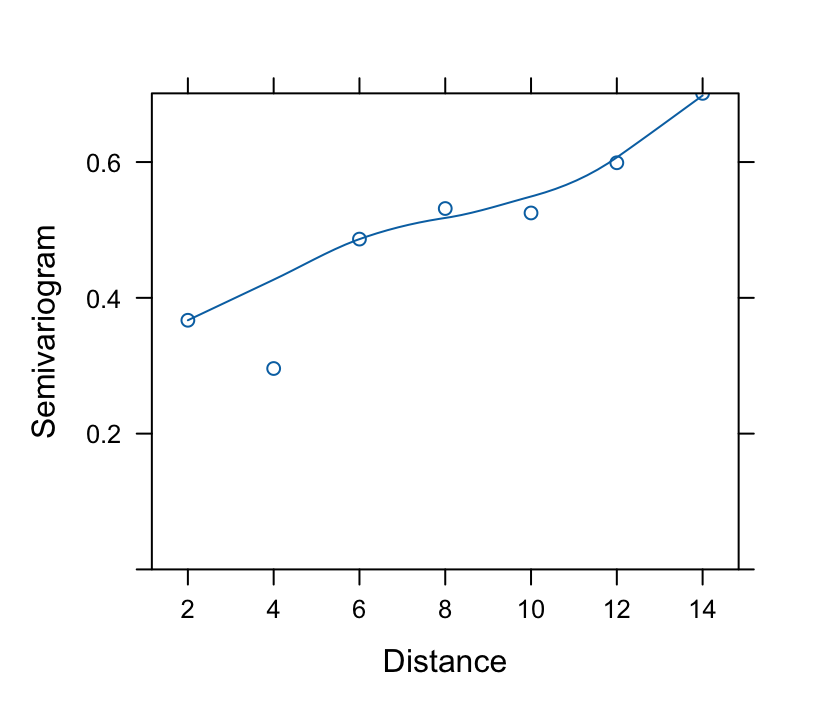
## Checking Model Fit
`r mrg(sound("gls-7"))`
* Constant variance assumption: usual residual plots `r ipacue()`
* Normality assumption: usual qq residual plots
* Correlation pattern: **Variogram**
+ Estimate correlations of all possible pairs of residuals at
different time points
+ Pool all estimates at same absolute difference in time $s$
+ Variogram is a plot with $y = 1 - \hat{h}(s, \rho)$ vs. $s$ on
the $x$-axis
+ Superimpose the theoretical variogram assumed by the model
## `R` Software
`r mrg(sound("gls-8"))`
* Nonlinear mixed effects model package of Pinheiro \& Bates `r ipacue()`
* For linear models, fitting functions are
+ `lme` for mixed effects models
+ `gls` for generalized least squares without random effects
* For this version the rms package has `Gls` so that many
features of rms can be used:
+ **`anova`**: all partial Wald tests, test of linearity, pooled tests
+ **`summary`**: effect estimates (differences in $\hat{Y}$) and
confidence limits, can be plotted
+ **`plot, ggplot, plotp`**: continuous effect plots
+ **`nomogram`**: nomogram
+ **`Function`**: generate `R` function code for fitted model
+ **`latex`**: \LaTeX\ representation of fitted model
In addition, `Gls` has a bootstrap option (hence you do not
use rms's `bootcov` for `Gls` fits).<br>
To get regular `gls` functions named `anova` (for
likelihood ratio tests, AIC, etc.) or `summary` use
`anova.gls` or `summary.gls`
* `nlme` package has many graphics and fit-checking functions
* Several functions will be demonstrated in the case study
## Case Study
`r mrg(sound("gls-9"))`
Consider the dataset in Table~6.9 of
Davis[davis-repmeas, pp. 161-163] from a multi-center, randomized
controlled trial of botulinum toxin type B (BotB) in patients with cervical
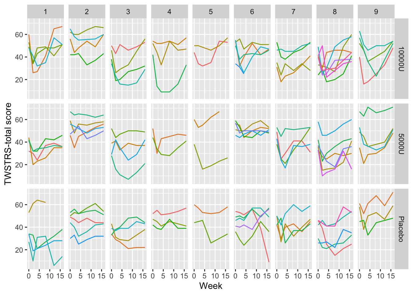
dystonia from nine U.S. sites.
* Randomized to placebo ($N=36$), 5000 units of BotB ($N=36$), `r ipacue()`
10,000 units of BotB ($N=37$)
* Response variable: total score on Toronto Western Spasmodic
Torticollis Rating Scale (TWSTRS), measuring severity, pain, and
disability of cervical dystonia (high scores mean more impairment)
* TWSTRS measured at baseline (week 0) and weeks 2, 4, 8, 12, 16
after treatment began
* Dataset `cdystonia` from web site
### Graphical Exploration of Data
```{r spaghetti,h=5,w=7,cap='Time profiles for individual subjects, stratified by study site and dose'}
#| label: fig-long-spaghetti
require(rms)
require(data.table)
options(prType='html')    # for model print, summary, anova, validate
getHdata(cdystonia)
setDT(cdystonia)          # convert to data.table
cdystonia[, uid := paste(site, id)]   # unique subject ID

# Tabulate patterns of subjects' time points
g <- function(w) paste(sort(unique(w)), collapse=' ')
cdystonia[, table(tapply(week, uid, g))]
# Plot raw data, superposing subjects
xl <- xlab('Week'); yl <- ylab('TWSTRS-total score')
ggplot(cdystonia, aes(x=week, y=twstrs, color=factor(id))) +
       geom_line() + xl + yl + facet_grid(treat ~ site) +
       guides(color=FALSE)
```
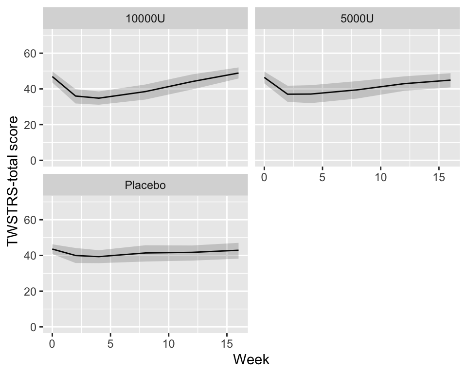
```{r quartiles,cap='Quartiles of `TWSTRS` stratified by dose',w=5,h=4}
#| label: fig-long-quartiles
# Show quartiles
g <- function(x) {
  k <- as.list(quantile(x, (1 : 3) / 4, na.rm=TRUE))
  names(k) <- .q(Q1, Q2, Q3)
  k
}
cdys <- cdystonia[, g(twstrs), by=.(treat, week)]
ggplot(cdys, aes(x=week, y=Q2)) + xl + yl + ylim(0, 70) +
  geom_line() + facet_wrap(~ treat, nrow=2) +
  geom_ribbon(aes(ymin=Q1, ymax=Q3), alpha=0.2)
```
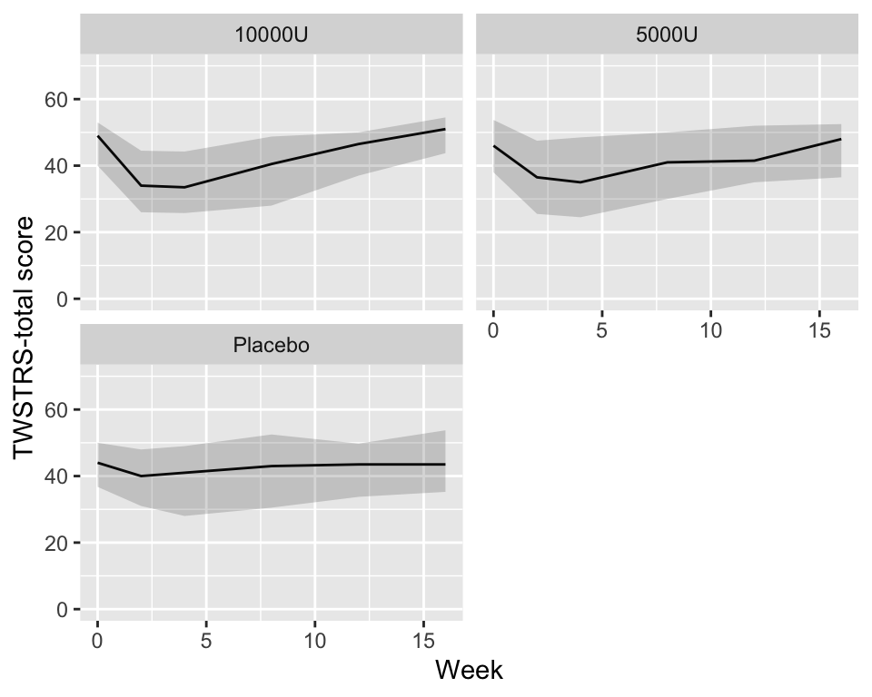
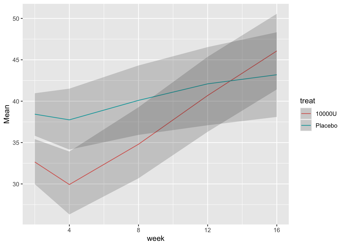
```{r bootcls,cap='Mean responses and nonparametric bootstrap 0.95 confidence limits for population means, stratified by dose',w=5,h=4}
#| label: fig-long-bootcls
# Show means with bootstrap nonparametric CLs
cdys <-  cdystonia[, as.list(smean.cl.boot(twstrs)),
                   by = list(treat, week)]
ggplot(cdys, aes(x=week, y=Mean)) + xl + yl + ylim(0, 70) +
  geom_line() + facet_wrap(~ treat, nrow=2) +
  geom_ribbon(aes(x=week, ymin=Lower, ymax=Upper), alpha=0.2)
```
#### Model with $Y_{i0}$ as Baseline Covariate
```{r}
baseline <- cdystonia[week == 0]
baseline[, week := NULL]
setnames(baseline, 'twstrs', 'twstrs0')
followup <- cdystonia[week > 0, .(uid, week, twstrs)]
setkey(baseline, uid)
setkey(followup, uid, week)
both     <- Merge(baseline, followup, id = ~ uid)
# Remove person with no follow-up record
both     <- both[! is.na(week)]
dd       <- datadist(both)
options(datadist='dd')
```
### Using Generalized Least Squares
`r mrg(sound("gls-10"))`
We stay with baseline adjustment and use a variety of correlation `r ipacue()`
structures, with constant variance. Time is modeled as a restricted
cubic spline with 3 knots, because there are only 3 unique interior
values of `week`.
```{r k}
```
AIC computed above is set up so that smaller values are best. From
this the continuous-time AR1 and exponential structures are tied for
the best. For the remainder of the analysis use `corCAR1`,
using `Gls`. [ @kes98com did a simulation study to study the reliability of AIC for selecting the correct covariance structure in repeated measurement models. In choosing from among 11 structures, AIC selected the correct structure 47% of the time. @gur11avo demonstrated that fixed effects in a mixed effects model can be biased, independent of sample size, when the specified covariate matrix is more restricted than the true one.]{.aside}
```{r l}
```
$\hat{\rho} = 0.8672$, the estimate of the correlation between two `r ipacue()`
measurements taken one week apart on the same subject. The estimated
correlation for measurements 10 weeks apart is $0.8672^{10} = 0.24$.
```{r fig-long-variogram,fig.cap='Variogram, with assumed correlation pattern superimposed',h=3.75,w=4.25}
#| label: fig-long-variogram
```
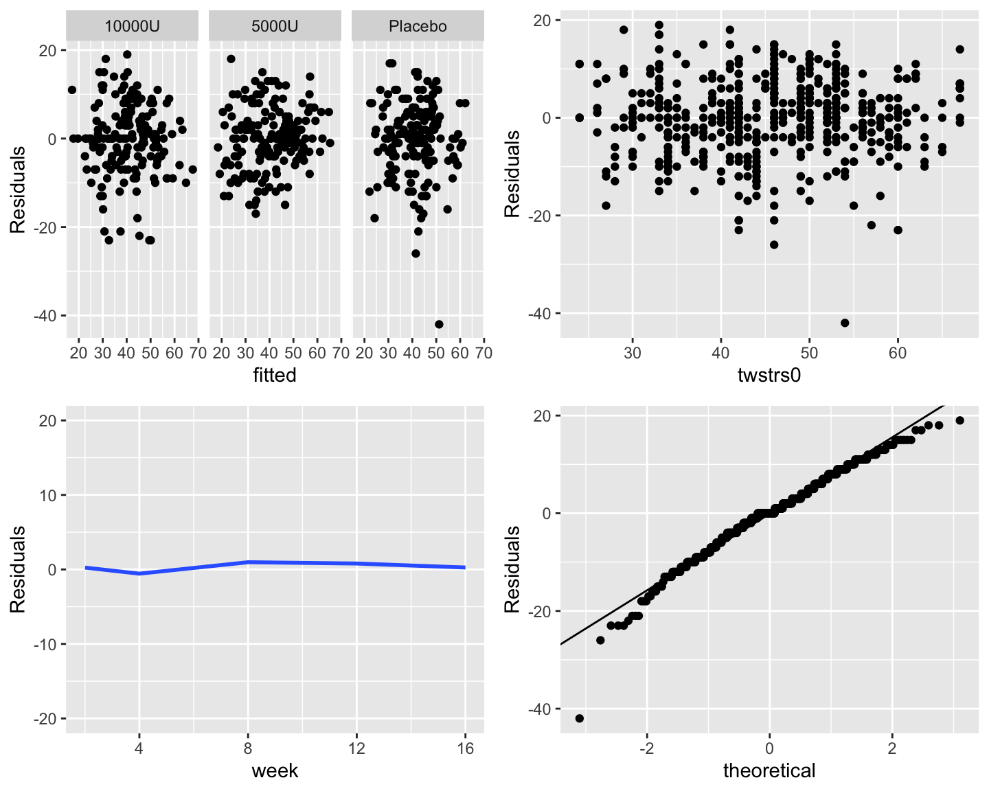
Check constant variance and normality assumptions: `r ipacue()`
```{r fig-long-resid,h=6,w=7.5,cap='Three residual plots to check for absence of trends in central tendency and in variability. Upper right panel shows the baseline score on the $x$-axis. Bottom left panel shows the mean $\\pm 2\\times$ SD. Bottom right panel is the QQ plot for checking normality of residuals from the GLS fit.'}
#| label: fig-long-resid
```
Now get hypothesis tests, estimates, and graphically interpret the
model.
`r mrg(sound("gls-11"))`
```{r m}
```
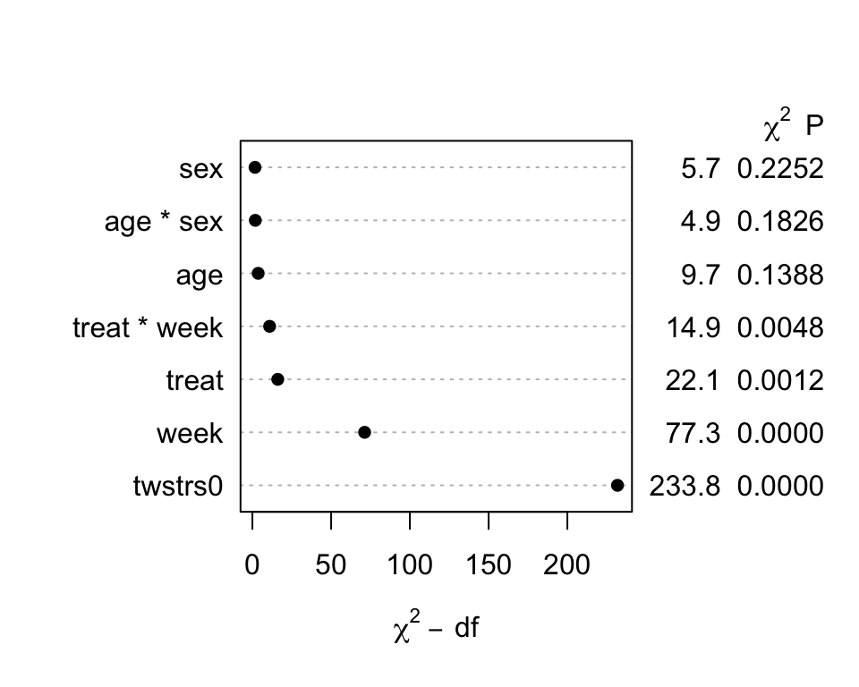
```{r fig-long-anova,cap='Results of `anova.rms` from generalized least squares fit with continuous time AR1 correlation structure',w=5,h=4}
#| label: fig-long-anova
```
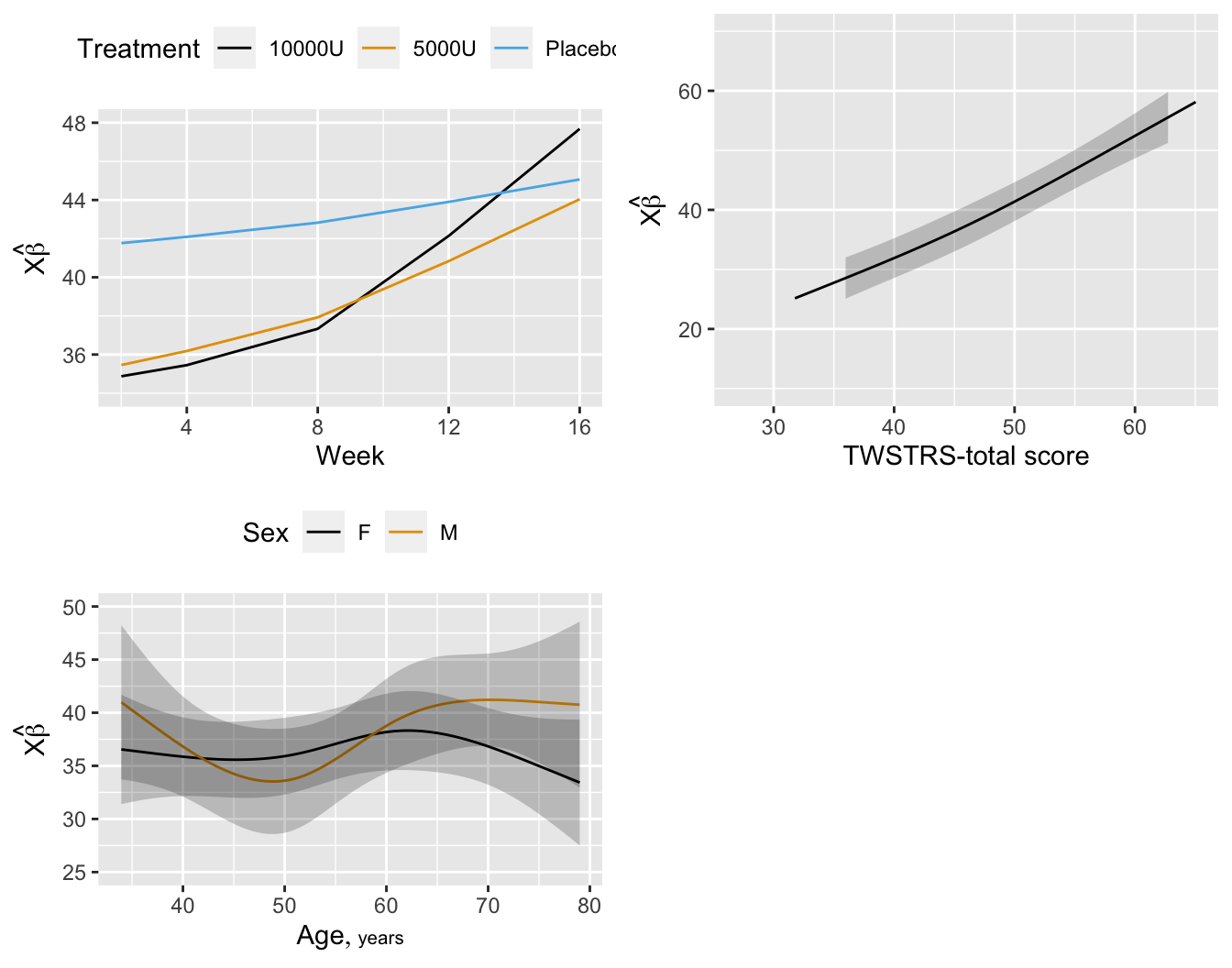
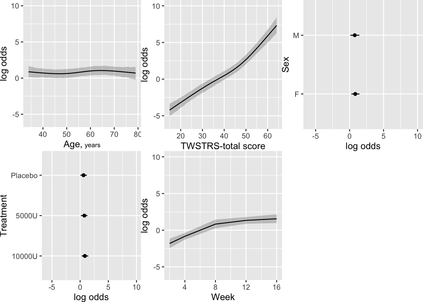
```{r fig-long-pleffects,h=5.5,w=7,cap='Estimated effects of time, baseline `TWSTRS`, age, and sex'}
#| label: fig-long-pleffects
```
```{r o}
```
```{r p}
```
```{r q}
```
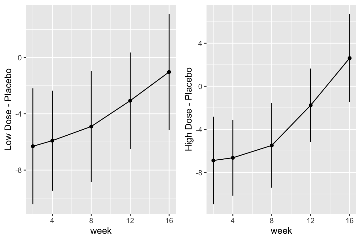
```{r fig-long-contrasts,h=4,w=6,cap='Contrasts and 0.95 confidence limits from GLS fit'}
#| label: fig-long-contrasts
```
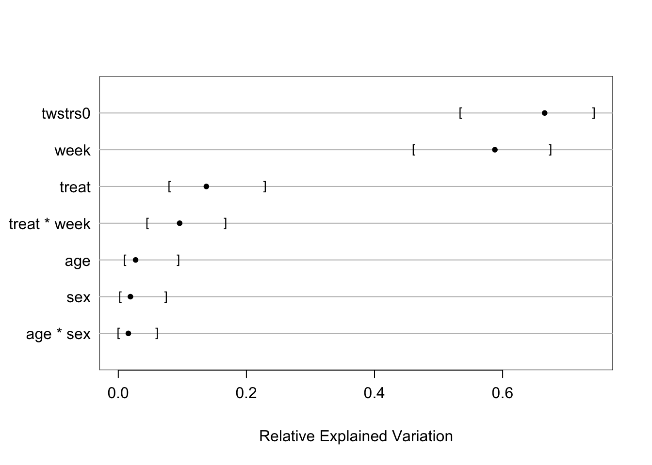
Although multiple d.f. tests such as total treatment effects or `r ipacue()`
treatment $\times$ time interaction tests are comprehensive, their
increased degrees of freedom can dilute power. In a treatment
comparison, treatment contrasts at the last time point (single
d.f. tests) are often of major interest. Such contrasts are
informed by all the measurements made by all subjects (up until
dropout times) when a smooth time trend is assumed.
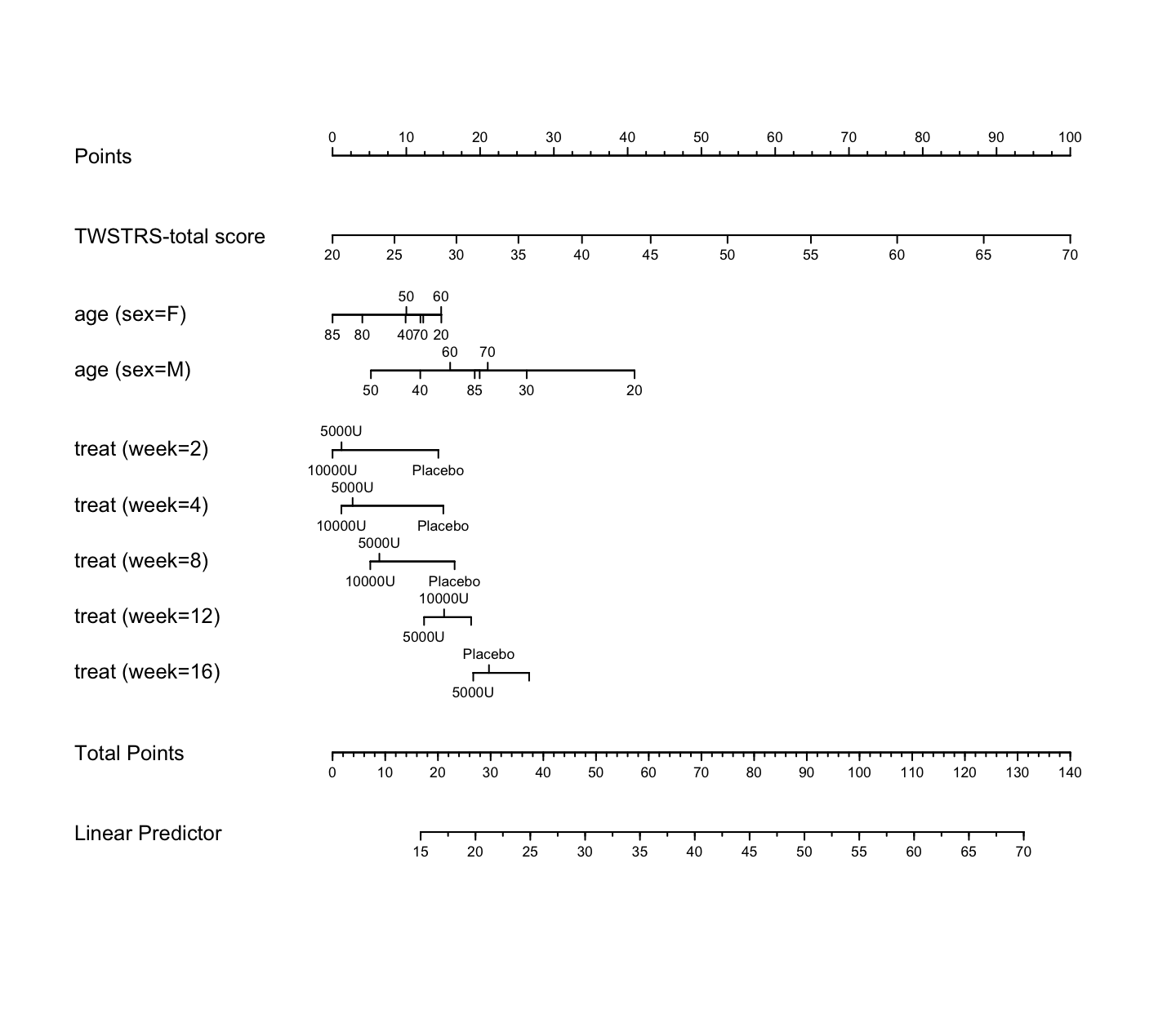
```{r nomogram,h=6.5,w=7.5,cap='Nomogram from GLS fit. Second axis is the baseline score.'}
#| label: fig-long-nomogram
n <- nomogram(a, age=c(seq(20, 80, by=10), 85))
plot(n, cex.axis=.55, cex.var=.8, lmgp=.25)  # Figure (*\ref{fig:longit-nomogram}*)
```
### Bayesian Proportional Odds Random Effects Model {#sec-long-bayes-re}
* Develop a $y$-transformation invariant longitudinal model `r ipacue()`
* Proportional odds model with no grouping of TWSTRS scores
* Bayesian random effects model
* Random effects Gaussian with exponential prior distribution for
its SD, with mean 1.0
* Compound symmetry correlation structure
* Demonstrates a large amount of patient-to-patient intercept variability
```{r bayesfit}
```
```{r bayesfit2}
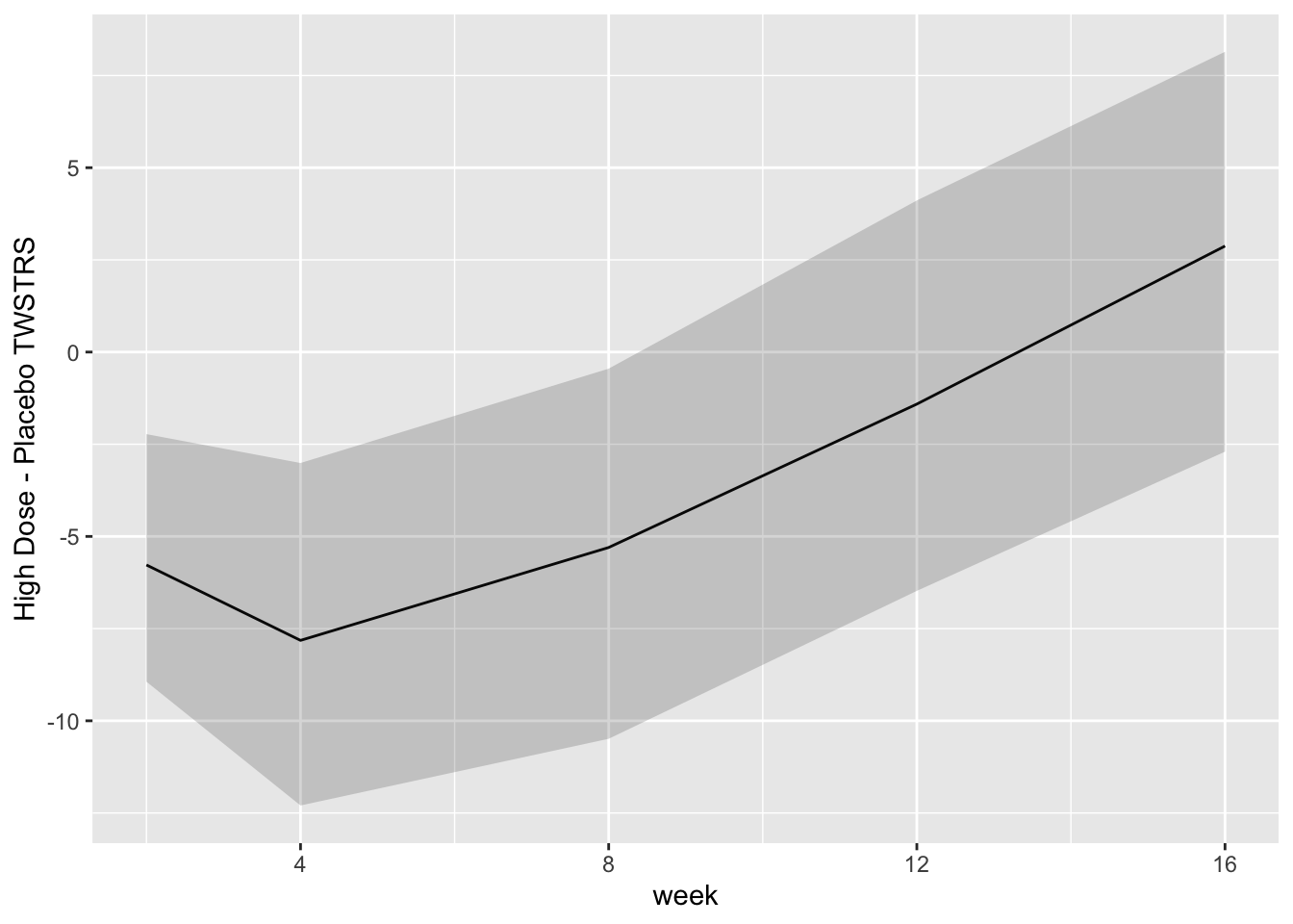
```
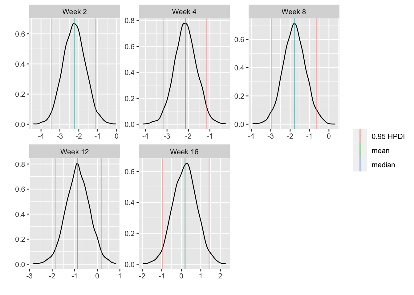
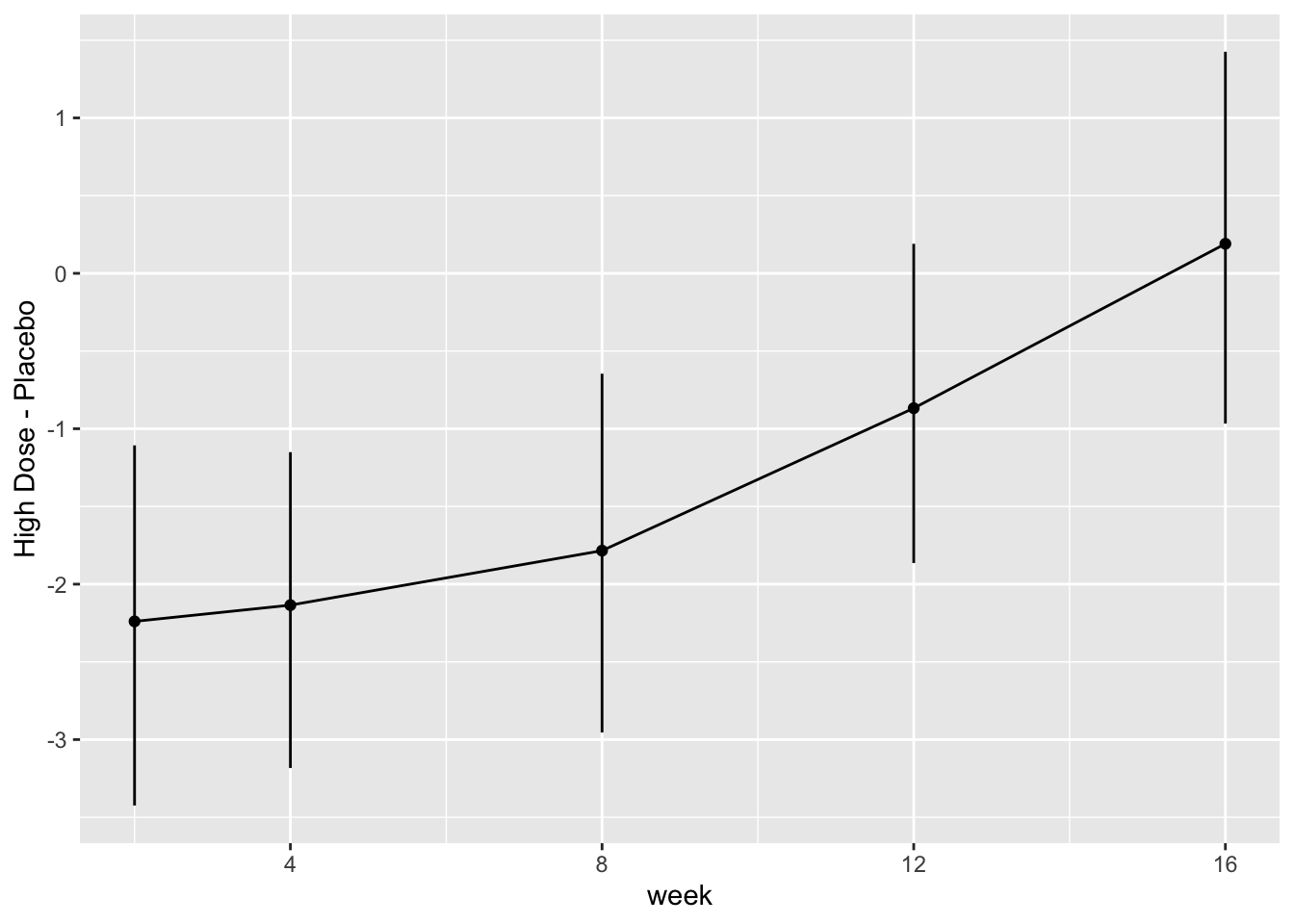
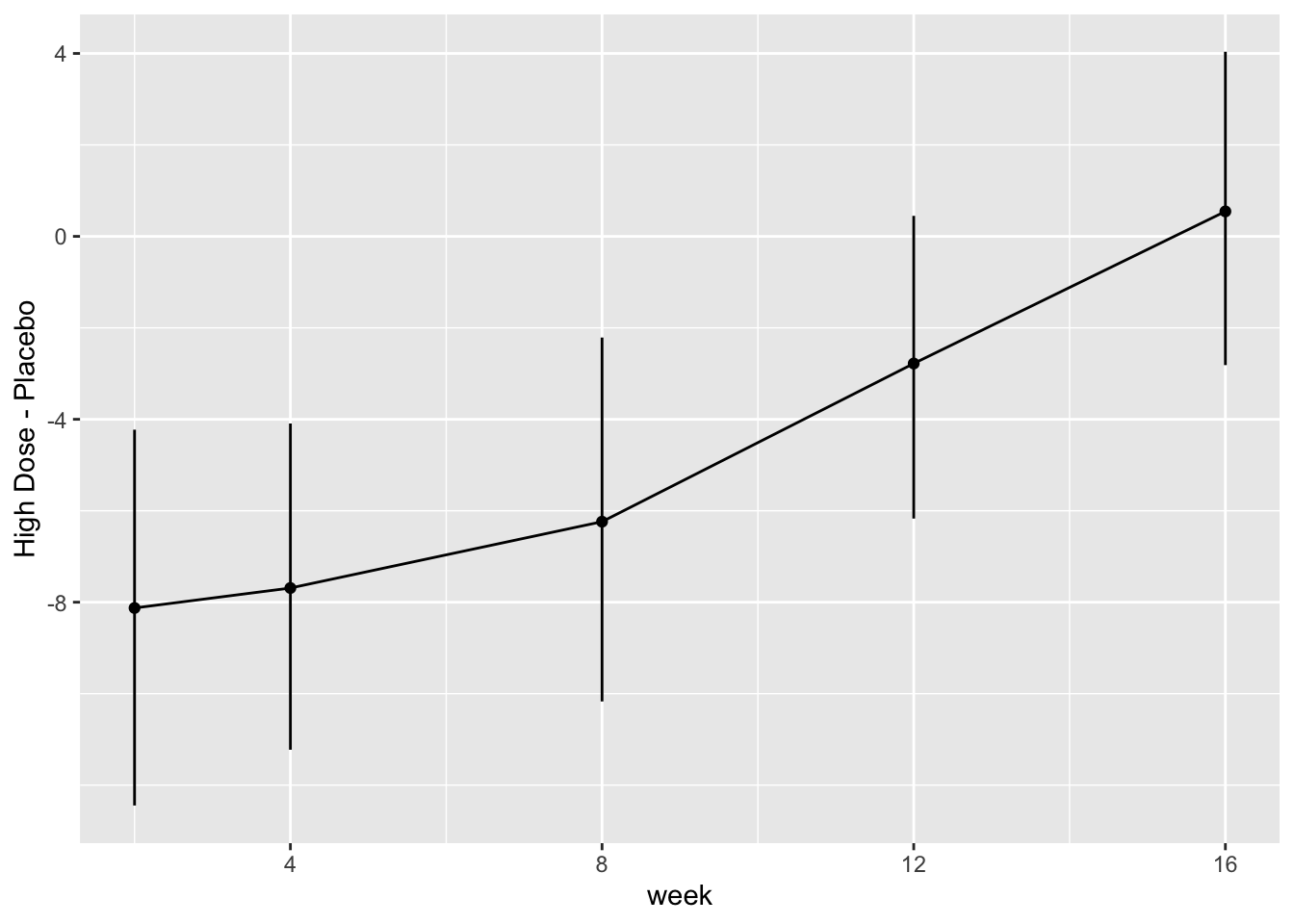
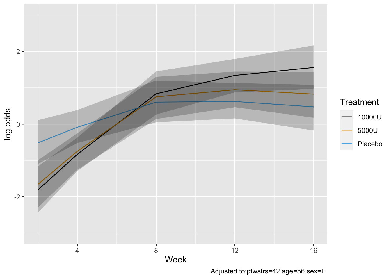
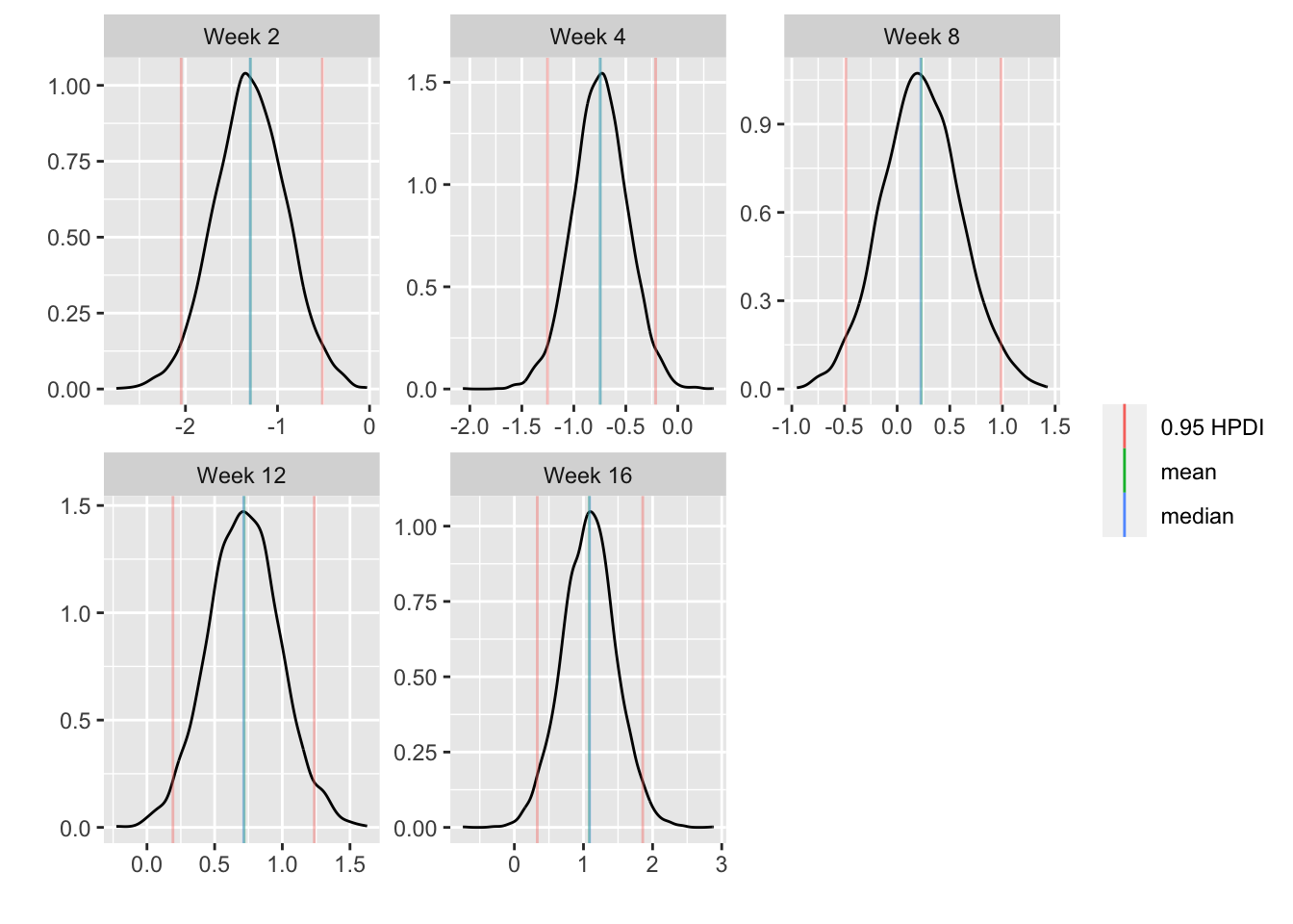
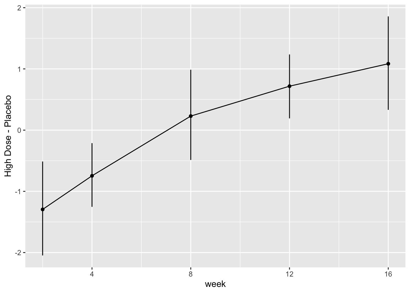
* Show the final graphic (high dose:placebo contrast as function of time `r ipacue()`
* Intervals are 0.95 highest posterior density intervals
* $y$-axis: log-odds ratio
```{r bayesfit3}
```
```{r bayesfit4}
```
For each posterior draw compute the difference in means and get an
exact (to within simulation error) 0.95 highest posterior density
intervals for these differences.
```{r bayesfit5,w=7,h=3.75}
```
```{r bayesfit6}
```
### Bayesian Markov Semiparametric Model {#sec-long-bayes-markov}
* First-order Markov model `r ipacue()`
* Serial correlation induced by Markov model is similar to AR(1)
which we already know fits these data
* Markov model is more likely to fit the data than the random
effects model, which induces a compound symmetry correlation structure
* Models state transitions
* PO model at each visit, with Y from previous visit conditioned
upon just like any covariate
* Need to uncondition (marginalize) on previous Y to get the
time-response profile we usually need
* Semiparametric model is especially attractive because one can
easily "uncondition" a discrete Y model, and the distribution of Y
for control subjects can be any shape
* Let measurement times be $t_{1}, t_{2}, \dots, t_{m}$, and the measurement for a subject at time $t$ be denoted $Y(t)$
* First-order Markov model:
\begin{array}{ccc}
\Pr(Y(t_{i}) \geq y | X, Y(t_{i-1})) &=& \mathrm{expit}(\alpha_{y} + X\beta\\
&+& g(Y(t_{i-1}), t_{i}, t_{i} - t_{i-1}))
\end{array}
* $g$ involves any number of regression coefficients for a main effect of $t$, the main effect of time gap $t_{i} - t_{i-1}$ if this is not collinear with absolute time, a main effect of the previous state, and interactions between these
* Examples of how the previous state may be modeled in $g$:
+ linear in numeric codes for $Y$
+ spline function in same
+ discontinuous bi-linear relationship where there is a slope for in-hospital outcome severity, a separate slope for outpatient outcome severity, and an intercept jump at the transition from inpatient to outpatient (or _vice versa_)
* Markov model is quite flexible in handling time trends and serial correlation patterns
* Can allow for irregular measurement times:<br> [hbiostat.org/stat/irreg.html](https://hbiostat.org/stat/irreg.html)
Fit the model and run standard Stan diagnostics.
```{r mark1,h=6,w=7.5}
```
Note that posterior sampling is much more efficient without random effects.
```{r mark2}
```
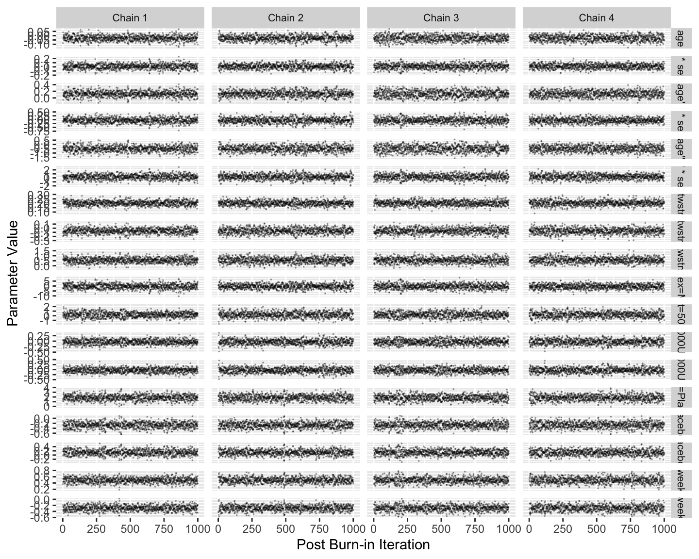
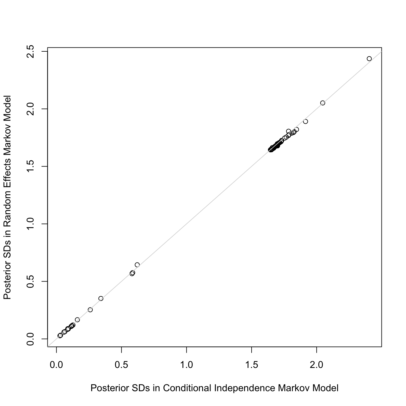
Let's add subject-level random effects to the model. Smallness of the
standard deviation of the random effects provides support for the
assumption of conditional independence that we like to make for Markov
models and allows us to simplify the model by omitting random effects.
```{r mark3}
```
```{r mark4}
```
The random effects SD is only 0.11 on the logit scale. Also, the
standard deviations of all the regression parameter posterior distributions are
virtually unchanged with the addition of random effects:
```{r mark4r,w=7,h=7}
```
So we will use the model omitting random effects.
Show the partial effects of all the predictors, including the effect
of the previous measurement of TWSTRS. Also compute high dose:placebo
treatment contrasts on these conditional estimates.
```{r mark5}
```
```{r mark5b}
```
Using posterior means for parameter values, compute the probability
that at a given week `twstrs` will be $\geq 40$ when at the
previous visit it was 40. Also show the conditional mean `twstrs`
when it was 40 at the previous visit.
```{r mark6}
```
```{r mark6b}
```
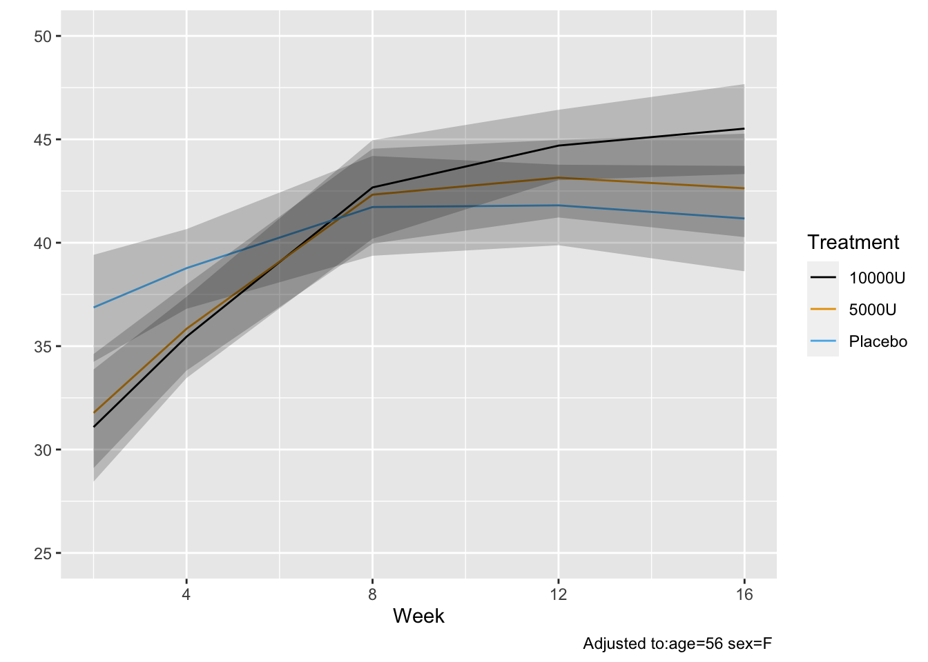
* Semiparametric models provide not only estimates of tendencies of Y `r ipacue()`
but also estimate the whole distribution of Y
* Estimate the entire conditional distribution of Y at week 12 for
high-dose patients having `TWSTRS`=42 at week 8
* Other covariates set to median/mode
* Use posterior mean of all the cell probabilities
* Also show pointwise 0.95 highest posterior density intervals
* To roughly approximate simultaneous confidence bands make the
pointwise limits sum to 1 like the posterior means do
```{r mark6c}
```
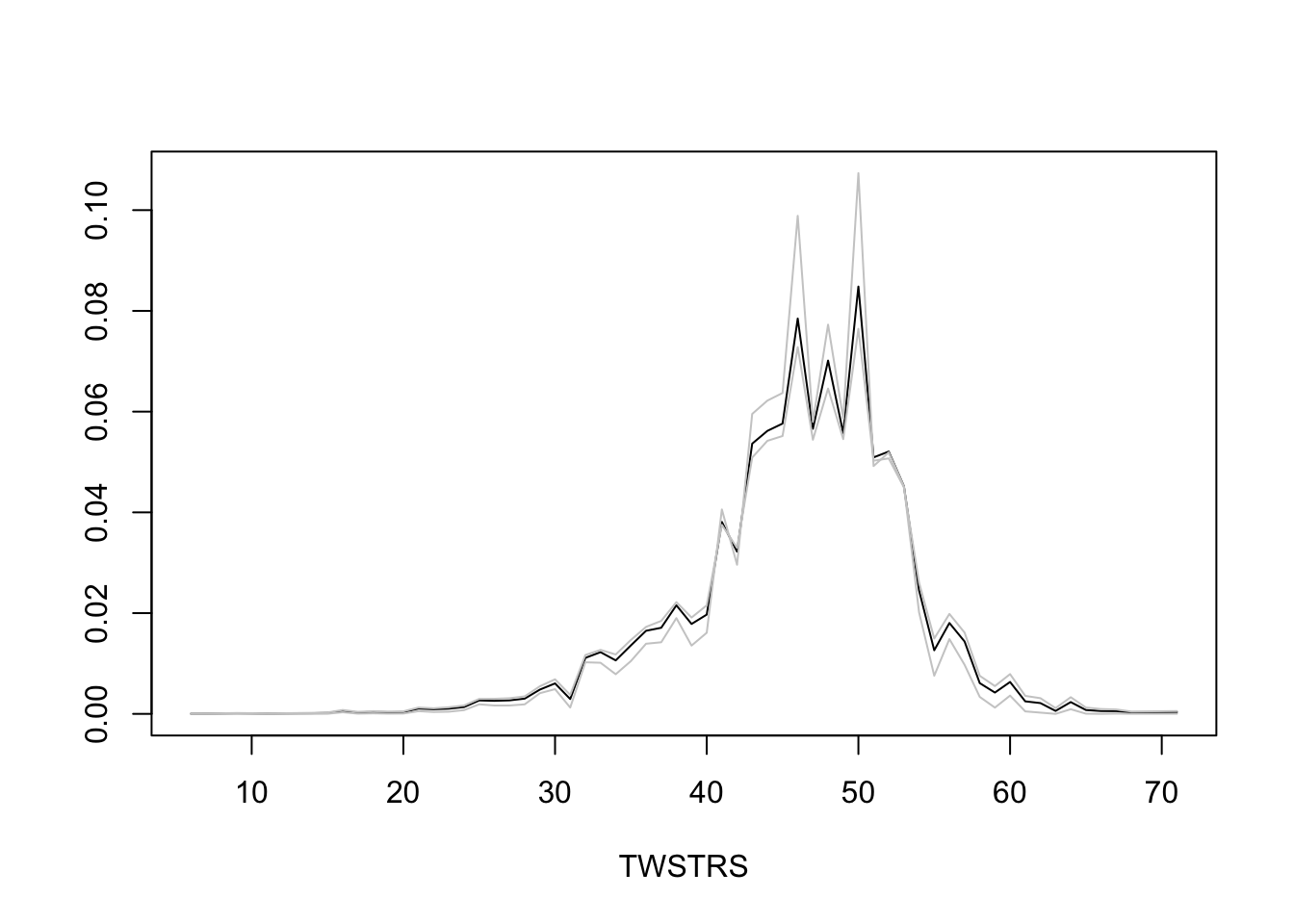
* Repeat this showing the variation over 5 posterior draws `r ipacue()`
```{r mark6d}
```
* Turn to marginalized (unconditional on previous `twstrs`) `r ipacue()`
quantities
* Capitalize on PO model being a multinomial model, just with PO
restrictions
* Manipulations of conditional probabilities to get the
unconditional probability that `twstrs`=y doesn't need to know
about PO
* Compute all cell probabilities and use the law
of total probability recursively
$$\Pr(Y_{t} = y | X) = \sum_{j=1}^{k} \Pr(Y_{t} = y | X, Y_{t-1} = j) \Pr(Y_{t-1} = j | X)$$
* `predict.blrm` method with `type='fitted.ind'` computes
the needed conditional cell probabilities, optionally for all
posterior draws at once
* Easy to get highest posterior density intervals for derived
parameters such as unconditional probabilities or unconditional
means
* `Hmisc` package `soprobMarkovOrdm` function (in version
4.6) computes an array of all the state occupancy probabilities for
all the posterior draws
```{r mark7}
```
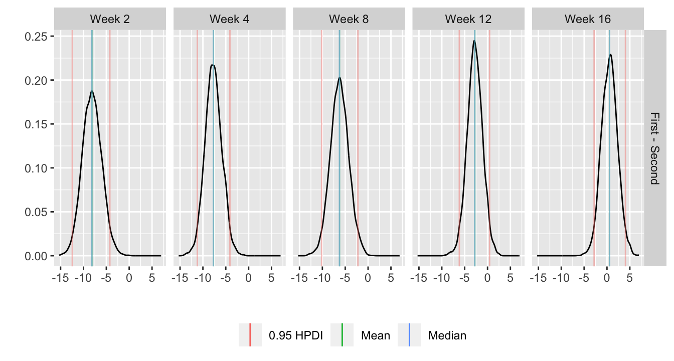
* Use the same posterior draws of unconditional probabilities of all `r ipacue()`
values of TWSTRS to get the posterior distribution of differences in
mean TWSTRS between high and low dose
```{r mark8}
```
* Get posterior mean of all cell probabilities estimates at week 12 `r ipacue()`
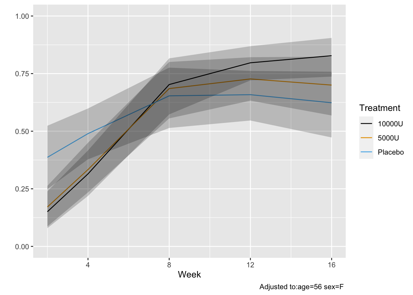
* Distribution of TWSTRS conditional high dose, median age, mode sex
* Not conditional on week 8 value
```{r mark9}
```
## Study Questions
**Section 7.2**
1. When should one model the time-response profile using discrete time?
**Section 7.3**
1. What makes generalized least squares and mixed effect models
relatively robust to non-completely-random dropouts?
1. What does the last observation carried forward method always violate?
**Section 7.4**
1. Which correlation structure do you expect to fit the data when there are rapid repetitions over a short time span? When the follow-up time span is very long?
**Section 7.8**
1. What can go wrong if many correlation structures are tested in one dataset?
1. In a longitudinal intervention study, what is the most typical comparison of interest? Is it best to borrow information in estimating this contrast?
```{r echo=FALSE}
saveCap('07')
```