```{r include=FALSE}
require(Hmisc)
options(qproject='rms', prType='html')
require(qreport)
getRs('qbookfun.r')
hookaddcap()
knitr::set_alias(w = 'fig.width', h = 'fig.height', cap = 'fig.cap', scap ='fig.scap')
```
# Case Study in Parametric Survival Modeling and Model Approximation {#sec-psmcase}
`r mrg(sound("psm-case-1"))`
**Data source**: Random sample of 1000 patients from Phases I \& II
of SUPPORT (Study to Understand Prognoses Preferences Outcomes and
Risks of Treatment, funded by the Robert Wood Johnson Foundation). See @kna95sup. The dataset is available from [hbiostat.org/data](https://hbiostat.org/data).
* Analyze acute disease subset of SUPPORT (acute respiratory `r ipacue()`
failure, multiple organ system failure, coma) --- the shape
of the survival curves is different between acute and chronic disease
categories
* Patients had to survive until day 3 of the study to qualify
* Baseline physiologic variables measured during day 3
## Descriptive Statistics
Create a variable `acute` to flag categories of
interest; print univariable descriptive statistics.
```{r results='asis'}
require(rms)
options(prType='html')     # for print, summary, anova
getHdata(support)          # Get data frame from web site
acute <- support$dzclass %in% c('ARF/MOSF','Coma')
des <- describe(support[acute,])
sparkline::sparkline(0)    # load sparkline dependencies
maketabs(print(des, 'both'), wide=TRUE, initblank=TRUE)
```
`r ipacue()`
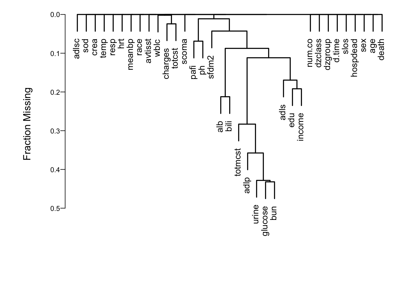
```{r naclus,h=5,w=7,cap='Cluster analysis showing which predictors tend to be missing on the same patients',scap='Cluster analysis of missingness in SUPPORT'}
#| label: fig-psmcase-naclus
spar(ps=11)
# Show patterns of missing data
plot(naclus(support[acute,]))
```
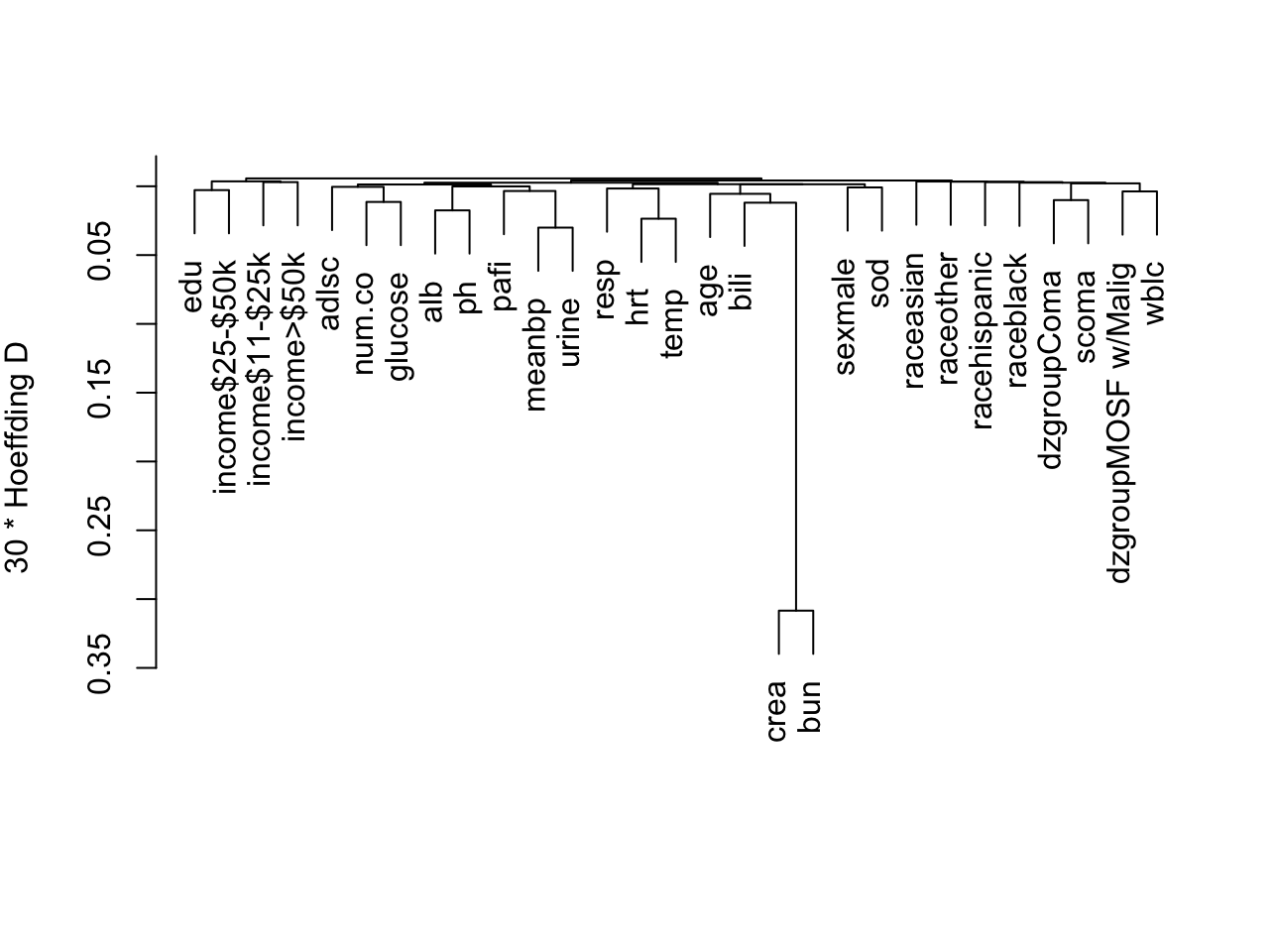
Show associations between predictors using a general non-monotonic
measure of dependence (Hoeffding $D$). `r ipacue()`
```{r varclus,w=6.7,cap='Hierarchical clustering of potential predictors using Hoeffding $D$ as a similarity measure. Categorical predictors are automatically expanded into dummy variables.',scap='Clustering of predictors in SUPPORT using Hoeffding $D$'}
#| label: fig-psmcase-varclus
ac <- support[acute,]
ac$dzgroup <- ac$dzgroup[drop=TRUE]    # Remove unused levels
vc <- varclus(~ age+sex+dzgroup+num.co+edu+income+scoma+race+
              meanbp+wblc+hrt+resp+temp+pafi+alb+bili+crea+sod+
              ph+glucose+bun+urine+adlsc, data=ac, sim='hoeffding')
plot(vc)
```
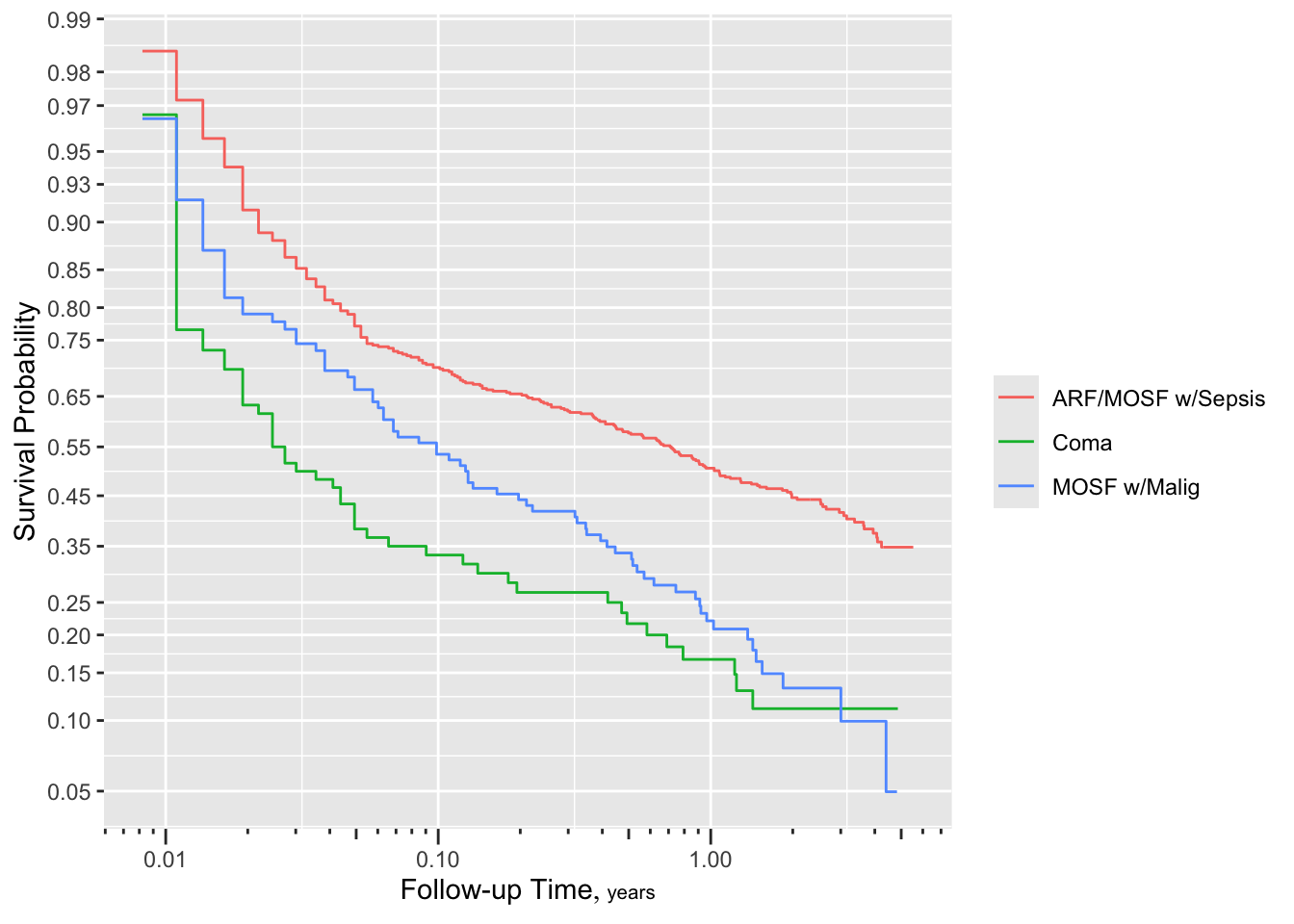
## Checking Adequacy of Log-Normal Accelerated Failure Time Model {#sec-psmcase-lognorm-gof}
`r mrg(sound("psm-case-2"))`
```{r nikm,cap='$\\Phi^{-1}(S_{\text{KM}}(t))$ stratified by `dzgroup`. Linearity and semi-parallelism indicate a reasonable fit to the log-normal accelerated failure time model with respect to one predictor.',scap='$\\Phi^{-1}(S_{\text{KM}}(t))$ stratified by `dzgroup`'}
#| label: fig-psmcase-nikm
dd <- datadist(ac)
# describe distributions of variables to rms
options(datadist='dd')

# Generate right-censored survival time variable
ac <- upData(ac, print=FALSE,
  years = d.time/365.25,
  labels = c(years = 'Follow-up Time'),
  units = c(years = 'Year'))
ac$S <- with(ac,  Surv(years, death))

# Show normal inverse Kaplan-Meier estimates
# stratified by dzgroup
ggplot(npsurv(S ~ dzgroup, data=ac), conf='none',
       trans='probit', logt=TRUE)
```
<!-- ggplot is new -->
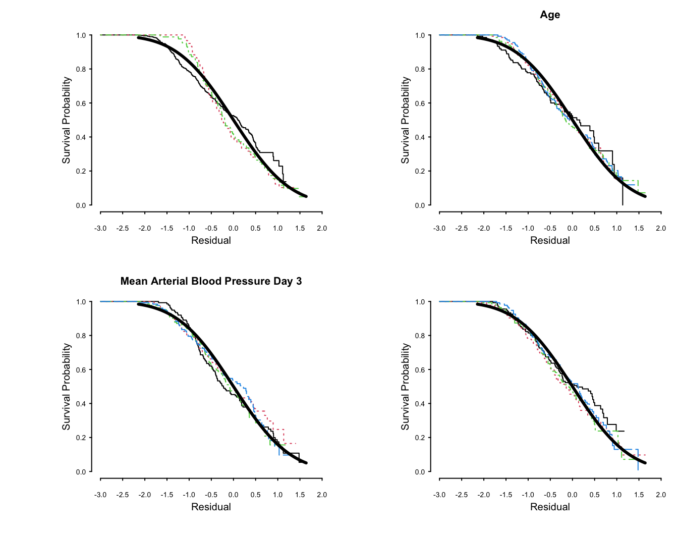
More stringent assessment of log-normal assumptions: check
distribution of residuals from an adjusted model: `r ipacue()`
```{r lognorm-resid, w=7, h=5.5, mfrow=c(2,2),cap='Kaplan-Meier estimates of distributions of normalized, right-censored residuals from the fitted log-normal survival model. Residuals are stratified by important variables in the model (by quartiles of continuous variables), plus a random variable to depict the natural variability (in the lower right plot). Theoretical standard Gaussian distributions of residuals are shown with a thick solid line. The upper left plot is with respect to disease group.',scap='Distributions of residuals from log-normal model'}
#| label: fig-psmcase-lognorm-resid
spar(mfrow=c(2,2), ps=8, top=1, lwd=1)
f <- psm(S ~ dzgroup + rcs(age,5) + rcs(meanbp,5),
               dist='lognormal', y=TRUE, data=ac)
r <- resid(f)
with(ac, {
  survplot(r, dzgroup, label.curve=FALSE)
  survplot(r, age,     label.curve=FALSE)
  survplot(r, meanbp,  label.curve=FALSE)
  survplot(r, runif(length(age)), label.curve=FALSE)
} )
```
The fit for `dzgroup` is not great but overall fit is good.
Remove from consideration predictors that are missing in $> 0.2$ of
the patients. Many of these were only collected for the second phase
of SUPPORT.
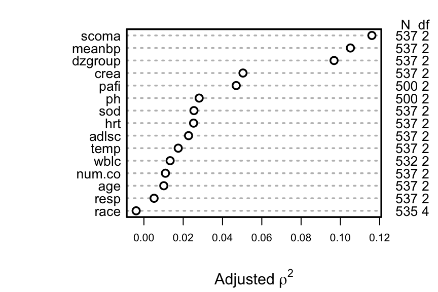
Of those variables to be included in the model, find which
`r mrg(sound("psm-case-3"))`
ones have enough potential predictive power to justify allowing for
nonlinear relationships or multiple categories, which spend more d.f.
For each variable compute Spearman $\rho^2$
based on multiple linear regression of rank($x$), rank($x$)$^2$ and
the survival time, truncating survival time at the shortest follow-up
for survivors (356 days). This rids the data of censoring but creates
many ties at 356 days.
```{r spearman, w=4.5, cap='Generalized Spearman $\\rho^2$ rank correlation between predictors and truncated survival time'}
#| label: fig-psmcase-spearman
#| fig-height: 3
spar(top=1, ps=10, rt=3)
ac <- upData(ac, print=FALSE,
  shortest.follow.up = min(d.time[death==0], na.rm=TRUE),
  d.timet            = pmin(d.time, shortest.follow.up))

w <- spearman2(d.timet ~ age + num.co + scoma + meanbp +
             hrt + resp + temp + crea + sod + adlsc +
             wblc + pafi + ph + dzgroup + race, p=2, data=ac)
plot(w, main='')
```
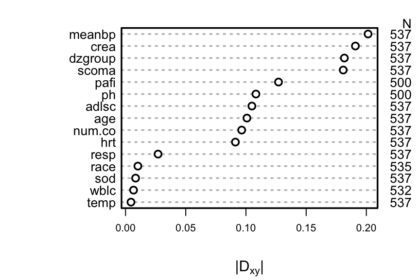
A better approach is to use the complete information in the failure `r ipacue()`
and censoring times by computing Somers' $D_{xy}$ rank correlation
allowing for censoring.
```{r rcorrcens, w=4.5, cap='Somers\' $D_{xy}$ rank correlation between predictors and original survival time. For `dzgroup` or `race`, the correlation coefficient is the maximum correlation from using a dummy variable to represent the most frequent or one to represent the second most frequent category.',scap='Somers\' $D_{xy}$ rank correlation between predictors and original survival time'}
#| label: fig-psmcase-rcorrcens
#| fig-height: 3
spar(top=1, ps=10, rt=3)
w <- rcorrcens(S ~ age + num.co + scoma + meanbp + hrt + resp +
               temp + crea + sod + adlsc + wblc + pafi + ph +
               dzgroup + race, data=ac)
plot(w, main='')
```
```{r }
# Compute number of missing values per variable
sapply(ac[.q(age,num.co,scoma,meanbp,hrt,resp,temp,crea,sod,adlsc,
             wblc,pafi,ph)], function(x) sum(is.na(x)))
# Can also do naplot(naclus(support[acute,]))
# Can also use the Hmisc naclus and naplot functions to do this
# Impute missing values with normal or modal values
ac <- upData(ac, print=FALSE,
  wblc.i = impute(wblc, 9),
  pafi.i = impute(pafi, 333.3),
  ph.i   = impute(ph,   7.4),
  race2  = ifelse(is.na(race), 'white',
                  ifelse(race != 'white', 'other', 'white')) )
dd <- datadist(ac)
```
Do a formal redundancy analysis using more than pairwise associations, `r ipacue()`
and allow for non-monotonic transformations in predicting each
predictor from all other predictors. This analysis requires missing
values to be imputed so as to not greatly reduce the sample size.
```{r }
r <- redun(~ crea + age + sex + dzgroup + num.co + scoma + adlsc + race2 +
           meanbp + hrt + resp + temp + sod + wblc.i + pafi.i + ph.i,
           data=ac, nk=4)
r
r2describe(r$scores, nvmax=4) # show top 4 strongest predictors of each var.
```
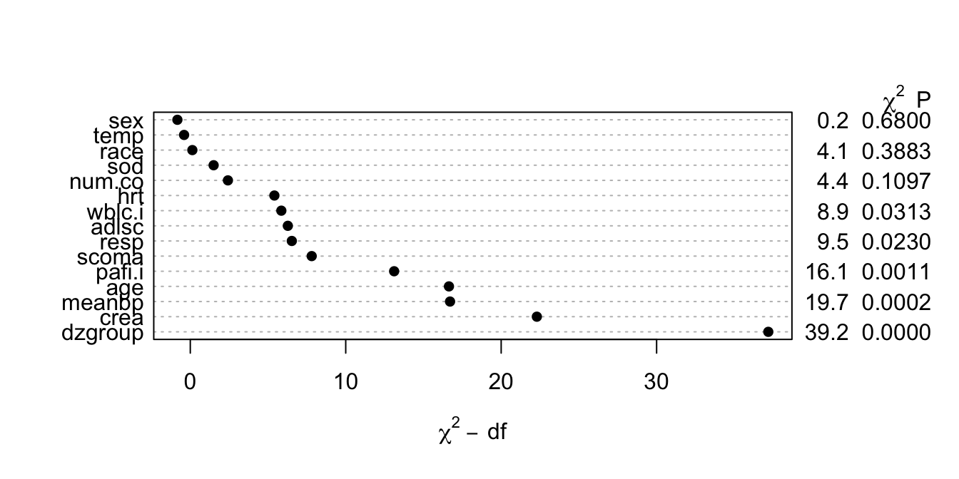
Better approach to gauging predictive potential and allocating d.f.:
* Allow all continuous variables to have a the maximum number of `r ipacue()`
knots entertained, in a log-normal survival model
* Must use imputation to avoid losing data
* Fit a "saturated" main effects model
* Makes full use of censored data
* Had to limit to 4 knots, force `scoma` to be linear, and omit
`ph.i` to avoid singularity
<!-- NEW Wald -> LR -->
```{r anovasat,cap='Partial likelihood ratio $\\chi^{2}$ statistics for association of each predictor with response from saturated main effects model, penalized for d.f.',scap='Partial $\\chi^{2}$ statistics from saturated main effects model'}
#| label: fig-psmcase-anovasat
#| fig-height: 3.5
k <- 4
f <- psm(S ~ rcs(age,k)+sex+dzgroup+pol(num.co,2)+scoma+
         pol(adlsc,2)+race+rcs(meanbp,k)+rcs(hrt,k)+rcs(resp,k)+
         rcs(temp,k)+rcs(crea,k)+rcs(sod,k)+rcs(wblc.i,k)+
         rcs(pafi.i,k), dist='lognormal', data=ac, x=TRUE, y=TRUE)
plot(anova(f, test='LR'))
```
* This figure properly blinds the analyst to the form `r ipacue()`
of effects (tests of linearity).
* Fit a log-normal survival model `r ipacue()`
with number of parameters corresponding to nonlinear effects
determined from @fig-psmcase-anovasat. For the most promising
predictors, five knots can be allocated, as there are fewer
singularity problems once less promising predictors are simplified.
**Note**: Since the audio was recorded, a bug in `psm` was fixed on 2017-03-12.
Discrimination indexes shown in the table below are correct
but the audio is incorrect for $g$ and $g_{r}$.
```{r}
f <- psm(S ~ rcs(age,5) + sex + dzgroup + num.co +
             scoma + pol(adlsc,2) + race2 + rcs(meanbp,5) +
             rcs(hrt,3) + rcs(resp,3) + temp +
             rcs(crea,4) + sod + rcs(wblc.i,3) + rcs(pafi.i,4),
         dist='lognormal', data=ac, x=TRUE, y=TRUE)
f
a <- anova(f, test='LR')
```
## Summarizing the Fitted Model
`r mrg(sound("psm-case-4"))`
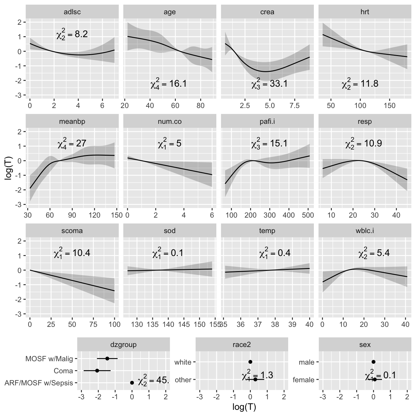
* Plot the shape of the effect of each predictor on log `r ipacue()`
survival time.
* All effects centered: can be placed on common scale
* LR $\chi^2$ statistics, penalized for d.f., plotted in descending order
```{r plot, h=7, w=7, cap='Effect of each predictor on log survival time. Predicted values have been centered so that predictions at predictor reference values are zero. Pointwise 0.95 confidence bands are also shown. As all $Y$-axes have the same scale, it is easy to see which predictors are strongest.',scap='Effect of predictors on log survival time in SUPPORT'}
#| label: fig-psmcase-plot
ggplot(Predict(f, ref.zero=TRUE), vnames='names',
       sepdiscrete='vertical', anova=a)
```
`r ipacue()`
```{r}
a
```
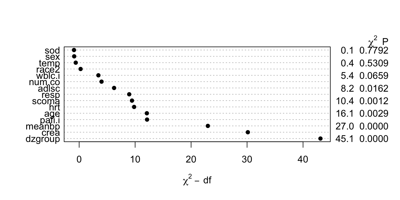
```{r anova,cap='Contribution of variables in predicting survival time in log-normal model'}
#| label: fig-psmcase-anova
#| fig-height: 3.5
plot(a)
```
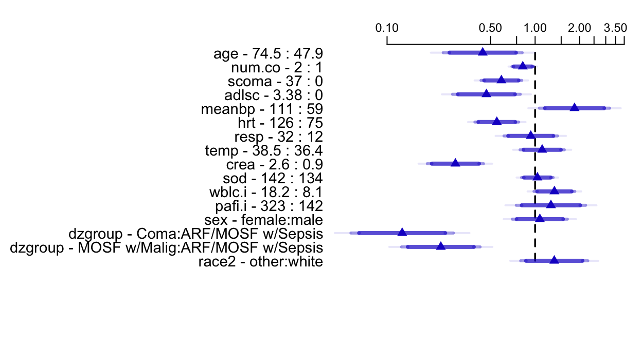
`r ipacue()`
```{r summary, w=6.5, h=3.5, cap='Estimated survival time ratios for default settings of predictors. For example, when age changes from its lower quartile to the upper quartile (47.9y to 74.5y), median survival time decreases by more than half. Different shaded areas of bars indicate different confidence levels (0.9, 0.95, 0.99).',scap='Survival time ratios from fitted log-normal model'}
#| label: fig-psmcase-summary
spar(top=1, ps=11)
options(digits=3)
plot(summary(f), log=TRUE, main='')
```
## Internal Validation of the Fitted Model Using the Bootstrap
`r mrg(sound("psm-case-5"))`
Validate indexes describing the fitted model.
```{r}
# First add data to model fit so bootstrap can re-sample
#  from the data
g <- update(f, x=TRUE, y=TRUE)
set.seed(717)
validate(g, B=300, dxy=TRUE)
```
* From $D_{xy}$ and $R^2$ there is a moderate amount of `r ipacue()`
overfitting.
* Slope shrinkage factor (0.90) is not troublesome
* Almost unbiased estimate of future predictive discrimination on similar patients is the corrected $D_{xy}$
of 0.43.
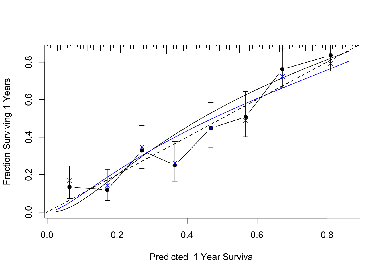
Validate predicted 1-year survival probabilities. Use a smooth `r ipacue()`
approach that does not require binning [@koo95haz] and use
less precise Kaplan-Meier estimates obtained by stratifying patients
by the predicted
probability, with at least 60 patients per group.
```{r cal, cap='Bootstrap validation of calibration curve. Dots represent apparent calibration accuracy; $\\times$ are bootstrap estimates corrected for overfitting, based on binning predicted survival probabilities and and computing Kaplan-Meier estimates. Black curve is the estimated observed relationship using `hare` and the blue curve is the overfitting-corrected `hare` estimate. The gray-scale line depicts the ideal relationship.',scap='Bootstrap validation of calibration curve for log-normal model'}
#| label: fig-psmcase-cal
set.seed(717)
cal <- calibrate(g, u=1, B=300)
plot(cal, subtitles=FALSE)
cal <- calibrate(g, cmethod='KM', u=1, m=60, B=300, pr=FALSE)
plot(cal, add=TRUE)
```
## Approximating the Full Model {#sec-psmcase-approx}
`r mrg(sound("psm-case-6"))`
The fitted log-normal model is perhaps too complex for routine use
and for routine data collection. Let us develop a simplified model
that can predict the predicted values of the full model with high
\index{accuracy!approximation}accuracy ($R^{2} = 0.96$). The
simplification is done using a fast
backward stepdown against the full model predicted values.
```{r }
Z <- predict(f)    # X*beta hat
a <- ols(Z ~ rcs(age,5)+sex+dzgroup+num.co+
             scoma+pol(adlsc,2)+race2+
             rcs(meanbp,5)+rcs(hrt,3)+rcs(resp,3)+
             temp+rcs(crea,4)+sod+rcs(wblc.i,3)+
             rcs(pafi.i,4), sigma=1, data=ac)
# sigma=1 is used to prevent sigma hat from being zero when
# R2=1.0 since we start out by approximating Z with all
#  component variables
fastbw(a, aics=10000)    # fast backward stepdown
```
```{r }
f.approx <- ols(Z ~ dzgroup + rcs(meanbp,5) + rcs(crea,4) + rcs(age,5) +
                rcs(hrt,3) + scoma + rcs(pafi.i,4) + pol(adlsc,2)+
                rcs(resp,3), x=TRUE, data=ac)
f.approx$stats
```
* Estimate variance-covariance matrix of the coefficients of reduced model `r ipacue()`
* This covariance matrix does not include the scale parameter
```{r }
V <- vcov(f, regcoef.only=TRUE)     # var(full model)
X <- cbind(Intercept=1, g$x)        # full model design
x <- cbind(Intercept=1, f.approx$x) # approx. model design
w <- solve(t(x) %*% x, t(x)) %*% X  # contrast matrix
v <- w %*% V %*% t(w)
```
Compare variance estimates (diagonals of `v`) with
variance estimates from a reduced model that is fitted against the
actual outcomes.
```{r }
f.sub <- psm(S ~ dzgroup + rcs(meanbp,5) + rcs(crea,4) + rcs(age,5) +
             rcs(hrt,3) + scoma + rcs(pafi.i,4) + pol(adlsc,2)+
             rcs(resp,3), dist='lognormal', data=ac)

r <- diag(v)/diag(vcov(f.sub,regcoef.only=TRUE))
r[c(which.min(r), which.max(r))]
```
`r ipacue()`
```{r}
f.approx$var <- v
anova(f.approx, test='Chisq', ss=FALSE)
```
Equation for simplified model:
```{r}
# Typeset mathematical form of approximate model
latex(f.approx)
```
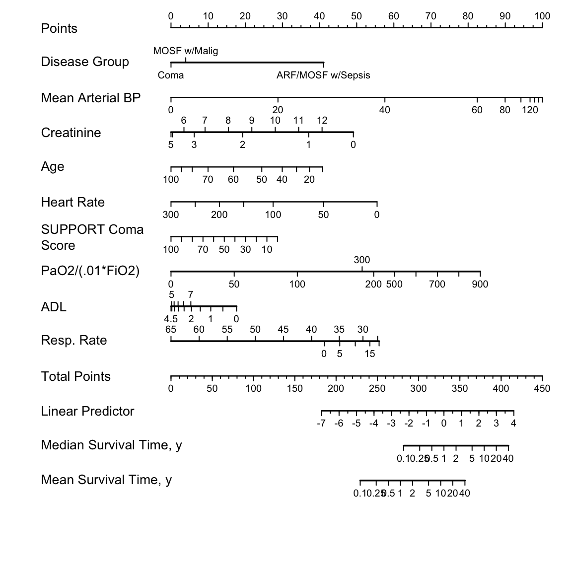
<br><br>
Nomogram for predicting median and mean survival time, based on
`r mrg(sound("psm-case-7"))` approximate model:
```{r}
# Derive R functions that express mean and quantiles
# of survival time for specific linear predictors
# analytically
expected.surv <- Mean(f)
quantile.surv <- Quantile(f)
expected.surv
quantile.surv
median.surv <- function(x) quantile.surv(lp=x)
```
```{r nomogram, h=6, w=6, cap='Nomogram for predicting median and mean survival time, based on approximation of full model',scap='Nomogram for simplified log-normal model'}
#| label: fig-psmcase-nomogram
spar(ps=10)
# Improve variable labels for the nomogram
f.approx <- Newlabels(f.approx, c('Disease Group','Mean Arterial BP',
          'Creatinine','Age','Heart Rate','SUPPORT Coma Score',
          'PaO2/(.01*FiO2)','ADL','Resp. Rate'))
nom <-
  nomogram(f.approx,
           pafi.i=c(0, 50, 100, 200, 300, 500, 600, 700, 800, 900),
           fun=list('Median Survival Time, y'=median.surv,
                    'Mean Survival Time, y'  =expected.surv),
           fun.at=c(.1,.25,.5,1,2,5,10,20,40))
plot(nom, cex.var=1, cex.axis=.75, lmgp=.25)
```
| Packages | Purpose | Functions |
|-----|-----|-----|
| `Hmisc` | Miscellaneous functions | `describe,ecdf,naclus,varclus,llist,spearman2,impute,latex` |
| `rms` | Modeling | `datadist,psm,rcs,ols,fastbw` |
| | Model presentation | `survplot,Newlabels,Function,Mean,Quantile,nomogram` |
| | Model validation | `validate,calibrate` |
: R packages and functions used. All packages are available on `CRAN`.
```{r echo=FALSE}
saveCap('19')
```