15  Regression Models for Continuous \(Y\) and Case Study in Ordinal Regression

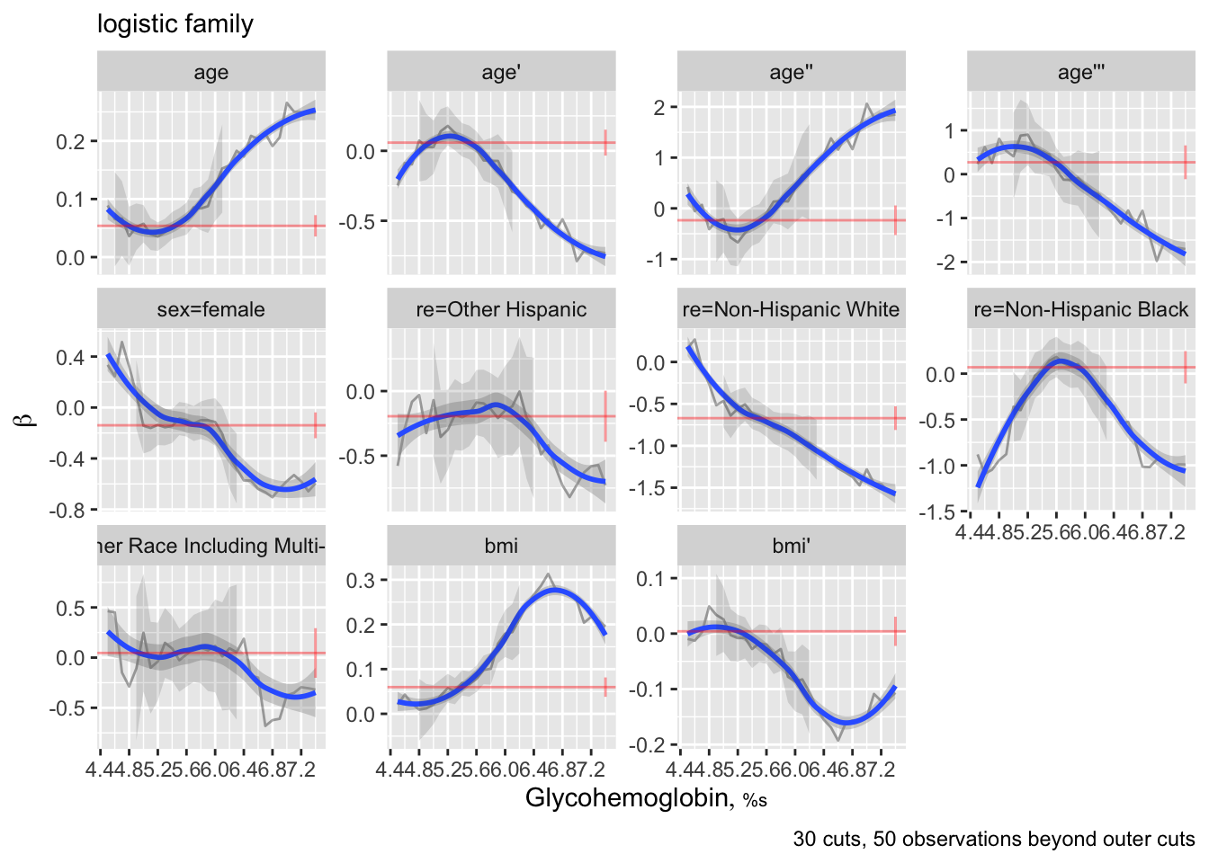
This chapter concerns univariate continuous \(Y\). There are many multivariable models for predicting such response variables.

A

• linear models with assumed normal residuals, fitted with ordinary least squares
• generalized linear models and other parametric models based on special distributions such as the gamma
• generalized additive models (GAMs)
• generalization of GAMs to also nonparametrically transform \(Y\)
• quantile regression (see Section Section 15.3)
• other robust regression models that, like quantile regression, use an objective different from minimizing the sum of squared errors (Venables & Ripley, 2003)
• semiparametric models based on the ranks of \(Y\), such as the Cox proportional hazards model and the proportional odds ordinal logistic model
• cumulative probability models (often called cumulative link models despite the fact that cumulative probabilities and not cumulative links are being computed) which are semiparametric models from a wider class of families than the logistic

Semiparametric models that treat \(Y\) as ordinal but not interval-scaled have many advantages including robustness and freedom of distributional assumptions for \(Y\) conditional on any given set of predictors. Advantages are demonstrated in a case study of a cumulative probability ordinal model. Some of the results are compared to quantile regression and OLS. Many of the methods used in the case study also apply to ordinary linear models.

B

15.1 Dataset and Descriptive Statistics

• Diabetes Mellitus (DM) type II (adult onset diabetes) is strongly associated with obesity
• Primary laboratory test for diabetes: glycosylated hemoglobin (\(\text{HbA}_{1c}\)), also called glycated hemoglobin, glycohemoglobin, or hemoglobin \(A_{1c}\).
• \(\text{HbA}_{1c}\) reflects average blood glucose for the preceding 60 to 90 days
• \(\text{HbA}_{1c}\) \(> 7.0\) usually taken as a positive diagnosis of diabetes
• Goal of analysis:
  • better understand effects of body size measurements on risk of DM
  • enhance screening for DM
• Best way to develop a model for DM screening is not to fit binary logistic model with \(\text{HbA}_{1c}\) > 7 as the response variable
  • All cutpoints are arbitrary; no justification for any putative cut
  • \(\text{HbA}_{1c}\) 2=6.9, 7.1=10
  • Larger standard errors of \(\hat{\beta}\), lower power, wider confidence bands
  • Better: predict continuous \(\text{HbA}_{1c}\) using continuous response model, then convert to probability \(\text{HbA}_{1c}\) exceeds any cutoff or estimate 0.9 quantile of \(\text{HbA}_{1c}\)
• Data: U.S. National Health and Nutrition Examination Survey (NHANES) from National Center for Health Statistics/CDC: www.cdc.gov/nchs/nhanes.htm (Centers for Disease Control and Prevention CDC. National Center for Health Statistics NCHS, 2010)
• age \(\geq 80\) coded as 80 by CDC
• Subset with age \(\geq 21\), neither diagnosed nor treated for DM
• Transform bmi, just for the spike histograms

CDE

require(rms)
options(prType='html')   # for print, summary, anova, describe
getHdata(nhgh)
w <- subset(nhgh, age >= 21 & dx==0 & tx==0, select=-c(dx,tx))
des <- describe(w, trans=list(bmi= list('log', log, exp)))
                                                                            
sparkline::sparkline(0)   # loads jQuery javascript for sparklines

maketabs(print(des, 'both'), wide=TRUE, initblank=TRUE)

Continuous

w Descriptives
15 Continous Variables of 18 Variables, 4629 Observations
Variable	Label	Units	n	Missing	Distinct	Info	Mean	pMedian	Gini |Δ|		Quantiles .05 .10 .25 .50 .75 .90 .95
seqn	Respondent sequence number		4629	0	4629	1.000	56902	56902	3501		52136 52633 54284 56930 59495 61079 61641
age	Age	years	4629	0	703	1.000	48.57	48.29	19.85		23.33 26.08 33.92 46.83 61.83 74.83 80.00
wt	Weight	kg	4629	0	890	1.000	80.49	78.9	22.34		52.44 57.18 66.10 77.70 91.40 106.52 118.00
ht	Standing Height	cm	4629	0	512	1.000	167.5	167.4	11.71		151.1 154.4 160.1 167.2 175.0 181.0 184.8
bmi	Body Mass Index	kg/m2	4629	0	1994	1.000	28.59	28.02	6.965		20.02 21.35 24.12 27.60 31.88 36.75 40.68
leg	Upper Leg Length	cm	4474	155	216	1.000	38.39	38.4	4.301		32.0 33.5 36.0 38.4 41.0 43.3 44.6
arml	Upper Arm Length	cm	4502	127	156	1.000	37.01	37	3.116		32.6 33.5 35.0 37.0 39.0 40.6 41.7
armc	Arm Circumference	cm	4499	130	290	1.000	32.87	32.65	5.475		25.4 26.9 29.5 32.5 35.8 39.1 41.4
waist	Waist Circumference	cm	4465	164	716	1.000	97.62	96.9	17.18		74.8 78.6 86.9 96.3 107.0 117.8 125.0
tri	Triceps Skinfold	mm	4295	334	342	1.000	18.94	18.7	9.463		7.2 8.8 12.0 18.0 25.2 31.0 33.8
sub	Subscapular Skinfold	mm	3974	655	329	1.000	20.8	20.6	9.124		8.60 10.30 14.40 20.30 26.58 32.00 35.00
gh	Glycohemoglobin	%	4629	0	63	0.994	5.533	5.5	0.5411		4.8 5.0 5.2 5.5 5.8 6.0 6.3
albumin	Albumin	g/dL	4576	53	26	0.990	4.261	4.25	0.3528		3.7 3.9 4.1 4.3 4.5 4.7 4.8
bun	Blood urea nitrogen	mg/dL	4576	53	50	0.995	13.03	12.5	5.309		7 8 10 12 15 19 22
SCr	Creatinine	mg/dL	4576	53	167	1.000	0.8887	0.855	0.2697		0.58 0.62 0.72 0.84 0.99 1.14 1.25

Categorical

w Descriptives
3 Categorical Variables of 18 Variables, 4629 Observations
Variable	Label	n	Missing	Distinct
sex		4629	0	2
re	Race/Ethnicity	4629	0	5
income	Family Income	4389	240	14

dd <- datadist(w); options(datadist='dd')

15.2 The Linear Model

The most popular multivariable model for analyzing a univariate continuous \(Y\) is the the linear model \[ E(Y | X) = X \beta, \] where \(\beta\) is estimated using ordinary least squares, that is, by solving for \(\hat{\beta}\) to minimize \(\sum (Y_{i} - X \hat{\beta})^{2}\).

• To compute \(P\)-values and confidence limits using parametric methods (and for least squares estimates to coincide with maximum likelihood estimates) we would have to assume that \(Y | X\) is normal with mean \(X \beta\) and constant variance \(\sigma^2\) ¹

F

¹ The latter assumption may be dispensed with if we use a robust Huber-White or bootstrap covariance matrix estimate. Normality may sometimes be dispensed with by using bootstrap confidence intervals, but this would not fix inefficiency problems with OLS when residuals are non-normal.

15.2.1 Checking Assumptions of OLS and Other Models

• First see if gh would make a Gaussian residuals model fit
• Use ordinary regression on 4 key variables to collapse into one variable (predicted mean from OLS model)
• Stratify predicted mean into 6 quantile groups
• Apply the normal inverse ECDF of gh to these strata and check for normality and constant \(\sigma^2\)
• ECDF is for \(\Pr[Y \leq y | X]\) but for ordinal modeling we want to state models in terms of \(\Pr[Y \ge y | X]\) so take 1 - ECDF before inverse transforming

G

f <- ols(gh ~ rcs(age,5) + sex + re + rcs(bmi, 3), data=w)
setDT(w)    # make w a data.table
w[, pgh  := fitted(f)]
w[, pgh6 := cut2(pgh, g=6)]
u <- w[, ecdfSteps(gh, extend=FALSE), by=pgh6]    # ecdfSteps is in Hmisc
v <- rbind(data.table(trans='paste(Phi^-1, (F[n](x)))', u[, z := qnorm(1 - y)     ]),
           data.table(trans='logit(F[n](x))',           u[, z := qlogis(1 - y)    ]),
           data.table(trans='-log(-log(F[n](x)))',      u[, z := -log(-log(1 - y))]),
           data.table(trans='log(-log(1-F[n](x)))',     u[, z := log(-log(y))     ]))
v <- v[! is.infinite(z)]
ggplot(v, aes(x, z, color=pgh6)) + geom_step() + 
  facet_wrap(~ trans, label='label_parsed', scales='free_y') +
  xlab(expression(HbA[`1c`])) + theme(legend.position='bottom')

# Get slopes of pgh for some cutoffs of Y
# Use glm complementary log-log link on Prob(Y < cutoff) to
# get log-log link on Prob(Y >= cutoff)
r <- NULL
for(link in c('logit','probit','cloglog'))
  for(k in c(5, 5.5, 6)) {
    co <- coef(glm(gh < k ~ pgh, data=w, family=binomial(link)))
    r <- rbind(r, data.frame(link=link, cutoff=k,
                             slope=round(co[2],2)))
}
print(r, row.names=FALSE)

    link cutoff slope
   logit    5.0 -3.39
   logit    5.5 -4.33
   logit    6.0 -5.62
  probit    5.0 -1.69
  probit    5.5 -2.61
  probit    6.0 -3.07
 cloglog    5.0 -3.18
 cloglog    5.5 -2.97
 cloglog    6.0 -2.51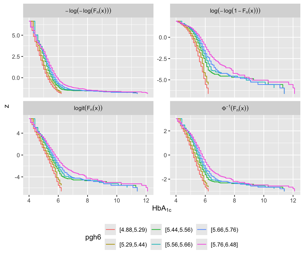

Figure 15.1: Examination of normality and constant variance assumption, and assumptions for various ordinal models

• Lower right curves are not linear, implying that a normal conditional distribution cannot work for gh²
• There is non-parallelism for the logit model
• Other graphs will be used to guide selection of an ordinal model below

H

² They are not parallel either.

The rms ordParallel function makes it easy to vary coefficients over a continuum of cutoffs, and it has a algorithm for choosing cutpoints given a specify maximum number of cutoffs. As this allows different predictors to have different amounts of non-parallelism, this may be preferred to the 6-tiles approach.

f <- orm(gh ~ rcs(age,5) + sex + re + rcs(bmi, 3), data=w, x=TRUE, y=TRUE)
ordParallel(f)

When there are multiple terms, it is difficult to interpret this plot. There is an option to combine all the terms for each predictor into a single partial linear predictor. Then y-varying effects are assessed with respect to this predictor summary measure. By default these partial linear predictors are scaled by their inter-quartile-range over observations so that weak predictors will not have exaggerated/irrelevant y-cutoff-dependencies.

ordParallel(f, terms=TRUE)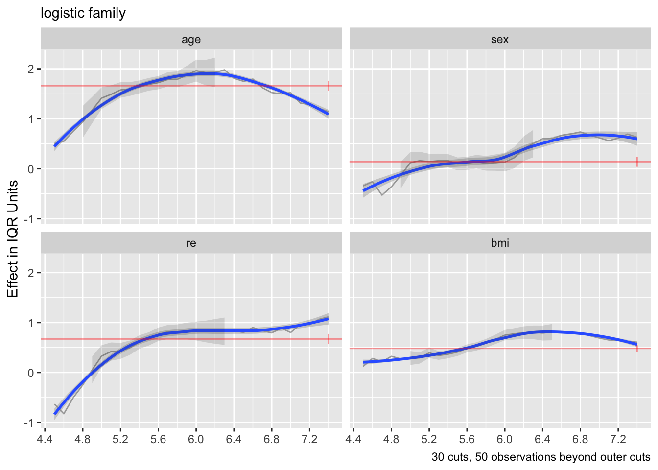

The above two plots were for the logit link. Re-run using the log-log link.

f <- orm(gh ~ rcs(age,5) + sex + re + rcs(bmi, 3), family='loglog',
         data=w, x=TRUE, y=TRUE)
ordParallel(f, terms=TRUE)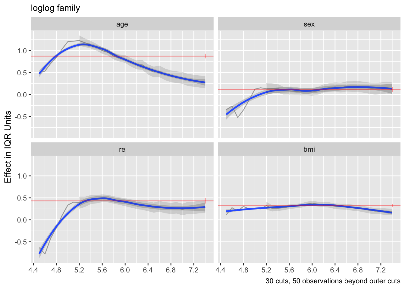

Effects appear to be more constant.

ordParallel has an onlydata option to make it produce a data frame instead of a graphic. The data frame is a stacked version of all the one-number “terms” summaries. The number of observations in the stacked data frame will be the number of cuts multiplied by the number of observations. A variable obs is included in the data frame so that one can see which original observation numbers correspond to each row of the stacked data. obs can be used as the cluster argument to rms::robcov to get robust cluster sandwich variance-covariance matrix estimates. These can be used to get wald tests for interactions between cutoffs and covariate, i.e., tests of parallelism. The following example shows how to do this for the two link functions.

testpar <- function(form, link) {
  f  <- orm(form, data=w, family=link, x=TRUE, y=TRUE)
  do <- ordParallel(f, onlydata=TRUE, maxcuts=30)
  g  <- orm(Yge_cut ~ (age + sex + bmi + re) * Ycut, data=do, x=TRUE, y=TRUE)
  h  <- robcov(g, do$obs)
  print(anova(h))
  invisible()
}
form <- gh ~ rcs(age,5) + sex + re + rcs(bmi, 3)
testpar(form, 'logistic')    # Chunk test for global parallelism 151.17
testpar(form, 'loglog')      # Chunk test 140.8

Another approach to goodness of fit is internal calibration plots. For a series of gh cutoffs plot the estimated actual probability of exceeding the cutoff as a function of the predicted probability of exceeding it.

gcuts <- c(5.5, 6, 6.5, 7)
intCalibration(f, ycuts=gcuts) + labs(subtitle=f$family)

Calibration-in-the-large:

   y Mean Predicted P(Y > y) Observed P(Y > y)
 5.5                 0.41770           0.42623
 6.0                 0.09299           0.09419
 6.5                 0.02870           0.02636
 7.0                 0.01650           0.01339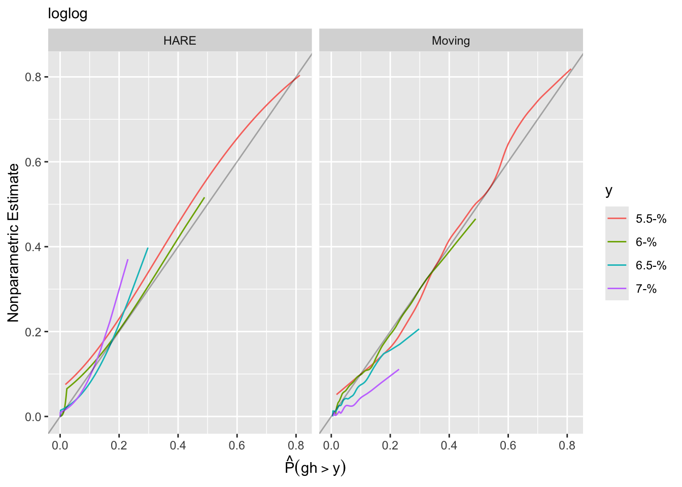

g <- update(f, family='logistic')
intCalibration(g, ycuts=gcuts) + labs(subtitle=g$family)

Calibration-in-the-large:

   y Mean Predicted P(Y > y) Observed P(Y > y)
 5.5                 0.43578           0.42623
 6.0                 0.09590           0.09419
 6.5                 0.02646           0.02636
 7.0                 0.01338           0.01339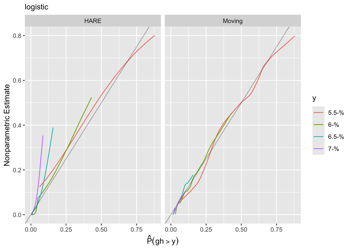

Using the adaptive linear spline HARE estimates, the logit link fits less well.

A different calibration plan is made by plotting both predicted and observed exceedance probabilities against a covariate.

intCalibration(f, ycuts=gcuts, x=w$age) + labs(subtitle=f$famiy)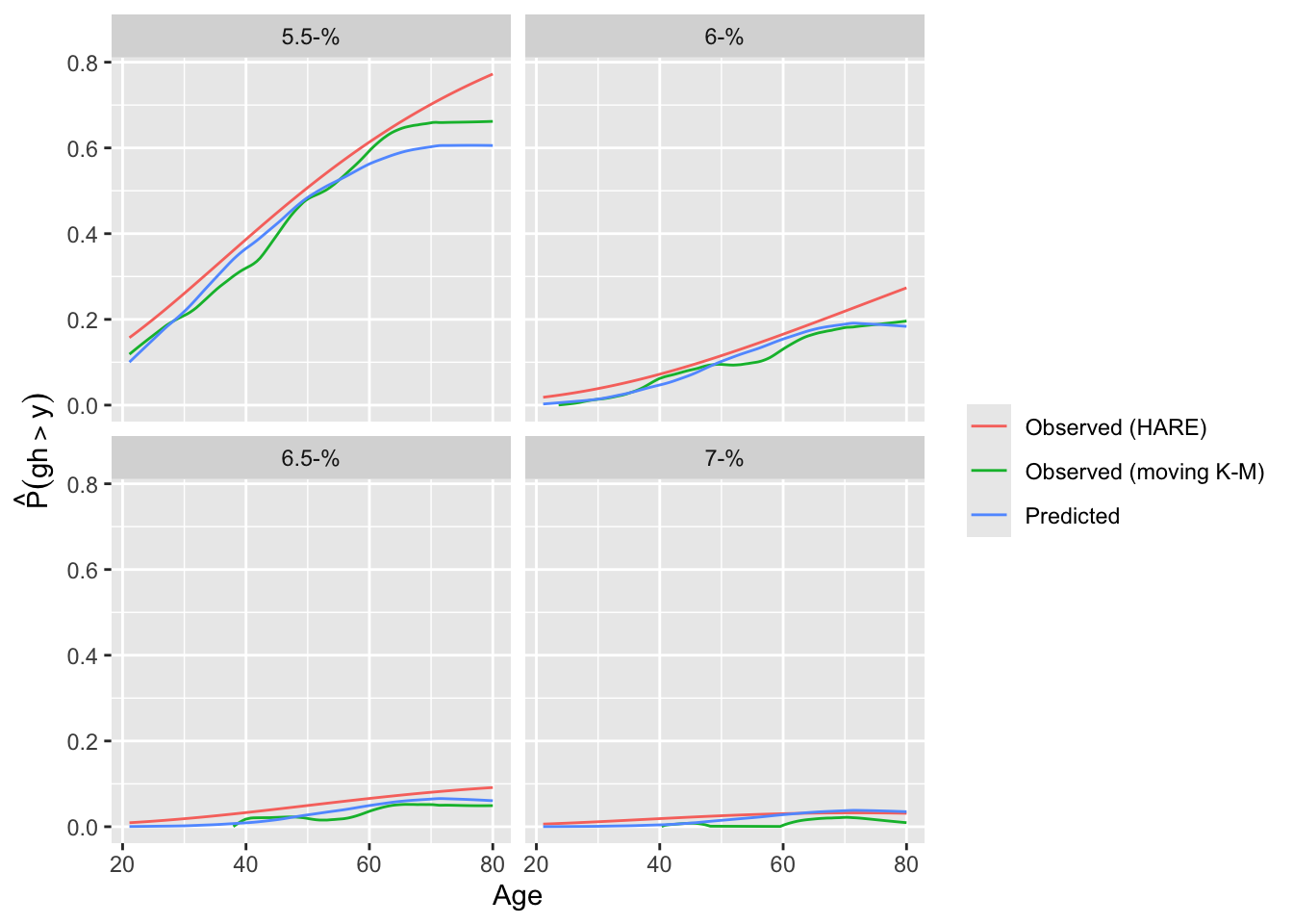

intCalibration(g, ycuts=gcuts, x=w$age) + labs(subtitle=g$famiy)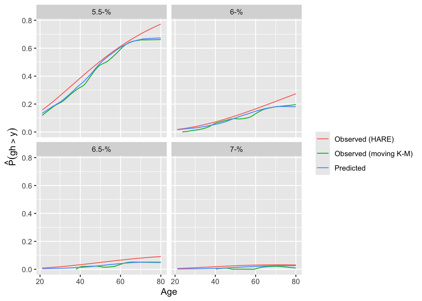

Finally, the rms Olinks function computes deviance measures for a series of link functions. Though this may not detect Y-dependency of effects (nonparallelism) with respect to a single predictor, it is useful for choosing the overall model. Model fits are automatically re-run by Olinks for a series of links not used in the current fit.

Olinks(f)

      link null.deviance deviance      AIC       LR    R2
1   loglog      26909.83 25580.57 25726.57 1329.262 0.249
2 logistic      26909.83 25522.82 25668.82 1387.005 0.258
3   probit      26909.83 25621.47 25767.47 1288.363 0.242
4  cloglog      26909.83 26096.27 26242.27  813.562 0.160

Oddly, the logit link had the smallest deviance. More study of comparing deviances is needed.

15.3 Quantile Regression

• Ruled out OLS and semiparametric proportional odds model
• Quantile regression (Koenker, 2005; Koenker & Bassett, 1978) is a different approach to modeling \(Y\)
• No distributional assumptions other than continuity of \(Y\)
• All the usual right hand side assumptions
• When there is a single predictor that is categorical, quantile regression coincides with ordinary sample quantiles stratified by that predictor
• Is transformation invariant - pre-transforming \(Y\) not important

I

Let \(\rho_{\tau}(y) = y(\tau - [y < 0])\). The \(\tau^{\mathrm th}\) sample quantile is the minimizer \(q\) of \(\sum_{i-1}^{n}\rho_{\tau}(y_{i}-q)\). For a conditional \(\tau^{\mathrm th}\) quantile of \(Y | X\) the corresponding quantile regression estimator \(\hat{\beta}_{\tau}\) minimizes \(\sum_{i=1}^{n}\rho_{\tau}(Y_{i}-X\beta)\). Quantile regression is not as efficient at estimating quantiles as is ordinary least squares at estimating the mean, if the latter’s assumptions hold. Koenker’s quantreg package in R (Koenker, 2009) implements quantile regression, and the rms package’s Rq function provides a front-end that gives rise to various graphics and inference tools. If we model the median gh as a function of covariates, only the \(X\beta\) structure need be correct. Other quantiles (e.g., \(90^\text{th}\) percentile) can be directly modeled but standard errors will be much larger as it is more difficult to precisely estimate outer quantiles.

J

15.4 Ordinal Regression Models for Continuous \(Y\)

• Advantages of semiparametric models (e.g., quantile regression and cumulative probability ordinal models
• For ordinal cumulative probability models, there is no distributional assumption for \(Y\) given a setting of \(X\)
• Assume only a connection between distributions of \(Y\) for different \(X\)
• Applying an increasing 1–1 transformation to \(Y\) results in no change to regression coefficient estimates³
• Regression coefficient estimates are completely robust to extreme \(Y\) values⁴
• Estimates of quantiles of \(Y\) are exactly transformation-preserving, e.g., estimate of median of \(\log Y\) is exactly the log of the estimate of median \(Y\)
• Manuguerra & Heller (2010) developed an ordinal model for continuous \(Y\) which they incorrectly labeled semi-parametric and is actually a lower-dimensional flexible parametric model that instead of having intercepts has a spline function of \(y\).

K

³ For symmetric distributions applying a decreasing transformation will negate the coefficients. For asymmetric distributions (e.g., Gumbel), reversing the order of \(Y\) will do more than change signs.

⁴ Only an estimate of mean \(Y\) from these \(\hat{\beta}\)s is non-robust.

---

For a general continuous distribution function \(F(y)\), an ordinal regression model based on cumulative probabilities may be stated as follows⁵. Let the ordered unique values of \(Y\) be denoted by \(y_{1}, y_{2}, \dots, y_{k}\) and let the intercepts associated with \(y_{1}, \dots, y_{k}\) be \(\alpha_{1}, \alpha_{2}, \dots, \alpha_{k}\), where \(\alpha_{1} = \infty\) because \(\Pr[Y \geq y_{1}] = 1\). Let \(\alpha_{y} = \alpha_{i}, i:y_{i}=y\). Then \[ \Pr[Y \geq y_{i} | X] = F(\alpha_{i} + X\beta) = F(\alpha_{y_{i}} + X\beta) \] For the OLS fully parametric case, the model may be restated

L

⁵ It is more traditional to state the model in terms of \(\Pr[Y \leq y | X]\) but we use \(\Pr[Y \geq y | X]\) so that higher predicted values are associated with higher \(Y\).

\[\begin{array}{c} \Pr[Y \geq y | X] = \Pr[\frac{Y-X\beta}{\sigma} \geq \frac{y-X\beta}{\sigma}]\\ = 1-\Phi(\frac{y-X\beta}{\sigma}) = \Phi(\frac{-y}{\sigma}+\frac{X\beta}{\sigma}) \end{array}\]

so that to within an additive constant ⁶ \(\alpha_{y} = \frac{-y}{\sigma}\) (intercepts \(\alpha\) are linear in \(y\) whereas they are arbitrarily descending in the ordinal model), and \(\sigma\) is absorbed in \(\beta\) to put the OLS model into the new notation. The general ordinal regression model assumes that for fixed \(X_{1}, X_{2}\),

⁶ \(\hat{\alpha_{y}}\) are unchanged if a constant is added to all \(y\).

\[\begin{array}{c} F^{-1}(\Pr[Y \geq y | X_{2}]) - F^{-1}(\Pr[Y \geq y | X_{1}])\\ = (X_{2} - X_{1})\beta \end{array}\]

independent of the \(\alpha\)s (parallelism assumption). If \(F = [1 + \exp(-y)]^{-1}\), this is the proportional odds assumption.

Common choices of \(F\), implemented in the rms orm function, are shown in Table Table 15.1.

M

Table 15.1: Distribution families used in ordinal cumulative probability models. \(\Phi\) denotes the Gaussian cumulative distribution function. For the Connection column, \(P_{1}=\Pr[Y \geq y | X_{1}], P_{2}=\Pr[Y \geq y | X_{2}], \Delta=(X_{2}-X_{1})\beta\). The connection specifies the only distributional assumption if the model is fitted semiparametrically, i.e, contains an intercept for every unique \(Y\) value less one. For parametric models, \(P_{1}\) must be specified absolutely instead of just requiring a relationship between \(P_{1}\) and \(P_{2}\). For example, the traditional Gaussian parametric model specifies that \(\Pr[Y \geq y | X] = 1 - \Phi(\frac{y - X\beta}{\sigma}) = \Phi(\frac{-y + X\beta}{\sigma})\).

Distribution	\(F\)	Inverse (Link Function)	Link Name	Connection
Logistic	\([1 + \exp(-y)]^{-1}\)	\(\log(\frac{y}{1-y})\)	logit	\(\frac{P_{2}}{1-P_{2}} = \frac{P_{1}}{1-P_{1}} \exp(\Delta)\)
Gaussian	\(\Phi(y)\)	\(\Phi^{-1}(y)\)	probit	\(P_{2}=\Phi(\Phi^{-1}(P_{1})+\Delta)\)
Gumbel maximum value	\(\exp(-\exp(-y))\)	\(\log(-\log(y))\)	\(\log-\log\)	\(P_{2}=P_{1}^{\exp(\Delta)}\)
Gumbel minimum value	\(1 - \exp(-\exp(y))\)	\(\log(-\log(1 - y))\)	complementary \(\log-\log\)	\(1-P_{2}=(1-P_{1})^{\exp(\Delta)}\)
Cauchy	\(\frac{1}{\pi}\tan^{-1}(y) + \frac{1}{2}\)	\(\tan[\pi(y - \frac{1}{2})]\)	cauchit

The Gumbel maximum value distribution is also called the extreme value type I distribution. This distribution (\(\log-\log\) link) also represents a continuous time proportional hazards model. The hazard ratio when \(X\) changes from \(X_{1}\) to \(X_{2}\) is \(\exp(-(X_{2} - X_{1}) \beta)\). The mean of \(Y | X\) is easily estimated by computing \[ \sum_{i=1}^{k} y_{i} \hat{\Pr}[Y = y_{i} | X] \] and the \(q^\text{th}\) quantile of \(Y | X\) is \(y\) such that
\(F^{-1}(1 - q) - X\hat{\beta} = \hat{\alpha}_{y}\).⁷ The orm function in the rms package takes advantage of the information matrix being of a sparse tri-band diagonal form for the intercept parameters. This makes the computations efficient even for hundreds of intercepts (i.e., unique values of \(Y\)). orm is made to handle continuous \(Y\). Ordinal regression has nice properties in addition to those listed above, allowing for

N

⁷ The intercepts have to be shifted to the left one position in solving this equation because the quantile is such that \(\Pr[Y \leq y] = q\) whereas the model is stated in terms of \(\Pr[Y \geq y]\).

• estimation of quantiles as efficiently as quantile regression if the parallel slopes assumptions hold
• efficient estimation of mean \(Y\)
• direct estimation of \(\Pr[Y\geq y | X]\)
• arbitrary clumping of values of \(Y\), while still estimating \(\beta\) and mean \(Y\) efficiently⁸
• solutions for \(\hat{\beta}\) using ordinary Newton-Raphson or other popular optimization techniques
• being based on a standard likelihood function, penalized estimation can be straightforward
• Wald, score, and likelihood ratio \(\chi^2\) tests that are more powerful than tests from quantile regression

O

⁸ But it is not sensible to estimate quantiles of \(Y\) when there are heavy ties in \(Y\) in the area containing the quantile.

To summarize how assumptions of parametric models compare to assumptions of semiparametric models, consider the ordinary linear model or its special case the equal variance two-sample \(t\)-test, vs. the probit or logit (proportional odds) ordinal model or their special cases the Van der Waerden (normal-scores) two-sample test or the Wilcoxon test. All the assumptions of the linear model other than independence of residuals are captured in the following (written in traditional \(Y\leq y\) form):

P

\[\begin{array}{c} F(y|X) = \Pr[Y \leq y|X] = \Phi(\frac{y-X\beta}{\sigma})\\ \Phi^{-1}(F(y|X)) = \frac{y-X\beta}{\sigma} \end{array}\]

spar(mfrow=c(1,2), left=2)
pinv <- expression(paste(Phi^{-1},  '(F(y', '|', 'X))'))
plot(0, 0, xlim=c(0, 1), ylim=c(-2, 2), type='n', axes=FALSE,
     xlab=expression(y), ylab='')
mtext(pinv, side=2, line=1)
axis(1, labels=FALSE, lwd.ticks=0)
axis(2, labels=FALSE, lwd.ticks=0)
abline(a=-1.5, b=1)
abline(a=0, b=1)
arrows(.5, -1.5+.5, .5, 0+.5, code=3, length=.1)
text(.525, .5*(-1.5+.5+.5), expression(-Delta*X*beta/sigma), adj=0)
g <- function(x) -2.2606955+11.125231*x-37.772783*x^2+56.776436*x^3-
  26.861103*x^4
x <- seq(0, .9, length=150)
pinv <- expression(atop(paste(Phi^{-1},  '(F(y', '|', 'X))'),
    paste(logit, '(F(y', '|', 'X))')))
plot(0, 0, xlim=c(0, 1), ylim=c(-2, 2), type='n', axes=FALSE,
     xlab=expression(y), ylab='')
mtext(pinv, side=2, line=1)
axis(1, labels=FALSE, lwd.ticks=FALSE)
axis(2, labels=FALSE, lwd.ticks=FALSE)
lines(x, g(x))
lines(x, g(x)+1.5)
arrows(.5, g(.5), .5, g(.5)+1.5, code=3, length=.1)
text(.525, .5*(g(.55) + g(.55)+1.5), expression(-Delta*X*beta), adj=0)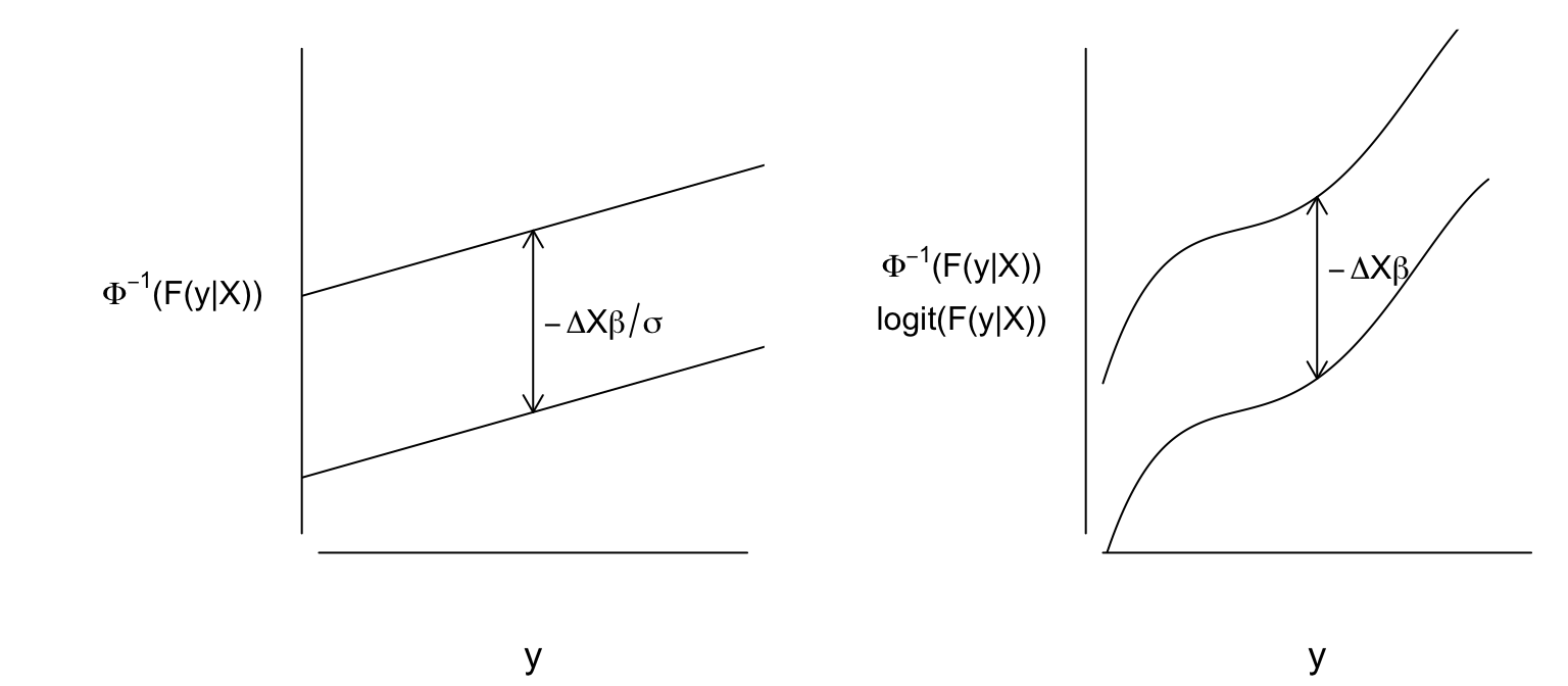

Figure 15.2: Assumptions of the linear model (left panel) and semiparametric ordinal probit or logit (proportional odds) models (right panel). Ordinal models do not assume any shape for the distribution of \(Y\) for a given \(X\); they only assume parallelism.

On the other hand, ordinal models assume the following: \[ \Pr[Y \leq y|X] = F(g(y)-X\beta), \] where \(g\) is unknown and may be discontinuous. From this point we revert back to \(Y\geq y\) notation so that \(Y\) increases as \(X\beta\) increases.

Global Modeling Implications

• Ordinal regression invariant to choice of transformation of \(Y\)
• \(Y\) needs to be ordinal
• Difference in two ordinal variables is not necessarily ordinal
• \(\rightarrow\) Never analyze differences in regression
• \(Y\)=final value, adjust for baseline values as covariates

Q

15.5 Ordinal Regression Applied to \(\text{HbA}_{1c}\)

• In Figure 15.1, logit inverse curves are not parallel so proportional odds assumption does not hold
• log-log link yields highest degree of parallelism and most constant regression coefficients across cutoffs of gh so use this link in an ordinal regression model (linearity of the curves is not required)

R

15.5.1 Checking Fit for Various Models Using Age

S

Another way to examine model fit is to flexibly fit the single most important predictor (age) using a variety of methods, and comparing predictions to sample quantiles and means based on overlapping subsets on age, each subset being subjects having age \(< 5\) years away from the point being predicted by the models. Here we predict the 0.5, 0.75, and 0.9 quantiles and the mean. For quantiles we can compare to quantile regression(discussed below) and for means we compare to OLS.

require(data.table)
require(ggplot2)
estimands  <- .q(q2, q3, p90, mean)
links      <- .q(logistic, probit, loglog, cloglog)
estimators <- c(.q(empirical, ols, QR), links)
ages       <- 25 : 75
nage       <- length(ages)
yhat       <- numeric(length(ages))
fmt <- function(x) format(round(x, 3), nsmall=3)

r   <- expand.grid(estimand=estimands, estimator=estimators, age=ages, 
                   y=NA_real_, stringsAsFactors=FALSE)
setDT(r)
# Discard irrelevant methods for estimands
r   <- r[! (estimand == 'mean' & estimator == 'QR') &
         ! (estimand %in% .q(q2, q3, p90) & estimator == 'ols'), ]
# Find all used combinations
rc  <- r[age == 25]
rc[, age := NULL]

mod  <- gh ~ rcs(age,6)

# Compute estimates for all relevant combinations of estimands & estimators

for(eor in rc[, unique(estimator)]) {
  if(eor == 'empirical') {
    emp <- matrix(NA, nrow=nage, ncol=4,
                  dimnames=list(NULL, .q(mean, q2, q3, p90)))
    for(j in 1 : length(ages)) {
    s <- which(abs(w$age - ages[j]) < 5)
    y <- w$gh[s]
    a <- quantile(y, probs=c(0.5, 0.75, 0.90))
    emp[j, ] <- c(mean(y), a)
    }
  }
  else if(eor == 'ols')   fit <- ols(mod, data=w)
  else if(eor %in% links) fit <- orm(mod, data=w, family=eor)
  
  for(eand in rc[estimator == eor, unique(estimand)]) {
    qa <- switch(eand, q2=0.5, q3=0.75, p90=0.90)
    yhat <- if(eor == 'ols') Predict(fit, age=ages, conf.int=FALSE)$yhat
    else if(eor == 'empirical') emp[, eand] 
    else if(eor == 'QR') {
      fit <- Rq(mod, data=w, tau=qa)
      Predict(fit, age=ages, conf.int=FALSE)$yhat
      }
    else {
      fun <- switch(eand,
                    mean = Mean(fit),
                    Quantile(fit))
      fu <- if(eand == 'mean') fun
      else function(x) fun(qa, x) 
      Predict(fit, age=ages, fun=fu, conf.int=FALSE)$yhat
    }
   r[estimand == eand & estimator == eor, y := yhat]
  }
}

# Compute age-specific differences between estimates and empirical
# estimates, then compute mean absolute differences across all ages

dif <- r[estimator != 'empirical']

for(eor in rc[, setdiff(unique(estimator), 'empirical')]) 
  for(eand in rc[estimator == eor, unique(estimand)])
    dif[estimator == eor         & estimand == eand]$y <-
      r[estimator == eor         & estimand == eand]$y -
      r[estimator == 'empirical' & estimand == eand]$y
mad  <- dif[, .(ad = mean(abs(y))), by=.(estimand, estimator)] 
mad2 <- mad[, .(value = paste(fmt(ad), collapse='\n'),
                label = paste(estimator, collapse='\n'),
                x     = if(estimand == 'p90') 60  else 25,
                y     = if(estimand == 'p90') 5.5 else 6.2),
            by=.(estimand)]

ggplot() + geom_line(aes(x=age, y=y, col=estimator),
                     data=r[estimator != 'empirical']) + 
  geom_point(aes(x=age, y=y, alpha=I(0.35)),
             data=r[estimator == 'empirical']) +
  facet_wrap(~ estimand) +
  geom_text(aes(x=x,    y=y, label=label, hjust='left', size=I(3)), data=mad2) +
  geom_text(aes(x=x+10, y=y, label=value, hjust='left', size=I(3)), data=mad2) +
  guides(color=guide_legend(title='')) +
  theme(legend.position='bottom')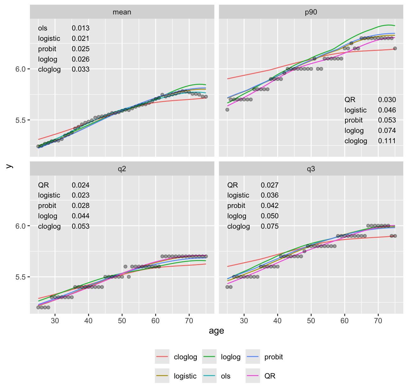

Figure 15.3: Three estimated quantiles and estimated mean using 6 methods, compared against caliper-matched sample quantiles/means (circles). Numbers are mean absolute differences between predicted and sample quantities using overlapping intervals of age and caliper matching. QR:quantile regression.

T

It can be seen in Figure 15.3 that models dedicated to a specific task (quantile regression for quantiles and OLS for means) were best for those tasks. Although the log-log ordinal cumulative probability model did not estimate the median as accurately as some other methods, it does well for the 0.75 and 0.9 quantiles and is the best compromise overall because of its ability to also directly predict the mean as well as quantities such as \(\Pr[\text{HbA}_{1c} > 7 | X]\). For here on we focus on the log-log ordinal model. Going back to the bottom left of Figure 15.1, let’s look at quantile groups of predicted \(\text{HbA}_{1c}\) by OLS and plot predicted distributions of actual \(\text{HbA}_{1c}\) against empirical distributions.

U

###w$pghg <- cut2(pgh, g=6)
f  <- orm(gh ~ pgh6, family='loglog', data=w)
lp <- predict(f, newdata=data.frame(pgh6=levels(w$pgh6)))
ep <- ExProb(f)  # Exceedance prob. functn. generator in rms
z  <- ep(lp)
j  <- order(w$pgh6)  # puts in order of lp (levels of pghg)
plot(z, xlim=c(4, 7.5), data=w[j,c('pgh6', 'gh')])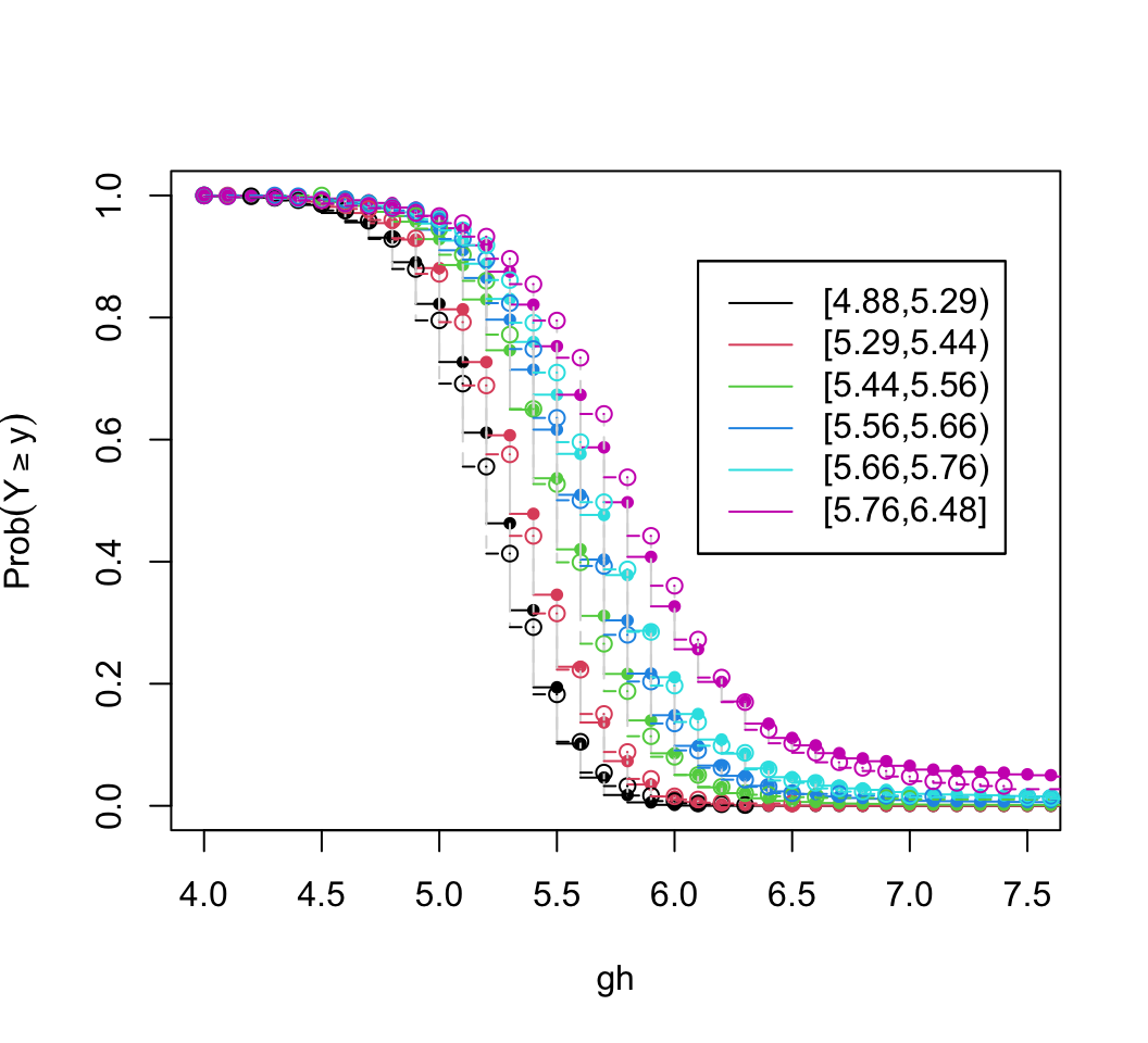 

Figure 15.4: Observed (dashed lines, open circles) and predicted (solid lines, closed circles) exceedance probability distributions from a model using 6-tiles of OLS-predicted \(\text{HbA}_{1c}\). Key shows quantile group intervals of predicted mean \(\text{HbA}_{1c}\).

Agreement between predicted and observed exceedance probability distributions is excellent in Figure 15.4. To return to the initial look at a linear model with assumed Gaussian residuals, fit a probit ordinal model and compare the estimated intercepts to the linear relationship with gh that is assumed by the normal distribution.

V

spar(bty='l')
f <- orm(gh ~ rcs(age,6), family='probit', data=w)
g <- ols(gh ~ rcs(age,6), data=w)
s <- g$stats['Sigma']
yu <- f$yunique[-1]
r <- quantile(w$gh, c(.005, .995))
alphas <- coef(f)[1:num.intercepts(f)]
plot(-yu / s, alphas, type='l', xlim=rev(- r / s), 
     xlab=expression(-y/hat(sigma)), ylab=expression(alpha[y]))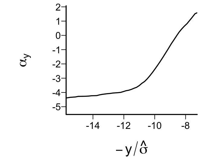

Figure 15.5: Estimated intercepts from probit model

Figure 15.5 depicts a significant departure from that implied by Gaussian residuals.

15.5.2 Examination of BMI

Using the log-log model, we first check the adequacy of BMI as a summary of height and weight for estimating median gh.

• Adjust for age (without assuming linearity) in every case
• Look at ratio of coefficients of log height and log weight
• Use AIC to judge whether BMI is an adequate summary of height and weight

W

f <- orm(gh ~ rcs(age,5) + log(ht) + log(wt),
         family='loglog', data=w)
f

-log-log Ordinal Regression Model

orm(formula = gh ~ rcs(age, 5) + log(ht) + log(wt), data = w, 
    family = "loglog")

	Model Likelihood Ratio Test	Discrimination Indexes	Rank Discrim. Indexes
Obs 4629	LR χ2 1126.94	R2 0.217	ρ 0.486
ESS 4602.2	d.f. 6	R26,4629 0.215	Dxy 0.359
Distinct Y 63	Pr(>χ2) <0.0001	R26,4602.2 0.216
Y0.5 5.5	Score χ2 1262.81	|Pr(Y ≥ median)-½| 0.153
max |∂log L/∂β| 2×10-10	Pr(>χ2) <0.0001

	β	S.E.	Wald Z	Pr(>|Z|)
age	0.0398	0.0055	7.29	<0.0001
age'	-0.0158	0.0275	-0.57	0.5657
age''	-0.0072	0.0866	-0.08	0.9333
age'''	0.0309	0.1135	0.27	0.7853
ht	-3.0680	0.2789	-11.00	<0.0001
wt	1.2748	0.0704	18.10	<0.0001

aic <- NULL
for(mod in list(gh ~ rcs(age,5) + rcs(log(bmi),5),
                gh ~ rcs(age,5) + rcs(log(ht),5) + rcs(log(wt),5),
                gh ~ rcs(age,5) + rcs(log(ht),4) * rcs(log(wt),4)))
  aic <- c(aic, AIC(orm(mod, family='loglog', data=w)))
print(aic)

[1] 25910.77 25910.17 25906.03

The ratio of the coefficient of log height to the coefficient of log weight is -2.4, which is between what BMI uses and the more dimensionally reasonable weight / height\(^{3}\). By AIC, a spline interaction surface between height and weight does slightly better than BMI in predicting \(\text{HbA}_{1c}\), but a nonlinear function of BMI is barely worse. It will require other body size measures to displace BMI as a predictor. As an aside, compare this model fit to that from the Cox proportional hazards model. The Cox model uses a conditioning argument to obtain a partial likelihood free of the intercepts \(\alpha\) (and requires a second step to estimate these log discrete hazard components) whereas we are using a full marginal likelihood of the ranks of \(Y\) (Kalbfleisch & Prentice, 1973).

X

cph(Surv(gh) ~ rcs(age,5) + log(ht) + log(wt), data=w)

Cox Proportional Hazards Model

cph(formula = Surv(gh) ~ rcs(age, 5) + log(ht) + log(wt), data = w)

	Model Tests	Discrimination Indexes
Obs 4629	LR χ2 1120.20	R2 0.215
Events 4629	d.f. 6	R26,4629 0.214
Center 8.3792	Pr(>χ2) 0.0000	Dxy 0.359
	Score χ2 1258.07
	Pr(>χ2) 0.0000

	β	S.E.	Wald Z	Pr(>|Z|)
age	-0.0392	0.0054	-7.24	<0.0001
age'	0.0148	0.0274	0.54	0.5888
age''	0.0093	0.0862	0.11	0.9144
age'''	-0.0321	0.1131	-0.28	0.7767
ht	3.0477	0.2779	10.97	<0.0001
wt	-1.2653	0.0701	-18.04	<0.0001

Back up and look at all body size measures, and examine their redundancies.

Y

v <- varclus(~ wt + ht + bmi + leg + arml + armc + waist +
             tri + sub + age + sex + re, data=w)
plot(v)   
# Omit wt so it won't be removed before bmi
r <- redun(~ ht + bmi + leg + arml + armc + waist + tri + sub,
           data=w, r2=.75)
r

Redundancy Analysis

~ht + bmi + leg + arml + armc + waist + tri + sub

n: 3853     p: 8    nk: 3 

Number of NAs:   0 

Transformation of target variables forced to be linear

R-squared cutoff: 0.75  Type: ordinary 

R^2 with which each variable can be predicted from all other variables:

   ht   bmi   leg  arml  armc waist   tri   sub 
0.829 0.924 0.682 0.748 0.843 0.864 0.531 0.594 

Rendundant variables:

bmi ht


Predicted from variables:

leg arml armc waist tri sub

  Variable Deleted   R^2 R^2 after later deletions
1              bmi 0.924                     0.909
2               ht 0.792                          

r2describe(r$scores, nvmax=5)   # show strongest predictors of each variable

Strongest Predictors of Each Variable With Cumulative R^2

ht
arml (0.658) + leg (0.765) + tri (0.786) + waist (0.788) + bmi (0.807)

bmi
waist (0.775) + armc (0.839) + ht (0.913) + tri (0.916) + leg (0.916)

leg
ht (0.632) + waist (0.646) + arml (0.663) + bmi (0.676) + tri (0.679)

arml
ht (0.658) + waist (0.721) + leg (0.735) + armc (0.738) + tri (0.742)

armc
bmi (0.716) + ht (0.814) + waist (0.821) + arml (0.824) + sub (0.828)

waist
bmi (0.775) + ht (0.828) + leg (0.84) + arml (0.845) + armc (0.851)

tri
sub (0.399) + ht (0.487) + bmi (0.518) + waist (0.522) + arml (0.524)

sub
bmi (0.464) + tri (0.558) + waist (0.568) + armc (0.573) + ht (0.573)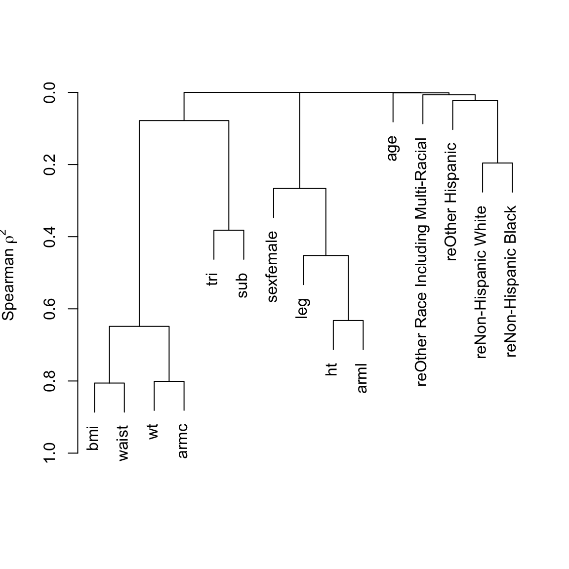

Figure 15.6: Variable clustering for all potential predictors

Six size measures adequately capture the entire set. Height and BMI are removed. An advantage of removing height is that it is age-dependent in the elderly:

Z

f <- orm(ht ~ rcs(age,4)*sex, data=w)  # Prop. odds model
qu <- Quantile(f); med <- function(x) qu(.5, x)
ggplot(Predict(f, age, sex, fun=med, conf.int=FALSE),
       ylab='Predicted Median Height, cm')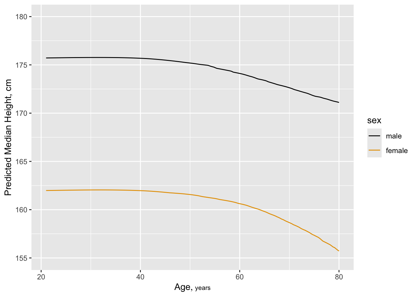

Figure 15.7: Estimated median height as a smooth function of age, allowing age to interact with sex, from a proportional odds model

But also see a change in leg length:

f <- orm(leg ~ rcs(age,4)*sex, data=w)
qu <- Quantile(f); med <- function(x) qu(.5, x)
ggplot(Predict(f, age, sex, fun=med, conf.int=FALSE),
       ylab='Predicted Median Upper Leg Length, cm')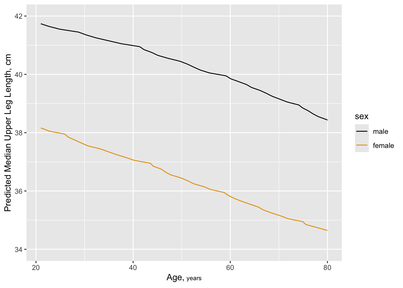

Figure 15.8: Estimated median upper leg length as a smooth function of age, allowing age to interact with sex, from a proportional odds model

Next allocate d.f. according to generalized Spearman
\(\rho^{2}\) ⁹.

A

⁹ Competition between collinear size measures hurts interpretation of partial tests of association in a saturated additive model.

spar(top=1, ps=9)
s <- spearman2(gh ~ age + sex + re + wt + leg + arml + armc +
               waist + tri + sub, data=w, p=2)
plot(s)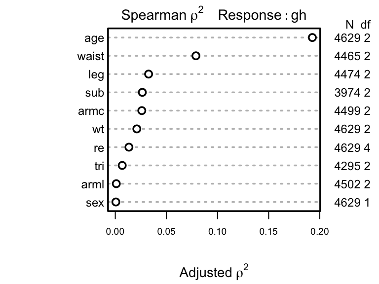

Figure 15.9: Generalized squared rank correlations

Parameters will be allocated in descending order of \(\rho^2\). But note that subscapular skinfold has a large number of NAs and other predictors also have NAs. Suboptimal casewise deletion will be used until the final model is fitted. Because there are many competing body measures, we use backwards stepdown to arrive at a set of predictors. The bootstrap will be used to penalize predictive ability for variable selection. First the full model is fit using casewise deletion, then we do a composite test to assess whether any of the frequently-missing predictors is important. Use likelihood ratio \(\chi^2\) tests.

B

f <- orm(gh ~ rcs(age,5) + sex + re + rcs(wt,3) + rcs(leg,3) + arml +
         rcs(armc,3) + rcs(waist,4) + tri + rcs(sub,3),
         family='loglog', data=w, x=TRUE, y=TRUE)
print(f, coefs=FALSE)

-log-log Ordinal Regression Model

orm(formula = gh ~ rcs(age, 5) + sex + re + rcs(wt, 3) + rcs(leg, 
    3) + arml + rcs(armc, 3) + rcs(waist, 4) + tri + rcs(sub, 
    3), data = w, family = "loglog", x = TRUE, y = TRUE)

	Model Likelihood Ratio Test	Discrimination Indexes	Rank Discrim. Indexes
Obs 3853	LR χ2 1180.13	R2 0.265	ρ 0.520
ESS 3829.2	d.f. 22	R222,3853 0.260	Dxy 0.388
Distinct Y 60	Pr(>χ2) <0.0001	R222,3829.2 0.261
Y0.5 5.5	Score χ2 1298.88	|Pr(Y ≥ median)-½| 0.172
max |∂log L/∂β| 7×10-11	Pr(>χ2) <0.0001

## Composite test:
anova(f, leg, arml, armc, waist, tri, sub, test='LR')

Likelihood Ratio Statistics for gh
	χ2	d.f.	P
leg	8.44	2	0.0147
Nonlinear	3.36	1	0.0668
arml	0.16	1	0.6925
armc	6.63	2	0.0364
Nonlinear	3.27	1	0.0707
waist	29.48	3	<0.0001
Nonlinear	4.30	2	0.1165
tri	16.50	1	<0.0001
sub	41.53	2	<0.0001
Nonlinear	4.53	1	0.0334
TOTAL NONLINEAR	15.04	5	0.0102
TOTAL	130.04	11	<0.0001

The model yields Spearman \(\rho=0.52\), the rank correlation between predicted and observed \(\text{HbA}_{1c}\). Show predicted mean and median \(\text{HbA}_{1c}\) as a function of age, adjusting other variables to median/mode. Compare the estimate of the median with that from quantile regression (discussed below).

C

M      <- Mean(f)
qu     <- Quantile(f)
med    <- function(x) qu(.5, x)
p90    <- function(x) qu(.9, x)
fq     <- Rq(formula(f), data=w)
fq90   <- Rq(formula(f), data=w, tau=.9)
pmean  <- Predict(f,    age, fun=M,   conf.int=FALSE)
pmed   <- Predict(f,    age, fun=med, conf.int=FALSE)
p90    <- Predict(f,    age, fun=p90, conf.int=FALSE)
pmedqr <- Predict(fq,   age, conf.int=FALSE)
p90qr  <- Predict(fq90, age, conf.int=FALSE)
z <- rbind('orm mean'=pmean, 'orm median'=pmed, 'orm P90'=p90,
           'QR median'=pmedqr, 'QR P90'=p90qr)
ggplot(z, groups='.set.',
       adj.subtitle=FALSE, legend.label=FALSE)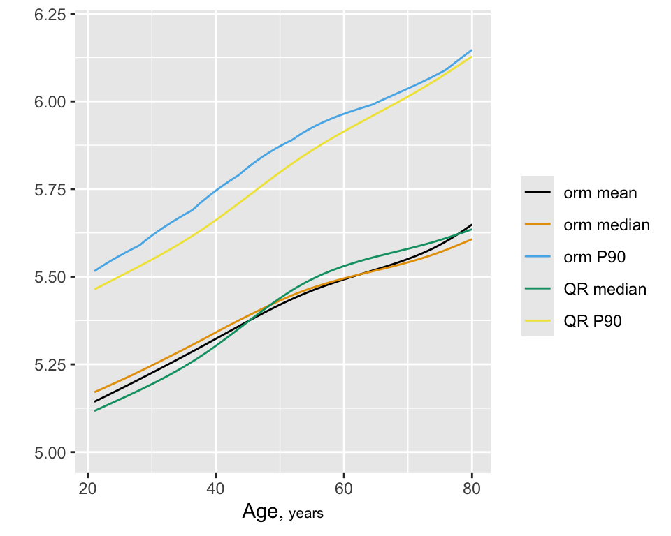

Figure 15.10: Estimated mean and 0.5 and 0.9 quantiles from the log-log ordinal model using casewise deletion, along with predictions of 0.5 and 0.9 quantiles from quantile regression (QR). Age is varied and other predictors are held constant to medians/modes.

Next do fast backward step-down in an attempt to get a model without so much competition among variables. The stepwise selection will be penalized for in the model validation.

D

print(fastbw(f, rule='p'), estimates=FALSE)

 Deleted Chi-Sq d.f. P      Residual d.f. P      AIC  
 arml    0.16   1    0.6924 0.16     1    0.6924 -1.84
 sex     0.45   1    0.5019 0.61     2    0.7381 -3.39
 wt      5.72   2    0.0572 6.33     4    0.1759 -1.67
 armc    3.32   2    0.1897 9.65     6    0.1400 -2.35

Factors in Final Model

[1] age   re    leg   waist tri   sub  

Validate the model, properly penalizing for variable selection

E

g <- function() {
  set.seed(13)  # so can reproduce results
  validate(f, B=100, bw=TRUE, estimates=FALSE, rule='p')
}
v <- runifChanged(g)

# Show number of variables selected in first 30 boots
print(v, B=30)

Index	Original Sample	Training Sample	Test Sample	Optimism	Corrected Index	Successful Resamples
ρ	0.5172	0.5209	0.5149	0.006	0.5112	100
Dxy	0.3861	0.3893	0.3842	0.005	0.3811	100
R2	0.2629	0.2686	0.2592	0.0094	0.2535	100
Slope	1	1	0.9772	0.0228	0.9772	100
g	0.7289	0.7401	0.7218	0.0183	0.7106	100
Mean |Pr(Y≥Y0.5)-0.5|	0.172	0.176	0.1702	0.0058	0.1662	100

Factors Retained in Backwards Elimination First 30 Resamples
age	sex	re	wt	leg	arml	armc	waist	tri	sub
⚬		⚬		⚬	⚬	⚬	⚬	⚬	⚬
⚬	⚬	⚬	⚬	⚬		⚬	⚬	⚬	⚬
⚬		⚬	⚬			⚬	⚬	⚬	⚬
⚬		⚬		⚬			⚬	⚬	⚬
⚬		⚬		⚬			⚬	⚬	⚬
⚬		⚬		⚬		⚬	⚬	⚬	⚬
⚬		⚬	⚬	⚬		⚬	⚬	⚬	⚬
⚬		⚬		⚬			⚬	⚬	⚬
⚬		⚬	⚬			⚬	⚬	⚬	⚬
⚬		⚬	⚬			⚬	⚬	⚬	⚬
⚬		⚬		⚬			⚬	⚬	⚬
⚬		⚬	⚬			⚬	⚬	⚬	⚬
⚬		⚬		⚬			⚬	⚬	⚬
⚬		⚬		⚬			⚬	⚬	⚬
⚬		⚬	⚬			⚬	⚬	⚬	⚬
⚬		⚬	⚬			⚬	⚬	⚬	⚬
⚬		⚬	⚬	⚬		⚬	⚬	⚬	⚬
⚬		⚬		⚬		⚬	⚬	⚬	⚬
⚬		⚬	⚬			⚬	⚬	⚬	⚬
⚬	⚬	⚬		⚬			⚬	⚬	⚬
⚬		⚬	⚬			⚬	⚬	⚬	⚬
⚬		⚬	⚬	⚬		⚬	⚬	⚬	⚬
⚬		⚬	⚬	⚬		⚬	⚬	⚬	⚬
⚬		⚬	⚬	⚬		⚬	⚬	⚬	⚬
⚬		⚬	⚬			⚬	⚬	⚬	⚬
⚬		⚬	⚬	⚬			⚬	⚬	⚬
⚬		⚬	⚬				⚬	⚬	⚬
⚬		⚬		⚬			⚬	⚬	⚬
⚬		⚬	⚬				⚬	⚬	⚬
⚬		⚬		⚬			⚬	⚬	⚬

Frequencies of Numbers of Factors Retained
5	6	7	8	9
1	33	41	21	4

Develop multiple imputations then repeat the bootstrap validation process, but separately for each completed dataset. The overall validation averages the bootstrap-corrected model performance measures over five validations.

set.seed(11)
a <- aregImpute(~ gh + age + sex + re + wt + leg + arml + armc + waist +
                  tri + sub, data=w, n.impute=5, pr=FALSE)
a

Multiple Imputation using Bootstrap and PMM

aregImpute(formula = ~gh + age + sex + re + wt + leg + arml + 
    armc + waist + tri + sub, data = w, n.impute = 5, pr = FALSE)

n: 4629     p: 11   Imputations: 5      nk: 3 

Number of NAs:
   gh   age   sex    re    wt   leg  arml  armc waist   tri   sub 
    0     0     0     0     0   155   127   130   164   334   655 

      type d.f.
gh       s    2
age      s    2
sex      c    1
re       c    4
wt       s    2
leg      s    2
arml     s    2
armc     s    2
waist    s    2
tri      s    2
sub      s    1

Transformation of Target Variables Forced to be Linear

R-squares for Predicting Non-Missing Values for Each Variable
Using Last Imputations of Predictors
  leg  arml  armc waist   tri   sub 
0.638 0.720 0.862 0.904 0.746 0.641 

v <- function(fit)
  list(validate=validate(fit, B=100, bw=TRUE, estimates=FALSE, 
                         prmodsel=FALSE, rule='p', pr=FALSE))
h <- function()
  fit.mult.impute(gh ~ rcs(age,5) + sex + re + rcs(wt,3) + rcs(leg,3) + arml +
                  rcs(armc,3) + rcs(waist,4) + tri + rcs(sub,3),
                  orm, a, data=w,
                  fun=v, fitargs=list(x=TRUE, y=TRUE, family='loglog'), pr=FALSE)
f <- runifChanged(h, a, v)  # 11m
print(processMI(f, 'validate'), B=10, digits=3)

Index	Original Sample	Training Sample	Test Sample	Optimism	Corrected Index	Successful Resamples
ρ	0.513	0.515	0.511	0.004	0.508	500
Dxy	0.384	0.386	0.382	0.004	0.38	500
R2	0.268	0.273	0.266	0.007	0.261	500
Slope	1	1	0.981	0.019	0.981	500
g	0.741	0.749	0.734	0.015	0.726	500
Mean |Pr(Y≥Y0.5)-0.5|	0.173	0.174	0.171	0.003	0.17	500

Factors Retained in Backwards Elimination First 10 Resamples
age	sex	re	wt	leg	arml	armc	waist	tri	sub
⚬		⚬	⚬	⚬		⚬	⚬	⚬	⚬
⚬		⚬	⚬	⚬		⚬	⚬	⚬	⚬
⚬		⚬					⚬	⚬	⚬
⚬		⚬	⚬			⚬	⚬	⚬	⚬
⚬		⚬		⚬			⚬	⚬	⚬
⚬	⚬	⚬		⚬			⚬	⚬	⚬
⚬		⚬	⚬			⚬	⚬	⚬	⚬
⚬	⚬	⚬	⚬	⚬		⚬	⚬	⚬	⚬
⚬		⚬	⚬			⚬	⚬	⚬	⚬
⚬		⚬	⚬	⚬	⚬	⚬	⚬	⚬	⚬

Frequencies of Numbers of Factors Retained
5	6	7	8	9	10
1	38	31	22	7	1

There is no calibrate method for orm model fits.

Next fit the reduced model. Use multiple imputation to impute missing predictors. Do a LR ANOVA for the reduced model, taking imputation into account.

FG

h <- function()
  fit.mult.impute(gh ~ rcs(age,5) + re + rcs(leg,3) +
                       rcs(waist,4) + tri + rcs(sub,4),
                  orm, a, fitargs=list(family='loglog'),
                  lrt=TRUE,
                  data=w, pr=FALSE)
g <- runifChanged(h, a)
g

-log-log Ordinal Regression Model

fit.mult.impute(formula = gh ~ rcs(age, 5) + re + rcs(leg, 3) + 
    rcs(waist, 4) + tri + rcs(sub, 4), fitter = orm, xtrans = a, 
    data = w, lrt = TRUE, pr = FALSE, fitargs = list(family = "loglog"))

	Model Likelihood Ratio Test	Discrimination Indexes	Rank Discrim. Indexes
Obs 4629	LR χ2 1443.45	R2 0.269	ρ 0.512
ESS 23011.2	d.f. 17	R217,23145 0.267	Dxy 0.383
Distinct Y 63	Pr(>χ2) <0.0001	R217,23011.2 0.269
Y0.5 5.5	Score χ2 7820.99	|Pr(Y ≥ median)-½| 0.173
max |∂log L/∂β| 1×10-10	Pr(>χ2) <0.0001

	β	S.E.	Wald Z	Pr(>|Z|)
age	0.0405	0.0055	7.35	<0.0001
age'	-0.0226	0.0277	-0.82	0.4146
age''	0.0114	0.0871	0.13	0.8958
age'''	0.0448	0.1145	0.39	0.6958
re=Other Hispanic	-0.0703	0.0592	-1.19	0.2345
re=Non-Hispanic White	-0.4128	0.0450	-9.18	<0.0001
re=Non-Hispanic Black	0.0635	0.0562	1.13	0.2589
re=Other Race Including Multi-Racial	-0.0434	0.0746	-0.58	0.5607
leg	-0.0324	0.0092	-3.51	0.0004
leg'	0.0138	0.0107	1.28	0.1988
waist	0.0076	0.0050	1.52	0.1283
waist'	0.0305	0.0161	1.90	0.0576
waist''	-0.0916	0.0522	-1.76	0.0790
tri	-0.0159	0.0026	-6.04	<0.0001
sub	-0.0026	0.0097	-0.27	0.7881
sub'	0.0635	0.0307	2.07	0.0386
sub''	-0.1694	0.0999	-1.70	0.0898

an <- processMI(g, 'anova')
# Show penalty-type parameters for imputation
prmiInfo(an)

Imputation penalties
Test	Missing Information Fraction	Denominator d.f.	χ2 Discount
age	0.095	1760.5	0.905
Nonlinear	0.033	11155.4	0.967
re	0.000	Inf	1.000
leg	0.003	914800.9	0.997
Nonlinear	0.071	788.9	0.929
waist	0.000	Inf	1.000
Nonlinear	0.030	8609.4	0.970
tri	0.155	166.0	0.845
sub	0.301	132.9	0.699
Nonlinear	0.286	98.0	0.714
TOTAL NONLINEAR	0.100	3197.8	0.900
TOTAL	0.074	12487.9	0.926

# Correct likelihood-based statistics for imputation
g <- LRupdate(g, an)
print(an, caption='ANOVA for reduced model after multiple imputation, with addition of a combined effect for four size variables')

ANOVA for reduced model after multiple imputation, with addition of a combined effect for four size variables
	χ2	d.f.	P
age	630.21	4	<0.0001
Nonlinear	28.12	3	<0.0001
re	172.14	4	<0.0001
leg	24.25	2	<0.0001
Nonlinear	1.64	1	0.2009
waist	152.89	3	<0.0001
Nonlinear	3.87	2	0.1442
tri	33.22	1	<0.0001
sub	36.85	3	<0.0001
Nonlinear	5.28	2	0.0714
TOTAL NONLINEAR	42.48	8	<0.0001
TOTAL	1336.94	17	<0.0001

b  <- anova(g, leg, waist, tri, sub)
# Add new lines to the plot with combined effect of 4 size var.
s <- rbind(an, size=b['TOTAL', ])
class(s) <- 'anova.rms'

spar(top=1)
plot(s)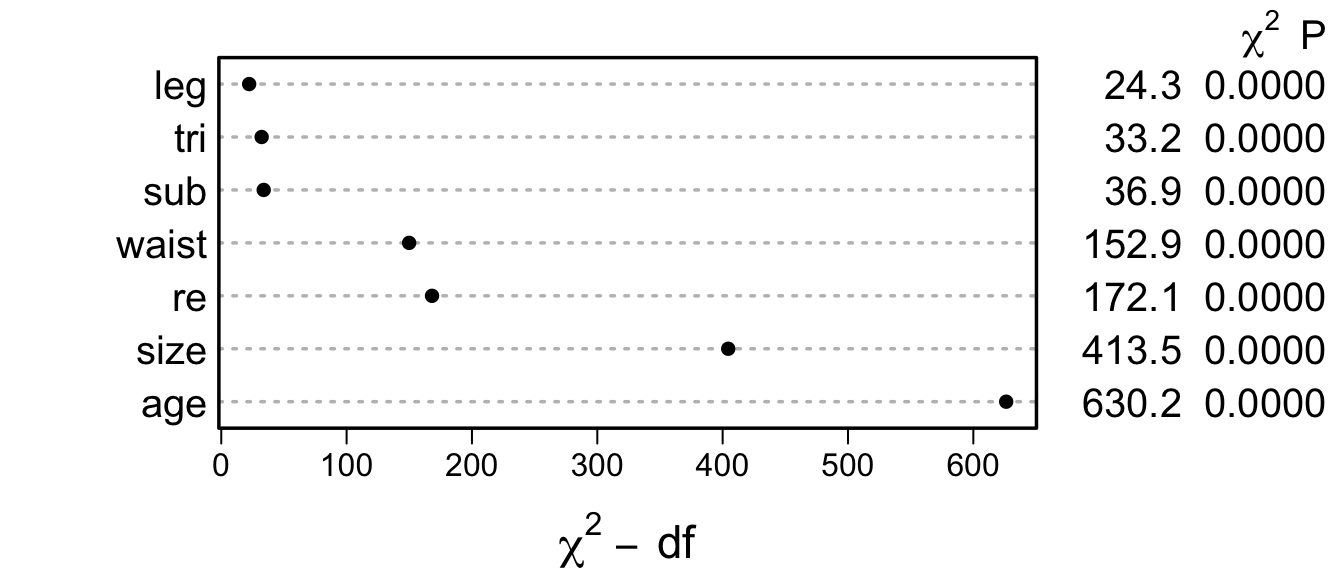

Figure 15.11: ANOVA for reduced model after multiple imputation

H

ggplot(Predict(g), abbrev=TRUE, ylab=NULL)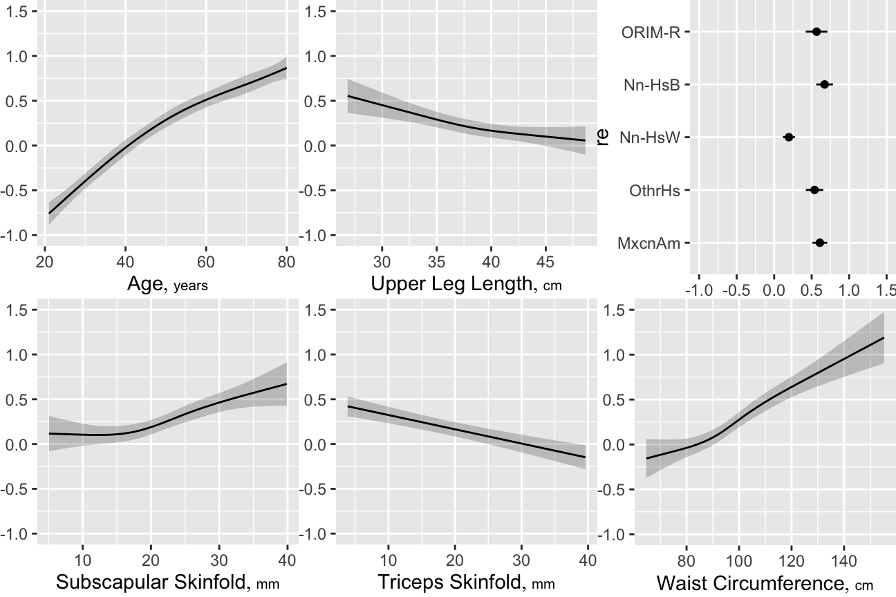   

Figure 15.12: Partial effects (log hazard or log-log cumulative probability scale) of all predictors in reduced model, after multiple imputation

I

M <- Mean(g)
ggplot(Predict(g, fun=M), abbrev=TRUE, ylab=NULL)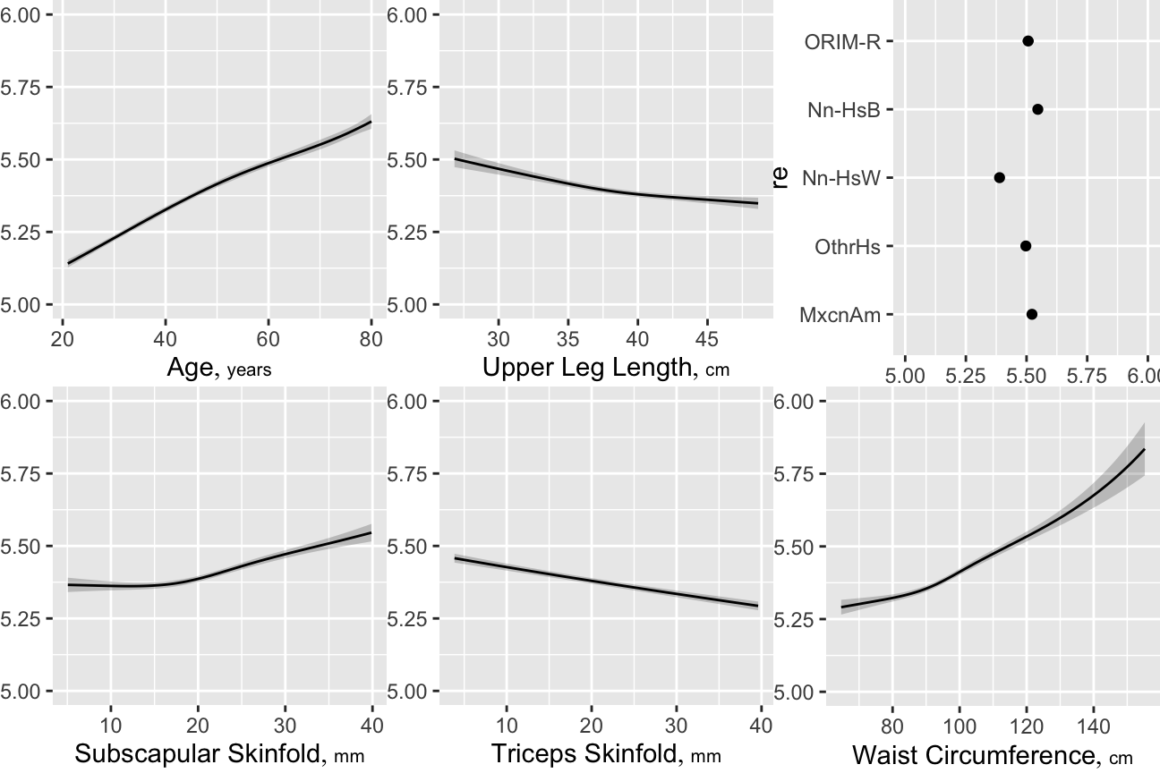   

Figure 15.13: Partial effects (mean scale) of all predictors in reduced model, after multiple imputation

Compare the estimated age partial effects and confidence intervals with those from a model using casewise deletion, and with bootstrap nonparametric confidence intervals (also with casewise deletion).

J

h <- function() {
  gc <- orm(gh ~ rcs(age,5) + re + rcs(leg,3) +
            rcs(waist,4) + tri + rcs(sub,4),
            family='loglog', data=w, x=TRUE, y=TRUE)
  gb <- bootcov(gc, B=300)
  list(gc=gc, gb=gb)
}
gbc <- runifChanged(h)
gc  <- gbc$gc
gb  <- gbc$gb

pgc     <- Predict(gc, age)
bootclb <- Predict(gb, age, boot.type='basic')
bootclp <- Predict(gb, age, boot.type='percentile')
multimp <- Predict(g,  age)
p <- rbind('casewise deletion'    = pgc,
           'basic bootstrap'      = bootclb,
           'percentile bootstrap' = bootclp,
           'multiple imputation'  = multimp)[, .q(age, yhat, lower, upper, .set.)]
m <- melt(as.data.table(p), id.vars=c('age', '.set.'))

ggplot(m, aes(x=age, y=value, color=.set.,
              group=paste(variable, .set.))) + geom_line() +
  guides(color=guide_legend(title='')) +
  theme(legend.position='bottom') +
  ylab(expression(X * hat(beta)))

Figure 15.14: Partial effect for age from multiple imputation and casewise deletion (center lines with the green line depicting all non-multiple-imputation methods) with symmetric Wald 0.95 confidence bands using casewise deletion, basic bootstrap confidence bands using casewise deletion, percentile bootstrap confidence bands using casewise deletion, and symmetric Wald confidence bands accounting for multiple imputation.

In OLS the mean equals the median and both are linearly related to any other quantiles. Semiparametric models are not this restrictive:

K

M  <- Mean(g)
qu <- Quantile(g)
med <- function(lp) qu(.5, lp)
q90 <- function(lp) qu(.9, lp)
lp  <- predict(g)
lpr <- quantile(predict(g), c(.002, .998), na.rm=TRUE)
lps <- seq(lpr[1], lpr[2], length=200)
pmn <- M(lps)
pme <- med(lps)
p90 <- q90(lps)
plot(pmn, pme,   
     xlab=expression(paste('Predicted Mean ',  HbA["1c"])),
     ylab='Median and 0.9 Quantile', type='l',
     xlim=c(4.75, 8.0), ylim=c(4.75, 8.0), bty='n')
box(col=gray(.8))
lines(pmn, p90, col='blue')
abline(a=0, b=1, col=gray(.8))
text(6.5, 5.5, 'Median')
text(5.5, 6.3, '0.9', col='blue')
nint <- 350
scat1d(M(lp),   nint=nint)
scat1d(med(lp), side=2, nint=nint)
scat1d(q90(lp), side=4, col='blue', nint=nint)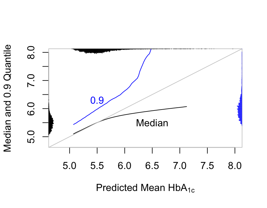

Figure 15.15: Predicted mean r hba vs. predicted median and 0.9 quantile along with their marginal distributions

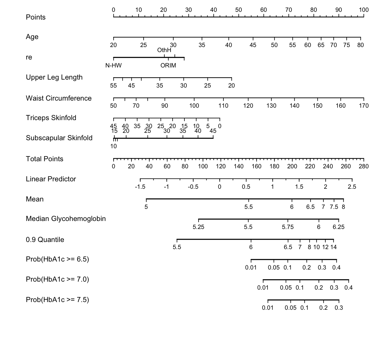
Draw a nomogram to compute 7 different predicted values for each subject.

L

spar(ps=9)
g      <- Newlevels(g, list(re=abbreviate(levels(w$re))))
exprob <- ExProb(g)
nom <-
  nomogram(g, fun=list(Mean=M,
                'Median Glycohemoglobin' = med,
                '0.9 Quantile'           = q90,
                'Prob(HbA1c >= 6.5)'=
                     function(x) exprob(x, y=6.5),
                'Prob(HbA1c >= 7.0)'=
                     function(x) exprob(x, y=7),
                'Prob(HbA1c >= 7.5)'=
                     function(x) exprob(x, y=7.5)),
           fun.at=list(seq(5, 8, by=.5),
             c(5,5.25,5.5,5.75,6,6.25),
             c(5.5,6,6.5,7,8,10,12,14),
             c(.01,.05,.1,.2,.3,.4),
             c(.01,.05,.1,.2,.3,.4),
             c(.01,.05,.1,.2,.3,.4)))
plot(nom, lmgp=.28)   

Figure 15.16: Nomogram for predicting median, mean, and 0.9 quantile of glycohemoglobin, along with the estimated probability that \(\text{HbA}_{1c} \ge 6.5, 7\), or \(7.5\), all from the log-log ordinal model

Centers for Disease Control and Prevention CDC. National Center for Health Statistics NCHS. (2010). National Health and Nutrition Examination Survey. http://www.cdc.gov/nchs/nhanes/nhanes2009-2010/nhanes09_10.htm

Kalbfleisch, J. D., & Prentice, R. L. (1973). Marginal likelihood based on Cox’s regression and life model. Biometrika, 60, 267–278.

Koenker, R. (2005). Quantile Regression. Cambridge University Press.

Koenker, R. (2009). Quantreg: Quantile Regression. http://CRAN.R-project.org/package=quantreg

Koenker, R., & Bassett, G. (1978). Regression quantiles. Econometrica, 46, 33–50.

Manuguerra, M., & Heller, G. Z. (2010). Ordinal Regression Models for Continuous Scales. Int J Biostat, 6(1). https://doi.org/10.2202/1557-4679.1230

mislabeled a flexible parametric model as semi-parametric; does not cover semi-parametric approach with lots of intercepts

Venables, W. N., & Ripley, B. D. (2003). Modern Applied Statistics with S (Fourth). Springer-Verlag.