25 Ordinal Semiparametric Regression for Survival Analysis
25.1 Background
This chapter considers methods for typical survival analyses used for analyzing time until a single type of event occurs, without competing risks. Most applications involve right-censoring, to handle subjects who have not been followed long enough to have an event observed.
The most popular methods used in this setting are the Kaplan-Meier survival curve estimator for homogeneous groups, and the Cox proportional hazards (PH) model for modeling covariates and also possibly including strata whose effects are not parameterized but which induce differently-shaped survival curves.
This can be thought of as providing adjusted Kaplan-Meier curves
The Cox PH model uses the marginal distribution of ranks of failure times that come from an underlying Gumbel extreme-value distribution \(\exp(-\exp(t))\). This gives rise to proportional hazards effects of covariates, and the Cox partial likelihood that does not involve the underlying hazard or survival curve for a “standard” subject, e.g., a subject with all covariates equal to their mean. This implies that maximum partial likelihood estimates can be calculated very quickly without dealing with intercepts in the model. But the extreme value distribution is the only distribution for which the multi-dimensional integration that results in the marginal likelihood is tractable. That isolates Cox PH from all the other survival model forms that cannot use partial likelihood.
Instead of seeking partial likelihood solutions, full semiparametric likelihoods can be used. That allows extension of the Cox model semiparametric theme to any distribution, because with semiparametric models the intercepts are estimated simultaneously with \(\beta\). Sparse matrix operations allow full maximum likelihood iterative calculations and matrix operations to be as fast as using the Cox partial likelihood, so some of the issues that originally motivated the Cox model are moot. And unlike the Cox model, semiparametric ordinal models handle left- and interval-censoring. As will be seen below, ordinal models also unite PH and accelerated failure time (AFT) models. In essence, one ordinal model encompasses all of single-event-type survival analysis, with different link function choices giving rise to the complete PH-AFT spectrum and beyond. For AFT, ordinal models have an incredibly important advantage of not assuming a specific transformation of time, such as the commonly used \(\log(t)\) transformation that gives rise to log-logistic, log-normal, and log-\(t\) survival models when for example the residuals actually follow logistic, normal, or \(t\) distributions.
25.2 Cumulative Probability Models
Cumulative probability ordinal models (CPMs) are natural for survival analysis. For a distribution family \(F\) the usual model
\[ P(Y \geq y | X) = F(\alpha_{y} + X\beta) \]
automatically provides the survival function
\[ S(t | X) = P(T > t | X) = F(\alpha_{t+} + X\beta) \]
where \(\alpha_{t+}\) is the next intercept after \(\alpha_t\).
25.2.1 Interpretation of Parameters
Consider a predictor \(X_{j}\) that operates linearly and does not interact with any other predictor. A one-unit change in \(X_{j}\) then changes the linear predictor \(X\beta\) by \(\beta_{j}\) units. Equivalently, it changes \(F^{-1}(S(t | X))\) by \(\beta_j\) units. For some link functions, the interpretation can be stated in other ways, letting \(r = \exp(\beta_{j})\) denote an effect ratio.
- logit link: \(r\) is a survival odds ratio, i.e., \(\frac{\text{odds}(T > t | X=a+1)}{\text{odds}(T > t | X=a)}\), where \(\text{odds}(u) = \frac{P(u)}{1 - P(u)}\), \(a\) is any constant, and \(u\) represents some assertion
- log-log link: \(r\) is the exponent relating the two survival curves, i.e., \(S(T > t | X=a+1) = S(T > t | X=a)^{r}\). In the special case that \(T\) is truly continuous, i.e., the distance between successive distinct values of \(T\) goes to zero as \(n \rightarrow \infty\), \(\frac{1}{r}\) is the \(X=a+1 : X=a\) hazard ratio and the model is a proportional hazards model. The hazard ratio is \(\exp(-\beta_{j})\). The idea of a continuous hazard function (and hence ratios of them) does not apply when \(T\) is really discrete.
- complementary log-log link: \(r\) is the exponent relating \((1 - S(t | X=a+1))\) to \((1 - S(t | X=a))\), i.e., the cumulative distribution functions or cumulative incidence functions \(C(t | X) = 1 - S(t | X)\). \(C(t | X=a+1) = C(t | X=a)^{r}\).
The probit link is harder to interpret. \(\beta_j\) is a “\(z\)-score change.”
25.2.2 CPMs and Censoring
Consider any semiparametric regression model in the class of cumulative probability models. It is easy to modify the likelihood function for such a model to make optimum use of incomplete dependent variable information due to left, right, and interval censoring. The rms package orm function starting with version 8.0 handles these censoring patterns. The rms Ocens function is used instead of the survival package Surv function, to specify censoring details and to package the results in a 2-column matrix. Ocens takes two numeric variables a, b. For a complete observation, a=b. For a left-censored observation, a is \(-\infty\), coded in r as -Inf and b is finite. For a right-censored observation, a is finite and b is \(\infty\), coded as Inf. For example, an observation that is right-censored at 2 years may be coded as (2, Inf). An interval censored observation has both a and b numeric but b > a. This is considered to be a closed interval inclusive of the endpoints. Left- and right-censored intervals are assumed to be exclusive, e.g., (2, Inf) stands for “we know that the true event time is greater than 2”.
The rms orm function takes a user-specified Ocens object and runs it through the Ocens2ord function to do the recoding into a discrete ordinal variable. If there is no censoring, the response variable Y is simply recoded to an integer vector based on the unique (to within \(10^{-7}\) by default) values occurring in the data. For left- or right- censoring, censored values are recoded to the next inward uncensored value and considered censored at that open-interval value. All censored values that are beyond the outermost uncensored values are coded at the innermost censored value that is beyond the most extreme uncensored value, and a new uncensored category is created at this value. For right censoring, this process makes the maximum likelihood estimates (MLE) of the model intercepts, when there no covariates, exactly equal to the link function of Kaplan-Meier estimates. When the highest coded value is right-censored at say a value \(y\), the predicted value of \(P(Y \geq y)\) will be greater than 0, so the resulting survival curve will not be observed to drop to zero. If the highest observation is uncensored, the estimated survival curve will drop to zero at that point.
For interval censoring, the process of converting general intervals to ordered categories is a complex one involving Turnbull intervals (maximal intersections of the censoring intervals). Some Turnbull intervals may carry no estimable probability, which would otherwise cause orm to compute an invalid likelihood; Ocens2ord detects and consolidates these using the Kuhn-Tucker (self-consistency) condition of the nonparametric maximum likelihood estimate, computed by an internal Turnbull self-consistency algorithm implemented in base R. Ocens2ord has two algorithms for interval consolidation: the default, cons='intervals', remaps interval definitions without changing the data; a deprecated legacy alternative, cons='data', instead iteratively widens the raw data values and requires the icenReg package. Except in rare situations such as having certain patterns of tied times in the data, the MLEs are exactly the Turnbull nonparametric interval-censored survival probability estimates transformed by the link function.
Related resources and important background publications by several authors may be found here.
25.3 Special Cases of Ordinal Cumulative Probability Models

There are important implications of the generality, robustness, and efficiency of ordinal regression for censored data just as there are for uncensored data. The generality of cumulative probability models (CPMs) allows them to bridge binary, discrete, and continuous ordinal regression to survival analysis and simple statistical tests, and would present major didactic simplifications for statistics courses. Ordinal regression covers all the following special cases:
- An ordinal regression with logit link and only 2 Y levels is binary logistic regression
- The score test in binary logistic regression is the Pearson \(\chi^2\) test
- The score test in proportional odds regression is the Wilcoxon statistic
- The score test in a log-log link ordinal model is the logrank statistic
- Ordinal regression for continuous Y with a probit link essentially has the linear model as a special case without needing to know how to transform Y for modeling
- When there is only right censoring and no covariates, the estimated survival curve from ordinal regression is exactly the Kaplan-Meier estimate
- The link function is irrelevant for the survival point estimates
- Different link functions will give rise to different confidence intervals
- Example: A log-log link gives identical confidence intervals to Kaplan-Meier intervals using the standard error of log-log survival
- For interval-censored data, survival estimates with no covariates are almost exactly Turnbull estimates
- Parametric accelerated failure time models are special cases of ordinal models with probit or logit links
- they are special cases because they assume that time is correctly transformed (it is usually logged) to make the residuals have a specific distribution
- normal survival time model is a special case of a probit ordinal model where the intercepts are linearly related to the times they represent
- log-normal survival time model is a special case of a probit model with intercepts as linear functions of log time
- The ordinal model provides results that are independent of any time transformation that is monotonically increasing
- The Cox PH model is a special case of an ordinal model with a log-log link. Cox (1972) developed a partial likelihood approach to make estimation of regression coefficients very easy and fast. This approach required the intercepts (underlying survival curve) to be estimated in a second step once \(\hat{\beta}\) were computed. There is a degree of arbitrariness in this approach, and methods for computing confidence intervals for estimated survival probabilities are complex. Ordinal models use full likelihood so they estimate the intercepts simultaneously with \(\beta\). This is about as fast as just estimating \(\beta\) with Cox PH, because with right censoring the hessian matrix for ordinal models is extremely sparse, so inverting its negative in order to get the covariance matrix is extremely fast even with hundreds of thousands of distinct failure times.
For score tests see Section 9.2, here and here. The numerator of a score statistic is the first derivative of the log-likelihood evaluated at the null parameter value. It is an “observed - expected” quantity.
NoteAgreement of Cox Model and Ordinal Regression
- Simulate many random datasets with \(n\) varying from 10 to 500
- one run per \(n\)
- Compare ordinal model with log-log link maximum likelihood estimates to Cox maximum partial likelihood exact estimates
- \(\hat{\beta}\) from ordinal model is negated to make it comparable
- Also compare standard errors and whether ordinal estimates are closer to exact Cox estimates than to Efron approximate estimates
Code
sim <- function(n) {
  x    <- runif(n)
  y    <- sample(n, replace=TRUE) + round(n * x / 2)
  cens <- sample(floor(n / 3) : n, n, replace=TRUE)
  ev   <- y <= cens
  # tied <- sum(duplicated(y[ev]))
  f1   <- cph(Surv(y, ev) ~ x, method='exact')
  f2   <- cph(Surv(y, ev) ~ x, method='efron')
  c1   <- coef(f1)
  c2   <- coef(f2)
  Y    <- Ocens(y, ifelse(ev, y, Inf))
  g    <- orm(Y ~ x, family='loglog')
  o    <- - coef(g)[length(coef(g))]
  s1   <- sqrt(vcov(f1))
  s2   <- sqrt(vcov(f2))
  so   <- sqrt(vcov(g, intercepts='none'))
  Nu   <- sum(ev)
  foldchange <- function(a, b) {
    r <- abs(log(a / b))
    exp(r)
  }
  list(method = c('Ordinal:Cox exact', 'Ordinal:Cox Efron'),
       beta   = c(abs(o - c1),          abs(o - c2)),
       sbeta  = c(abs(o - c1) / s1,     abs(o - c2) / s2),
       se     = c(foldchange(so, s1),   foldchange(so, s2)),
       closer = c(abs(o - c1) <= abs(c1 - c2), NA),
       Nu     = rep(Nu, 2) )
}
set.seed(11)
R <- expand.grid(n=10:500)
setDT(R)   # make it a data.table
w <- R[, sim(n), by=.(n)]
xl <- xlab(expression(n))
ggplot(w, aes(x=n, y=beta, color=method)) + geom_point() +
  xl + ylab(expression(abs(Delta~hat(beta))))
ggplot(w, aes(x=n, y=sbeta, color=method)) + geom_point() +
  xl + ylab(expression(paste('Difference in ', hat(beta), ' in S.E. Units')))
ggplot(w, aes(x=n, y=se, color=method)) + geom_point() +
  scale_y_continuous(transform='log',
                     breaks=c(1, 1.001, 1.005, 1.01, 1.02, 1.05, 1.1, 1.15)) +
  xl + ylab('Ratio of S.E.')
m <- movStats(closer ~ n, data=w, loess=TRUE, melt=TRUE)
# Moving overlapping windows to estimate smooth trend:
ggplot(m, aes(x=n, y=closer, color=Type)) + geom_line() +
  xl + ylab(expression(paste('Proportion Ordinal Closer Than Efron to Exact ', hat(beta))))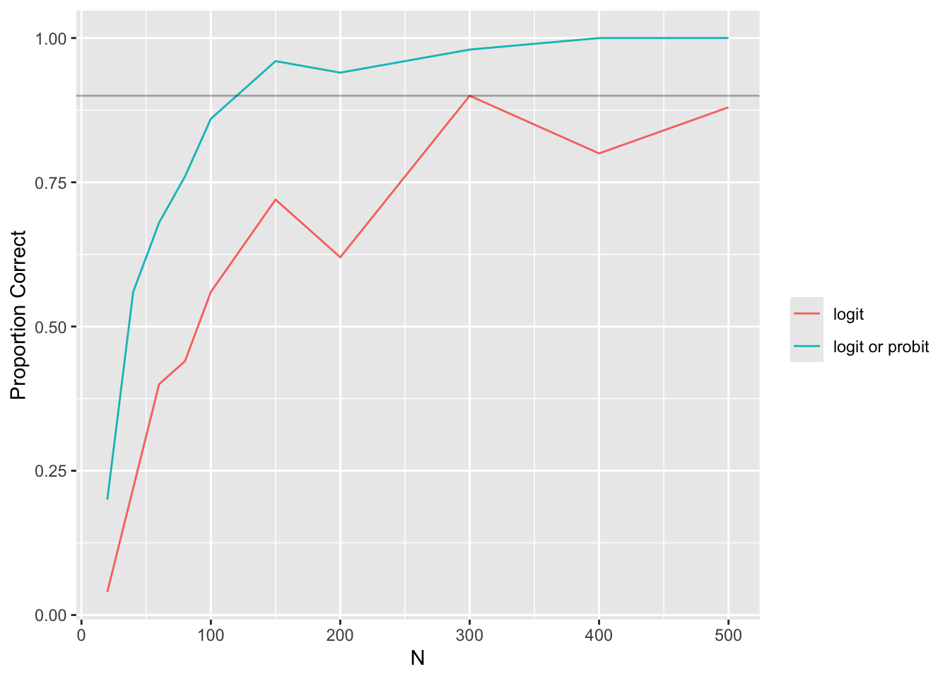
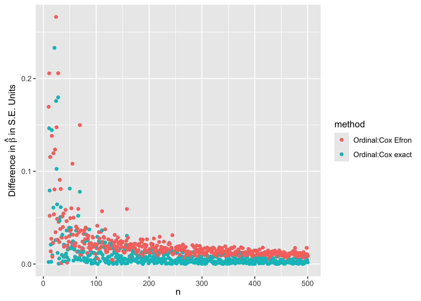
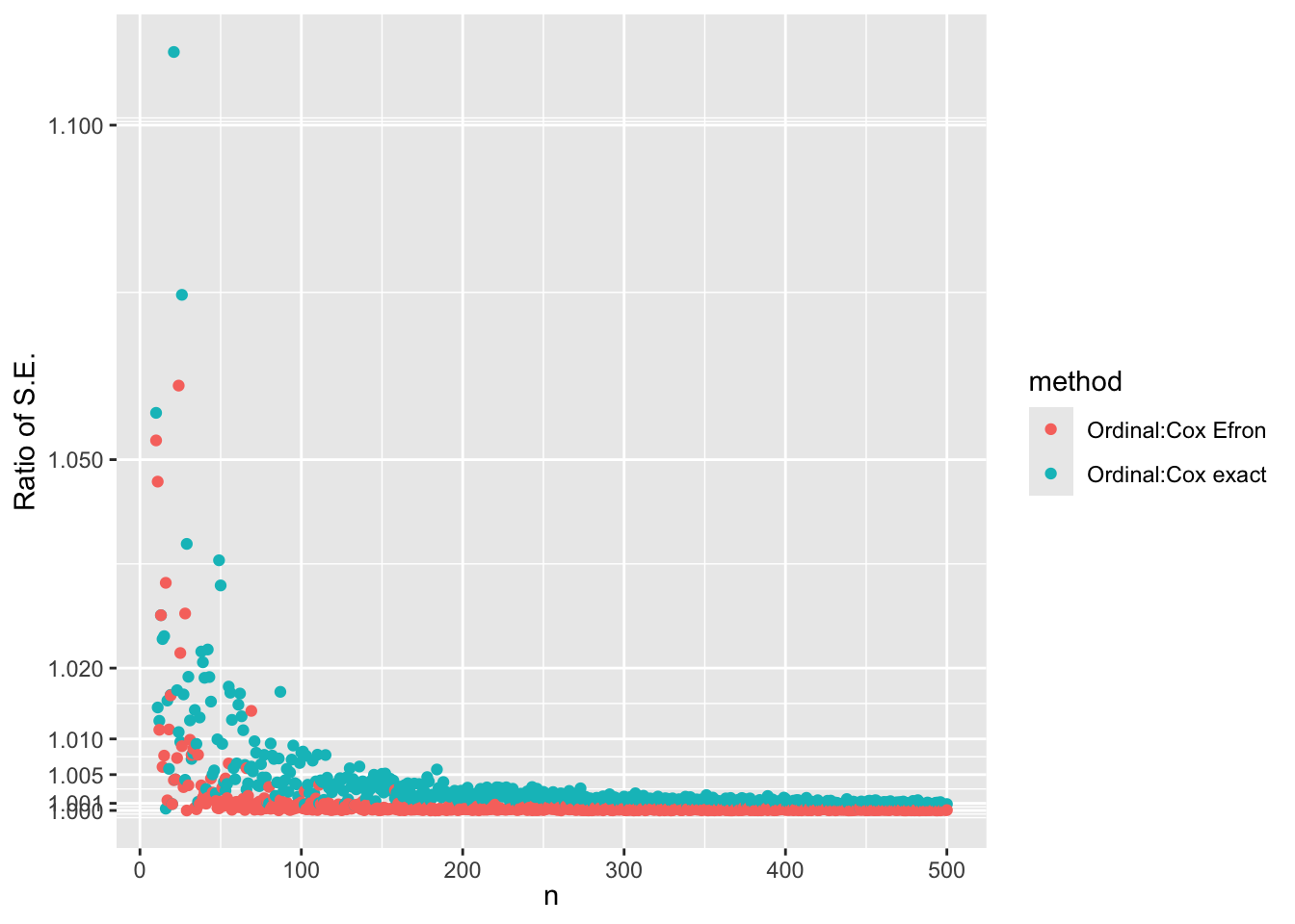
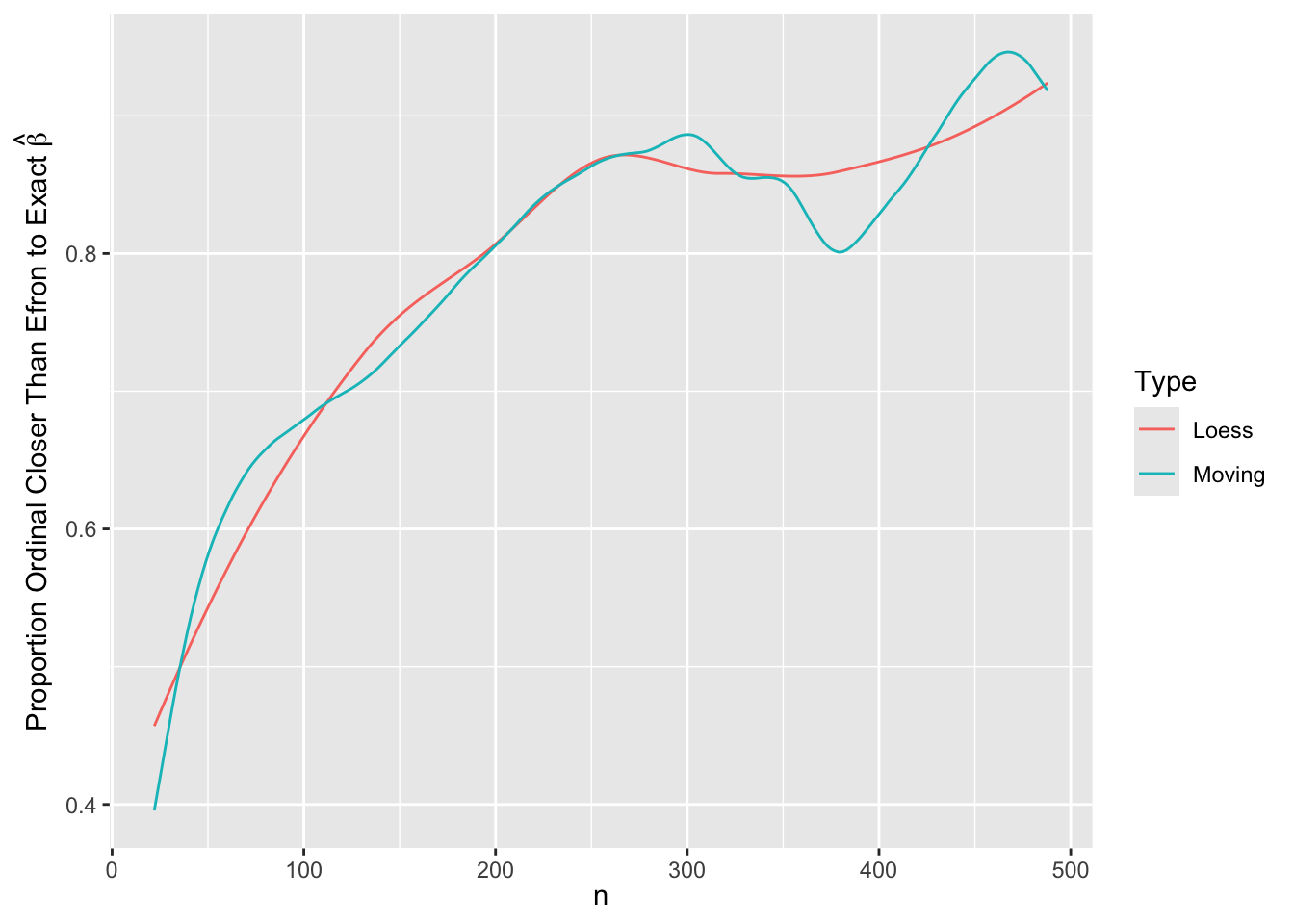
\(\hat{\beta}\) from the ordinal model is indistinguishable from \(\hat{\beta}\) from the exact likelihood Cox model for \(n > 80\). For lower \(n\) the differences are smaller than 0.3 standard errors of \(\hat{\beta}\). For estimating the standard error of \(\hat{\beta}\) the ordinal model agrees with the Efron approximation for \(n > 80\) but is also extremely close to the exact estimate. The median fold change margin of error against the exact Cox likelihood standard error is 1.0017009 over all \(n\).
25.4 The Continuum of Links
CPMs exist for an array of link functions representing distribution families, each link function giving rise to a different way that changes in covariate values change the distribution of Y. But the likelihood function used as an objective function against which to estimate intercepts \(\alpha\) and regression coefficients \(\beta\) has the same form for all links, and all links involve the same number of \(\alpha\) and \(\beta\). With CPMs with different links we find that
- When there are no covariates or \(\hat{\beta} = 0\), the estimated probabilities that \(Y\geq y\) or that \(Y=y\) are the same for all links.
- Thus the deviance (-2 log likelihood) for the null model (no \(\beta\)) is the same for all links.
This and all links having the same likelihood structure have important implications in favor of using the deviance, or equivalently the model likelihood ratio \(\chi^2\) statistic or AIC, for link selection. The rms Olinks function facilitates the calculations as shown in examples below. Compare this with trying to compare the deviance of a Cox PH model with that of a parametric accelerated failure time model.
Better fitting models (up to the point of overfitting) probably have sharper probability estimates, i.e., estimates further from 0.5. This rewards the deviance by making it smaller. Ill-fitting models tend to be conservative about \(\hat{\alpha}\) and \(\hat{\beta}\), leading to cell probability (likelihood probability elements) closer to 0.5 and hence worse AIC and pseudo \(R^2\).
For related research see FC Genter and VT Farewell 1985.
25.5 Effective Sample Sizes
Ordinal models give us a new opportunity to estimate effective sample size (ESS), i.e., the number of uncensored observations that has the same statistical information as our mixture of censored and uncensored observations. A new option lpe (“likelihood probability element”) to orm will cause orm.fit to save an \(N\)-vector of lpes in the fit object. These are the log-likelihoods contributed by each observation. By setting the ESS for all the uncensored observations to the number \(u\) of such observations, one can solve for a multiplier of -2 log likelihood that makes the scaled -2 LL of these \(u\) observations add up to \(u\). The multiplier is then used to scale the -2 LL for the censored observations to estimate their ESS.
The Cox model does not provide a per-observation ESS because the likelihood is computed only for risk sets not for individual observations.
25.6 The rms Package for Survival Analysis Using Ordinal Regression
Many general functions apply to all rms model fitting functions, e.g.
Function: generates an R function expressing the model’s linear predictorPredict: easy calculation of predicted value and confidence limitsnomogram: plots nomogramsanova: comprehensive ANOVA tablesummary: single-number effect estimatescontrast: general contrasts and profile likelihood confidence intervalsvalidate: resampling validation of model performance metricscalibrate: resampling overfitting-corrected calibration curvesintCalibration: newrms8.0 function for internal calibration plots for a series of cut-pointslatex: express the fitted model in mathematical form using \(\LaTeX\) markup
The rms orm function has been generalized in version 8.0 to handle general censoring patterns, and there are several new rms functions that use orm fits to produce output that is especially suited for survival analysis:
Ocens: packages survival and censoring times into a two-column matrixOcens2ord: convertsOcensobjects to discrete ordinal codes- Makes adjustments for left, right, interval censoring
- Each observation must be associated with one or two ordinal model intercepts
- Censored observations must use existing intercept parameters that are defined by distinct uncensored values
- E.g. an observation right-censored at 4 years considers the point to be right-censored at 3.9 years if the last uncensored value before 4y was 3.9
- Observations censored after the last uncensored time point are very informative and cause creation of a new final uncensored category at the lowest of such censoring times (or, in the rare case that this value ties exactly with the last uncensored time, one grid unit above it, to keep the category distinct)
- Interval-censored observations create Turnbull intervals and are given a lot of attention by
Ocensso that unique likelihood contributions result - The nonparametric survival curve estimates are saved so that the link function of them can be used as started values for MLE, with starting values for \(\beta\) equal to zero
survest: estimate survival probabilities and confidence intervals for subjects described in a data framesurvplot: plot survival curves and confidence bands for easily-specified covariate combinationsSurvival: generate an R function that computes survival probabilities and confidence limitsMean: generate an R function that computes restricted mean survival time and confidence limitsplotIntercepts: plot intercepts vs. corresponding \(y\)-values, with optional log scale for \(y\); linearity of such plots would indicate that \(y\) was correctly transformed for the corresponding parametric modelordParallel: estimate the effects of covariates over time- Re-fits the ordinal model using a sequence of cutoffs to check the adequacy of the link function, i.e., to check parallelism of link-transformed survival curves
ordESS: computes the effective sample size in the presence of general censoring, and plots per-observation ESS against censoring time (e.g., interval-censored observations with narrower intervals will convey more information)residuals.orm:type='score'creates a score matrix that respects general censoring; this is used byrobcovto get robust sandwich covariance estimates
The Hazard function generator is not available for ordinal models. Discrete hazard functions are not very useful for continuous failure times.
In addition to the survival-specific functions there is a new general function in rms just for orm fits: Olinks. See examples below.
25.6.1 Rank Discrimination Indexes Computed by orm
For uncensored data, orm computes Spearman’s \(\rho\) rank correlation between predicted and observed Y. There is no version of \(\rho\) for censored data. Somers’ \(D_{xy}\) has been added to orm because this works for both uncensored and censored data. \(D_{xy}\) is \(2\times (c - \frac{1}{2})\) where \(c\) is the generalized \(c\)-index or concordance probability, computed extremely quickly by Therneau’s survival package concordancefit function.
25.7 Goodness of Fit Overview
Ordinal semiparametric CPM models —
- Essentially are covariate-shifted empirical cumulative distribution function estimators
- Usual \(X\)-assumptions related to how many d.f./parameters specified (linearity, additivity)
- Intercepts move around as needed to fit any shape of distribution for a specific \(X\)
- \(\rightarrow\) no ordinary distributional assumption to check
- Assumes how shape of \(Y\) distribution varies across levels of \(X\)
- link-transformed \(P(Y \geq y | X)\) as a function of \(y\) are parallel
25.7.1 Quantitative GOF Assessments
- Embed the model in a more general model with more parameters
- use AIC to judge which of the two models is more likely to have better cross-validated accuracy
- examples of more general models: partial proportional odds model, polytomous (multinomial) logistic regression
- example
- this is the preferred method but is not covered in this chapter although it is related to the \(y\)-varying \(\beta\) plots to follow
- future addition to the
rmsormfunction will make this easier
- Compare deviances (-2 log likelihood) for different links using the same \(X\) design
- equivalent to judging model likelihood ratio \(\chi^2\), AIC, and pseudo \(R^2\)
- easy to do with
rmsOlinksfunction (new in 8.0) - several examples follow
25.7.2 Qualitative/Graphical GOF Assessments
- Stratify by a key predictor or by predicted values from a tentative model, and for each stratum compute a nonparametric cumulative distribution estimate (ECDF or Kaplan-Meier), link-transform it, and assess parallelism
- For a series of \(y\) cutoffs fit binary models for the event occurrence \(Y \geq y\) and plot the estimated \(\beta\) against \(y\), and add a smoother
- Examples also given with formal tests of \(X\times y\) interaction using GEE
- With censored \(Y\), some binary indicators of \(Y\geq y\) cannot be determined and these observations are omitted
- The same as the previous dichotomization approach but on the overall linear predictor, seeing how its slope varies away from 1.0 over the set of cut-points
- This may be better than stratifying by a linear predictor and getting stratified Kaplan-Meier estimates
- Internal calibration plots: plot predicted \(P(Y \geq y)\) vs. observed smoothed proportions (smoothed moving overlapping windows of Kaplan-Meier estimates or using an adaptive flexible hazard model -
hareKooperberg et al. (1995), Kooperberg & Clarkson (1997)) - Similar to the previous method but plot both predicted and observed probabilities against a covariate (overlapping window moving averages)
- Shepherd et al. (2016) probability-scaled residual plot (like linear model Q-Q plot but check against a uniform distribution); extended to censored data here
25.7.3 Sample Size Limitations
- Just as when estimating parameters, the effective sample size limits the information content in goodness-of-fit diagnostics (informal or formal)
- \(N\) needed for relative comparisons that do not involve intercept \(\alpha\) have their own sample size requirements to achieve a given power or precision
- Absolute estimates that involve \(\alpha\) and GOF assessments related to distribution shifts need sufficient \(N\) to be able to estimate entire distributions
- RMS Chapter 20: need 184 uncensored observations to estimate entire cumulative distribution within margin of error \(\pm 0.1\) with probability \(\geq 0.95\)
- For margin of error \(\pm 0.05\), sample size required is \(4\times\) higher at 736
So in non-huge datasets some GOF assessments are noisy and hard to use for decision making.
NoteSample Size Requirements for Discriminating Links Using Deviance
What sample sizes are needed for deviances from various links to be able to discern the correct link? Let’s simulate multiple datasets with varying \(N\), with no censoring, replicating each \(N\) 50 times and averaging the 50 deviances. Data are generated using a logit link. The deviance from the ideal logit link is subtracted from each non-logit link’s deviance.
Code
sim <- function(n) {
  age <- rnorm(n, 50, 12)
  sex <- sample(c('male', 'female'), n, TRUE)
  ran <- rnorm(n)
  lp  <- 0.04 * (age - 50) + 0.8 * (sex == 'female')
  y   <- exp(0.5 + lp + rlogis(n) / 3)
  f   <- orm(y ~ age + sex + ran, x=TRUE, y=TRUE)
  # One cloglog fit would not converge; fixed by gradtol
  Olinks(f, dec=5, gradtol=0.01)[c('link', 'deviance')]
}
R <- expand.grid(n = c(20, 40, 60, 80, 100, 150, 200, 300, 400, 500),
                 i = 1:50)
setDT(R)   # Change R to a data.table
set.seed(8)
w <- R[, sim(n), by=.(n, i)]
# For each run, subtract logit deviance from others
g <- function(dev, link) {
  j <- link == 'logistic'
  list(link=link[! j], dif=dev[! j] - dev[j])
}
u <- w[, g(deviance, link), by=.(n, i)]
m <- u[, .(dif = mean(dif)), by=.(link, n)]
ggplot(m, aes(x=n, y=dif, col=link)) + geom_line() +
  xlab(expression(N)) + ylab('Deviance Minus logit Deviance') +
  geom_hline(yintercept=3.84, alpha=0.4)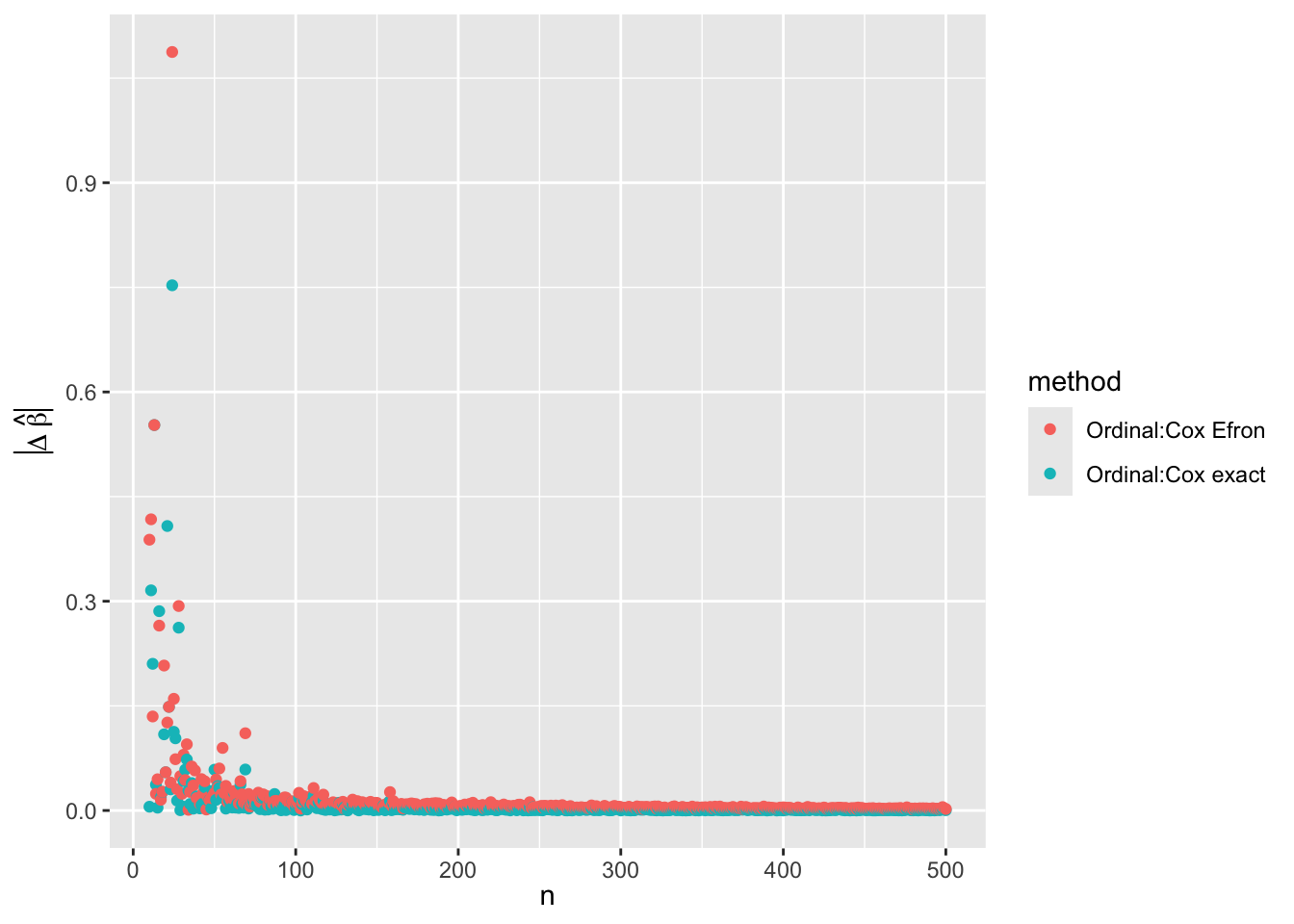
A reference line is drawn at the \(\chi^{2}_{1}\) 0.95 critical value of 3.84 to give a rough idea of a noise reference level. Distinguishing between the logit and probit links requires \(N > 250\) whereas the log-log and complementary log-link links are distinguishable from the logit link by \(N=60\).
But these are on the average. There is a lot of sample-to-sample variability in deviances and deviance orderings. Instead of showing mean differences, plot the 0.1 quantiles of differences within each 50-run batch.
Code
lo <- u[, .(dif = quantile(dif, 0.1)), by=.(link, n)]
ggplot(lo, aes(x=n, y=dif, col=link)) + geom_line() +
  xlab(expression(N)) + ylab('Deviance Minus logit Deviance') +
  geom_hline(yintercept=3.84, alpha=0.4)
Another way: plot the proportion of times that the logit deviance was the smallest of the four, and the proportion of times that either the logit or probit was the smallest.
Code
g <- function(dev, link) {
  j <- which.min(dev)
  k <- link %in% c('logistic', 'probit')
  list(glink   = c('logit', 'logit or probit'),
       correct = c(link[j] == 'logistic',
                   min(dev[k]) < min(dev[! k]) ) )
}
cr <-  w[, g(deviance, link), by=.(n, i)]
m  <- cr[, .(prop = mean(correct)), by=.(n, glink)]
ggplot(m, aes(x=n, y=prop, col=glink)) + geom_line() +
  xlab(expression(N)) + ylab('Proportion Correct') +
  guides(color=guide_legend(title='')) +
  geom_hline(yintercept=0.9, alpha=0.3)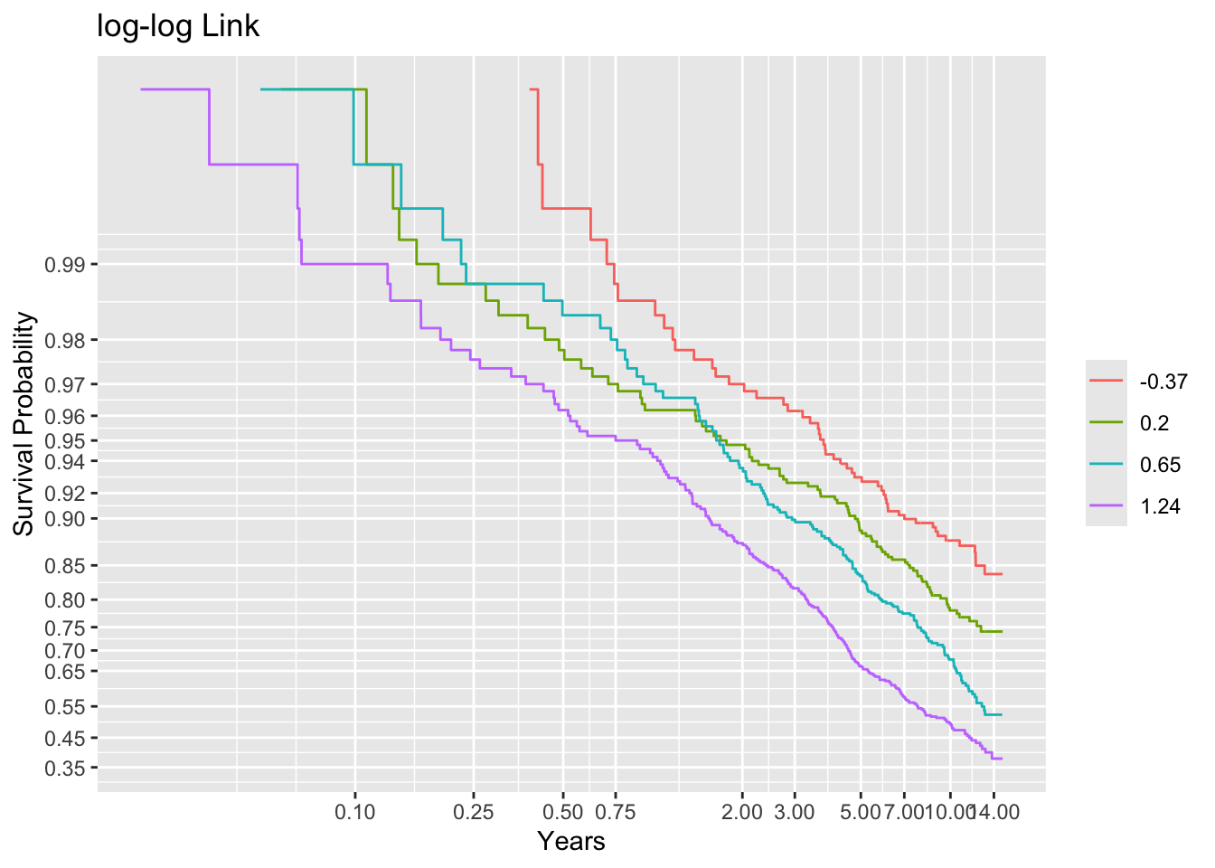
To have \(> 0.9\) chance that the link with the minimum deviance is the correct or very similar link, we need \(N > 125\). To have confidence that it is the logit link we need \(N > 300\).
25.7.4 Overall Recommendations and Strategy
%%{init: {'theme':'forest'}}%%
mindmap
  root(Strategy for Link Specification)
    Pre-specification
      Choose link that well-fitted a similar dataset
      Subject matter knowledge
        Chronic process, constant X effects over time
          PH model; log-log link
        Acute process, front-loaded X effects
          Accelerated failure time; logit link
    Controlled flexibility
      Compare deviances of logit, log-log, c-log-log links
      Check flatness of overall linear predictor effect over y cutpoints
      Predictor of special importance: check flatness of its partial effect over y cutpoints
- Link function is a bit less important than it seems
- Impact of link can be lost in the noise of estimating \(\beta\) especially when \(N\) is not large
- Semiparametric models shift intercept spacings as needed so that for a given \(X\) there is no distributional assumption for \(Y\)
- Ordinal model analyses are unaffected by transformation of \(Y\) until one computes \(E(Y | X)\)
- By contrast, compare accuracy of \(\hat{S}(t | X)\) for different links with accuracy of accelerated failure time parametric \(S(t | X)\) estimates for different \(Y\)-transformations
- Impact of the link on interpretation is perhaps larger than impact on estimating probabilities and quantiles
- Odds ratios with logit link, hazard ratios with log-log link
- But if one emphasizes covariate-specific differences in survival curves, interpretation is easier and perhaps more robust
Suggested Strategy
Remember that the \(X\) effects need to be carefully specified as with all regression models. An ordinal model link function specifies the transformation of cumulative probabilities of \(Y\) such that for different \(X\) the cumulative distributions are parallel. Ideally the link function should not necessitate \(y\)-dependent covariate effects, i.e., allows us to act as if effects of covariates are constant over time for the chosen distribution family.
- If you want to have a completely pre-specified statistical analysis plan, use subject matter knowledge to reason whether predictor effects are likely to have constant effects on instantaneous risk, or they have front-loaded effects that wane with time
- Use log-log link (assumes constant hazard ratios) for the first
- Use logit link for the second (accelerated failure time model)
- Don’t use the probit link
- Very similar to logit link but has no easy interpretation of effect estimates
- Only use it when you think that normality of residuals is in play after some \(Y\)-transformation and you want to guarantee efficiency of semiparametric estimates with respect to parametric counterparts
- Entertain 3 links that are very different from each other
- logit, log-log, and complementary log-log
- If previous analyses on similar data indicate a good fit of one of the links, pre-specify use of that one
- Develop a tentative model by carefully specifying predictors, non-linearities, and interactions
- Compare deviances of the three models (using e.g.
rms::Olinks) and note the link with the smallest (best) deviance - Compute the linear predictor \(X\hat{\beta}\) from each of the three fits
- Re-fit a series of binary models over \(y\) cuts, using each link
- Plot the coefficient of \(X\hat{\beta}\) over cuts (the coefficients must have a weighted average of 1.0)
- These steps are automated by
rms::ordParallel(fit, lp=TRUE) - Select the link that has the best trade-off of deviance and flatness in these plots
- If there is a pre-specified predictor of major importance to interpretation (e.g., treatment), see how \(\beta\) for that predictor varies over \(y\)-cuts
rms::ordParallel(fit, which=...)- Choose a link that makes that predictor fit well subject to overall fit not being severely affected
25.8 Simple Examples With Goodness of Fit Assessments
- Simulate survival times from two models
- Exponential distribution with proportional hazards (PH) for the covariate effects
- covariate effects are constant over time on the hazard ratio scale
- the AFT class and PH intersect for exponential and Weibull models when covariate effects operate multiplicatively on the hazard
- \(T\) has an AFT model (e.g., \(\log(T)\) has a normal, logistic distribution)
- An accelerated failure time model – additive covariate effects with logistic distribution residuals
- covariates have decreasing effects over time on hazard ratios
- For each simulated dataset fit the right model and a wrong model
- Run model diagnostics
ordParallelto check parallelism assumption / link adequacy- Note that neither Cox-Snell residual plots nor smoothed score residual plots are sensitive to lack of fit in this setting; smoothed score residual plots (Schoenfeld residuals) only work for the Cox model
- Model fits as labeled as follows (
x11andx22are correct models)- f11: exponential data with PH fitted with Cox PH
- g11: exponential data with PH fitted with log-log family ordinal model
- g12: exponential data with PH fitted with logistic family AFT ordinal model
- f21: logistic distribution data with non-PH fitted with the Cox model
- g21: logistic distribution data fitted with log-log ordinal model
- g22: logistic distribution data fitted with logistic AFT ordinal model
- Censoring distribution is \(U(2, 15)\) and only right censoring is present
Code
require(rms)
require(survival)
require(ggplot2)    # needed for labs(title=...) etc.
n <- 2000
set.seed(2)
cens <- runif(n, 2, 15)
age  <- rnorm(n, 50, 12)
label(age) <- 'Age'
units(age) <- 'year'
sex  <- sample(c('male', 'female'), n, TRUE)
ran  <- rnorm(n)   # irrelevant random covariate
# Exponential model with PH
lp   <- 0.04 * (age - 50) + 0.8 * (sex == 'female')
label(lp) <- ''
h    <- 0.02 * exp(lp)      # hazard function
t1   <- -log(runif(n))/h    # simulated failure times
e1   <- t1 <= cens
sum(e1)              # uncensored obs
[1] 501Code
y1   <- pmin(t1, cens)
units(y1) <- 'year'
S1   <- survival::Surv(y1,  e1)
Y1   <- Ocens(y1, ifelse(e1, y1, Inf))
l    <- 13:15
cbind(t1, cens)[l, ]
t1 cens
[1,] 15.713940 11.886673
[2,] 2.666562 4.350661
[3,] 86.924433 7.268668Code
S1[l, ][1] 11.886673+ 2.666562 7.268668+Code
Y1[l, ][1] 11.88667+ 2.66656 7.26867+Code
# Right-censored values beyond the last uncensored time are very
# informative, and for them Ocens2ord (called internally by orm) creates
# a final uncensored level at the minimum of such censoring times (or,
# if that value ties exactly with the last uncensored time, one grid
# unit above it, to keep the category distinct)
max.uncens <- max(t1[e1])
min.cens.after.last.uncens <- min(t1[! e1 & (t1 > max.uncens)])
c(max.uncens, min.cens.after.last.uncens)
[1] 13.78902 13.88974Code
a <- S1[,1]
b <- S1[,2]
max(a[b == 1])
[1] 13.78902Code
min(a[b == 0 & a > max.uncens])[1] 13.79099Code
m <- which(a == min(a[a > max.uncens & b == 0]))
S1[m, ]
[1] 13.79099+Code
Y1[m,, drop=FALSE ][1] 13.79099+Code
l <- 13:15
S1[l, ]
[1] 11.886673+ 2.666562 7.268668+Code
Y1[l, ][1] 11.88667+ 2.66656 7.26867+Code
# Logistic AFT model
t2   <- exp(0.5 + lp + rlogis(n) / 3)
e2   <- t2 <= cens
sum(e2)
[1] 1697Code
y2   <- pmin(t2, cens)
units(y2) <- 'year'
S2   <- survival::Surv(y2, e2)
Y2   <- Ocens(y2, ifelse(e2, y2, Inf))
t1 <- round(t1, 2)
t2 <- round(t2, 2)
dd <- datadist(age, sex, ran); options(datadist='dd')
First see if we can discern the correct link functions if we knew the true linear predictor. Stratify this linear predictor into groups each containing 500 subjects, compute Kaplan-Meier estimates stratified by this, and plot the results with 3 transformations of the y-axis, looking at parallelism.
Code
g <- round(cutGn(lp, 500), 2)
# Compute the number of events per lp group
table(t1 <= cens, g)
g
-0.37 0.2 0.65 1.24
FALSE 448 415 356 280
TRUE 52 85 144 220Code
f <- npsurv(S1 ~ g)
ggplot(f, trans='loglog', logt=TRUE, conf='none') + labs(title='log-log Link')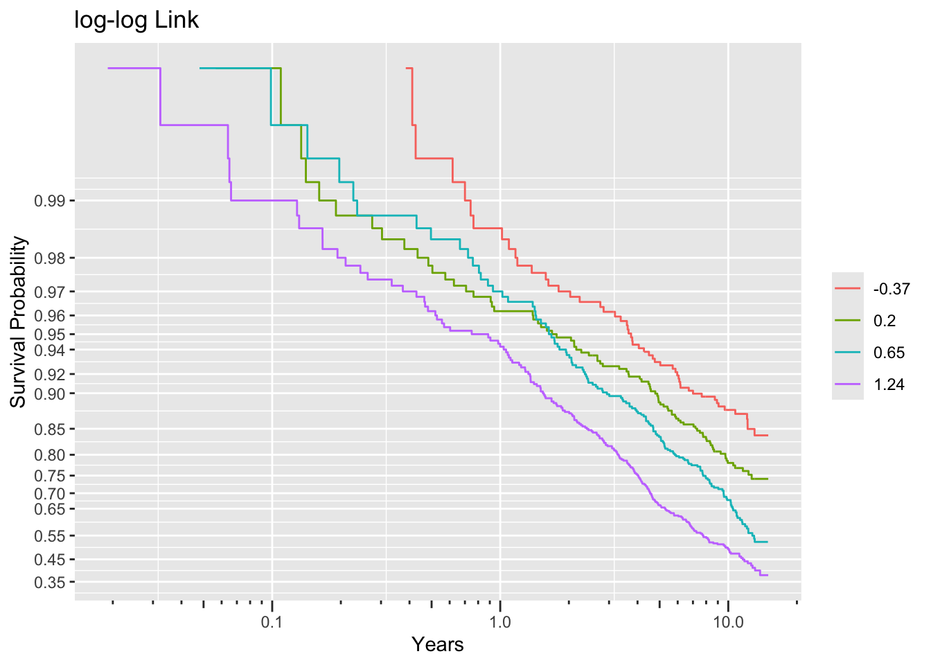
Code
ggplot(f, trans='logit', logt=TRUE, conf='none') + labs(title='logit Link')
Code
ggplot(f, trans='probit', logt=TRUE, conf='none') + labs(title='probit link')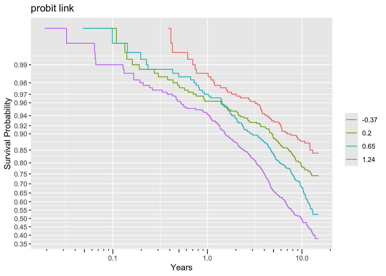
Non-parallelism (inadequacy of the link function) is best judged by comparing vertical distance between the outer transformed survival curves. The probit link clearly does not work, but the logit link and the perfect-fitting log-log link are surprisingly close. This is perhaps related to the simplicity of the first simulation model.
Let’s fit a series of models to examine fitted linear predictors from the log-log and logit model. mscore=TRUE computes the \(n\times p\) score matrix correctly if censoring is present.
Code
f11  <- cph(S1 ~ age + sex + ran, surv=TRUE, x=TRUE, y=TRUE)
g11  <- orm(Y1 ~ age + sex + ran, family='loglog',   mscore=TRUE, x=TRUE, y=TRUE)
g12  <- orm(Y1 ~ age + sex + ran, family='logistic', mscore=TRUE, x=TRUE, y=TRUE)
f21  <- cph(S2 ~ age + sex + ran, surv=TRUE, x=TRUE, y=TRUE)
g21  <- orm(Y2 ~ age + sex + ran, family='loglog',   mscore=TRUE, x=TRUE, y=TRUE)
g22  <- orm(Y2 ~ age + sex + ran, family='logistic', mscore=TRUE, x=TRUE, y=TRUE)
25.8.1 Data Simulated from Exponential Distribution with PH
Compare the models fitted on exponential-distributed survival times in various ways, and check whether better-fitting models have robust standard errors of \(\hat{\beta}\) that is closer to the usual standard errors than less-well-fitting models. Show
- model
printoutput - comparison \(\hat{\beta}\) across models
- correlation matrix of linear predictors \(X\hat{\beta}\) across models
- usual vs. robust sandwich standard errors
Code
# Compare betas first
cbetas <- function(fits) {
  nam <- names(fits)
  u <- function(f) {
    k <- num.intercepts(f)
    if(k == 0) coef(f) else coef(f)[-(1 : k)]
  }
  cat('betas:\n\n')
  print(sapply(fits, u))
  # Compute correlation matrix of linear predictors
  cat('\nCorrelations of linear predictors:\n\n')
  print(round(cor(sapply(fits, function(x) x$linear.predictors)), 5))

  # Compute SEs from information matrix and from sandwich estimator
  u <- function(f, nam) {
    k <- num.intercepts(f)
    se1 <- if(k == 0) sqrt(diag(vcov(f)))
            else sqrt(diag(vcov(f, intercepts='none')))
    se2 <- if(k == 0) sqrt(diag(vcov(robcov(f))))
            else sqrt(diag(vcov(robcov(f), intercepts='none')))
    cat('\n', nam,
        ': standard errors from information matrix and robust sandwich estimator\n\n',
        sep='')
    print(round(rbind(Info = se1, Robust=se2), 4))
    cat('\n')
  }
  w <- sapply(names(fits), function(nm) u(fits[[nm]], nm))
  invisible()
}
Code
fits <- list(Cox=f11, loglog=g11, logit=g12)
maketabs(fits)
Cox Proportional Hazards Model
cph(formula = S1 ~ age + sex + ran, x = TRUE, y = TRUE, surv = TRUE)
| Model Tests | Discrimination Indexes |
|
|---|---|---|
| Obs 2000 | LR χ2 203.54 | R2 0.100 |
| Events 501 | d.f. 3 | R23,2000 0.095 |
| Center 1.6525 | Pr(>χ2) 0.0000 | R23,501 0.330 |
| Score χ2 200.15 | Dxy 0.346 | |
| Pr(>χ2) 0.0000 |
| β | S.E. | Wald Z | Pr(>|Z|) | |
|---|---|---|---|---|
| age | 0.0413 | 0.0039 | 10.62 | <0.0001 |
| sex=male | -0.8839 | 0.0960 | -9.21 | <0.0001 |
| ran | 0.0231 | 0.0454 | 0.51 | 0.6119 |
-log-log Ordinal Regression Model
orm(formula = Y1 ~ age + sex + ran, family = "loglog", x = TRUE,
    y = TRUE, mscore = TRUE)
| Model Likelihood Ratio Test |
Discrimination Indexes |
Rank Discrim. Indexes |
|
|---|---|---|---|
| Obs 2000 | LR χ2 203.78 | R2 0.099 | Dxy 0.346 |
| ESS 547.4 | d.f. 3 | R23,2000 0.096 | |
| Censored R=1499 | Pr(>χ2) <0.0001 | R23,547.4 0.307 | |
| Distinct Y 502 | Score χ2 200.38 | |Pr(Y ≥ median)-½| 0.370 | |
| Y0.5 4.052121 | Pr(>χ2) <0.0001 | ||
| max |∂log L/∂β| 2×10⁻¹⁰ |
| β | S.E. | Wald Z | Pr(>|Z|) | |
|---|---|---|---|---|
| age | -0.0414 | 0.0039 | -10.62 | <0.0001 |
| sex=male | 0.8846 | 0.0960 | 9.21 | <0.0001 |
| ran | -0.0231 | 0.0454 | -0.51 | 0.6111 |
Logistic (Proportional Odds) Ordinal Regression Model
orm(formula = Y1 ~ age + sex + ran, family = "logistic", x = TRUE,
    y = TRUE, mscore = TRUE)
| Model Likelihood Ratio Test |
Discrimination Indexes |
Rank Discrim. Indexes |
|
|---|---|---|---|
| Obs 2000 | LR χ2 195.75 | R2 0.095 | Dxy 0.347 |
| ESS 546.7 | d.f. 3 | R23,2000 0.092 | |
| Censored R=1499 | Pr(>χ2) <0.0001 | R23,546.7 0.297 | |
| Distinct Y 502 | Score χ2 189.52 | |Pr(Y ≥ median)-½| 0.372 | |
| Y0.5 4.052121 | Pr(>χ2) <0.0001 | ||
| max |∂log L/∂β| 4×10⁻¹⁰ |
| β | S.E. | Wald Z | Pr(>|Z|) | |
|---|---|---|---|---|
| age | -0.0473 | 0.0047 | -10.11 | <0.0001 |
| sex=male | 1.0272 | 0.1122 | 9.15 | <0.0001 |
| ran | -0.0223 | 0.0549 | -0.41 | 0.6845 |
Code
cbetas(fits)betas:
Cox loglog logit
age 0.04132661 -0.04135691 -0.04729157
sex=male -0.88385827 0.88464058 1.02719281
ran 0.02305826 -0.02310765 -0.02229077
Correlations of linear predictors:
Cox loglog logit
Cox 1.00000 -1.00000 -0.99996
loglog -1.00000 1.00000 0.99996
logit -0.99996 0.99996 1.00000
Cox: standard errors from information matrix and robust sandwich estimator
age sex=male ran
Info 0.0039 0.0960 0.0454
Robust 0.0040 0.0956 0.0439
loglog: standard errors from information matrix and robust sandwich estimator
age sex=male ran
Info 0.0039 0.0960 0.0454
Robust 0.0040 0.0957 0.0439
logit: standard errors from information matrix and robust sandwich estimator
age sex=male ran
Info 0.0047 0.1122 0.0549
Robust 0.0048 0.1122 0.0526So the model choice is not very relevant for getting estimates on the linear scale as judged by the correlations between \(X\hat{\beta}\) all being near 1.0 in absolute value.
Plot effects of predictors over time to check link functions (parallelism assumption).
Code
czph <- function(fit) {
  z <- cox.zph(fit)
  cat('cox.zph tests for proportional hazards\n\n')
  print(z)
  spar(mfrow=c(2,2))
  plot(z, resid=FALSE)
}
czph(f11)
cox.zph tests for proportional hazards
chisq df p
age 1.29500 1 0.26
sex 0.41149 1 0.52
ran 0.00267 1 0.96
GLOBAL 1.73541 3 0.63
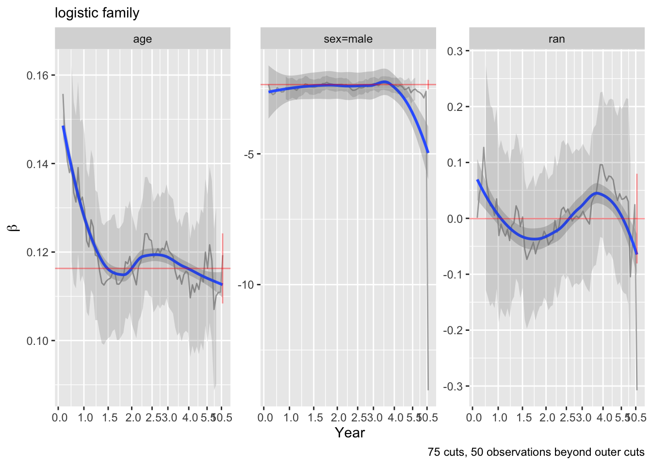
Code
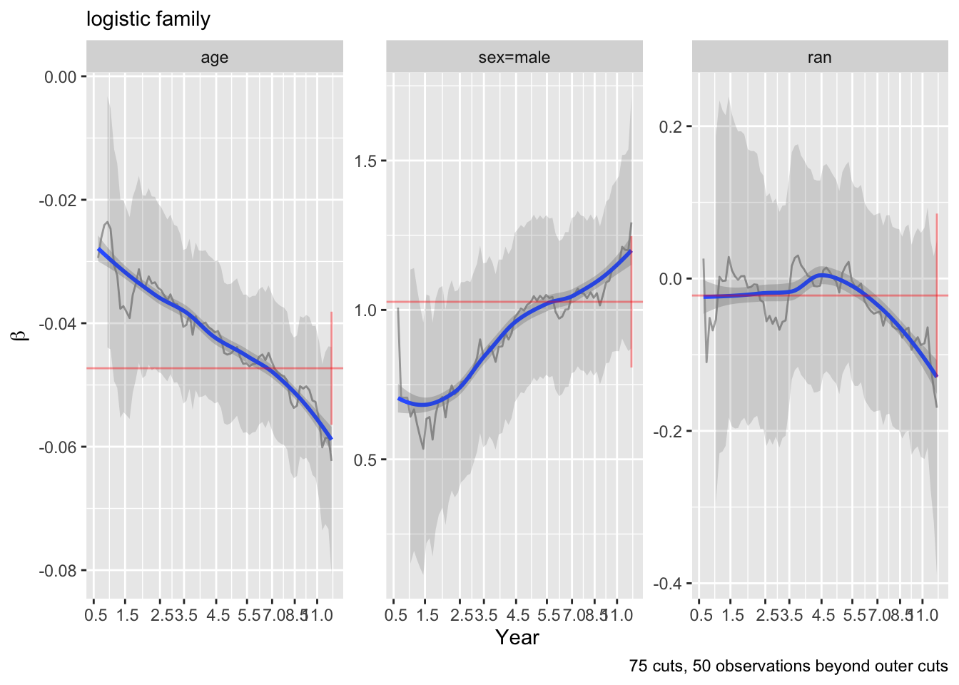
ordParallel(g11)
ordParallel(g12)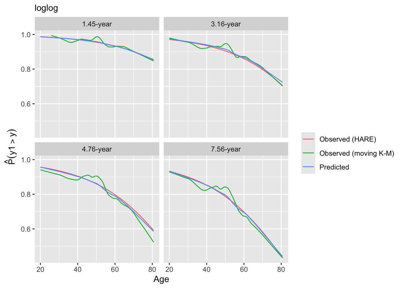
- Cox model: Schoenfeld residual plots appear to be flat, and low \(\chi^2\) statistics for testing PH
- log-log link ordinal model: flat effects over time to within the limits of the confidence bands show our limits of estimating time-specific effects
- logit link: systematic changing of effects over time with meaningful changes in \(\hat{\beta}\) for the two relevant variables, indicating time-dependent covariate effects / non-parallelism of logit of \(S(t | X)\)
Consider the estimated linear predictor to be a single summary predictor. Refit models with just that one predictor and plot its coefficient over the cuts.
Code
ordParallel(g11, lp=TRUE)
ordParallel(g12, lp=TRUE)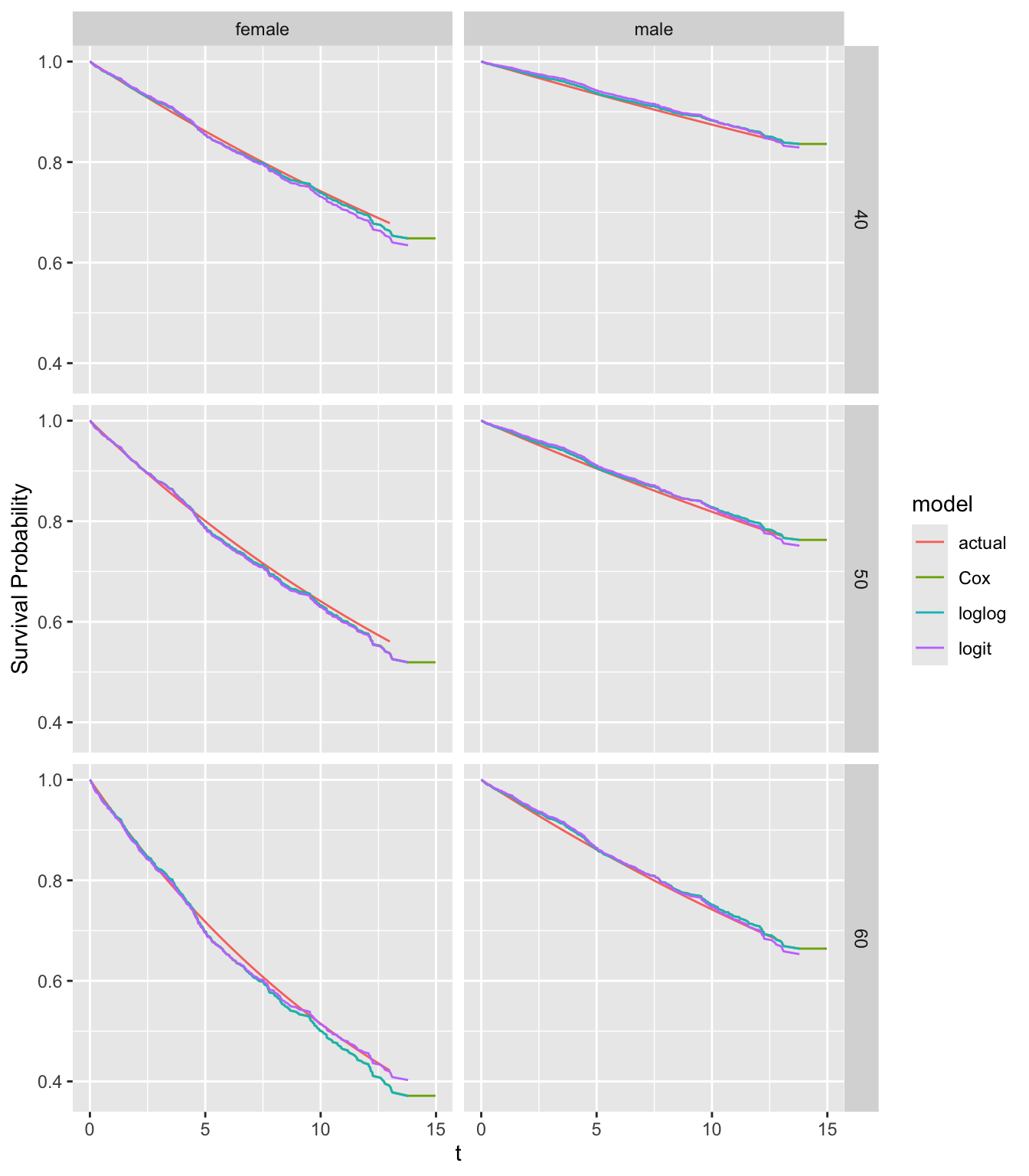
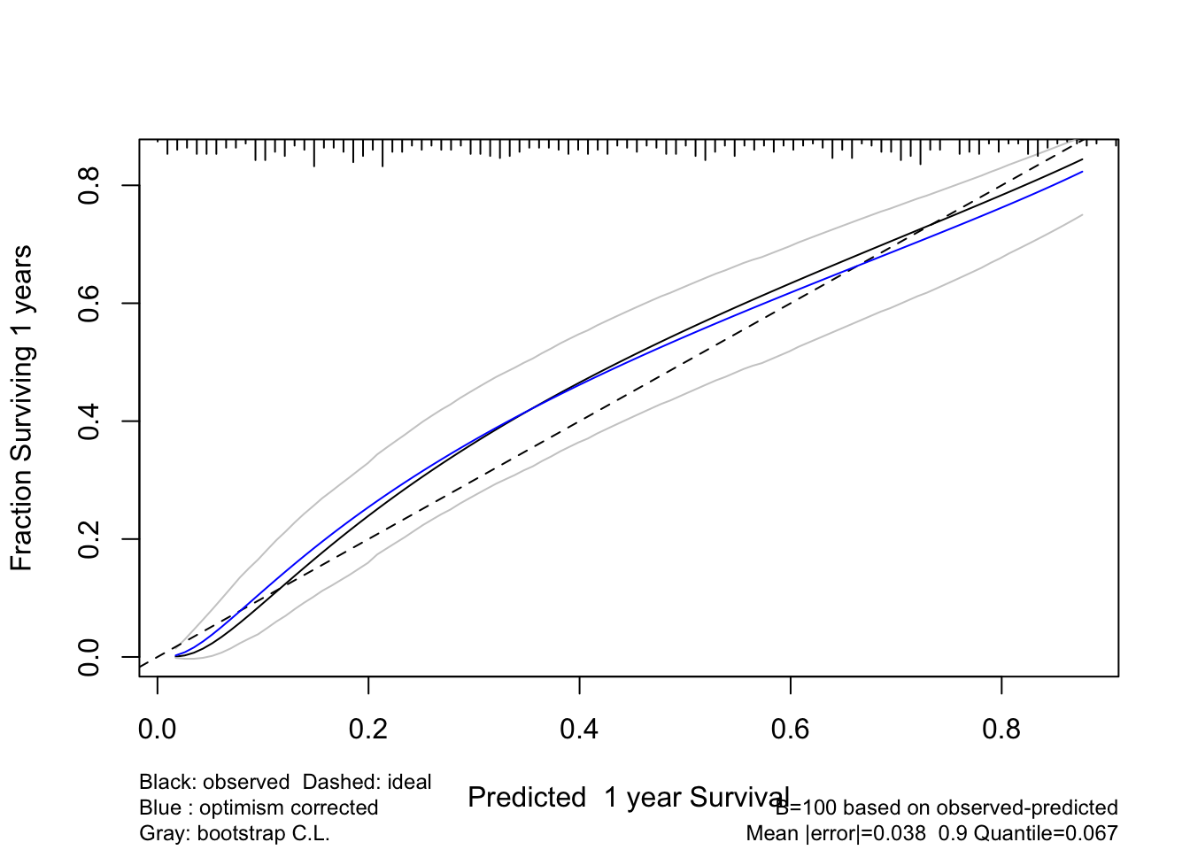
Look at internal calibration-in-the-small curves and also print statistics for calibration-in-the-large. Cut-points are chosen so that there are 100 uncensored observations between cut-points and beyond outer cut-points. Here the relationship between predicted and observed survival probabilities is estimated using three methods: moving Kaplan-Meier estimates, hazard regression with polspline::hare, and adaptive ordinal models.
Code
intCalibration(g11, m=100, dec=2) + labs(subtitle=g11$family)
Calibration-in-the-large:

    y Mean Predicted P(Y > y) Observed P(Y > y)
 1.45                  0.9501            0.9500
 3.16                  0.8996            0.8991
 4.76                  0.8400            0.8391
 7.56                  0.7664            0.7653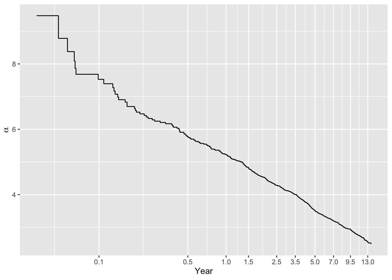
Code
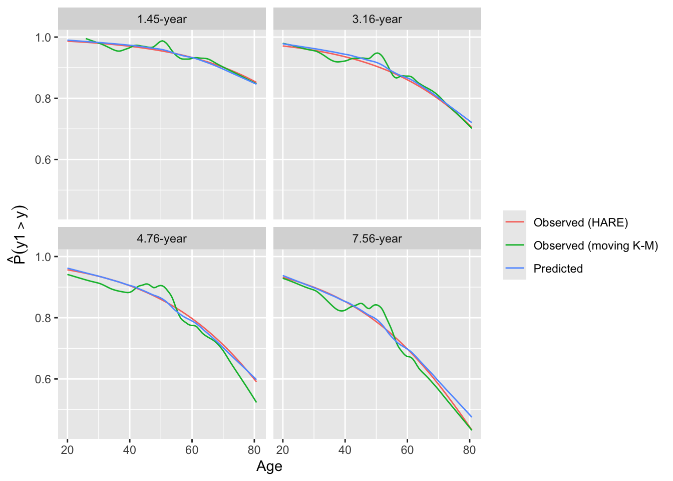
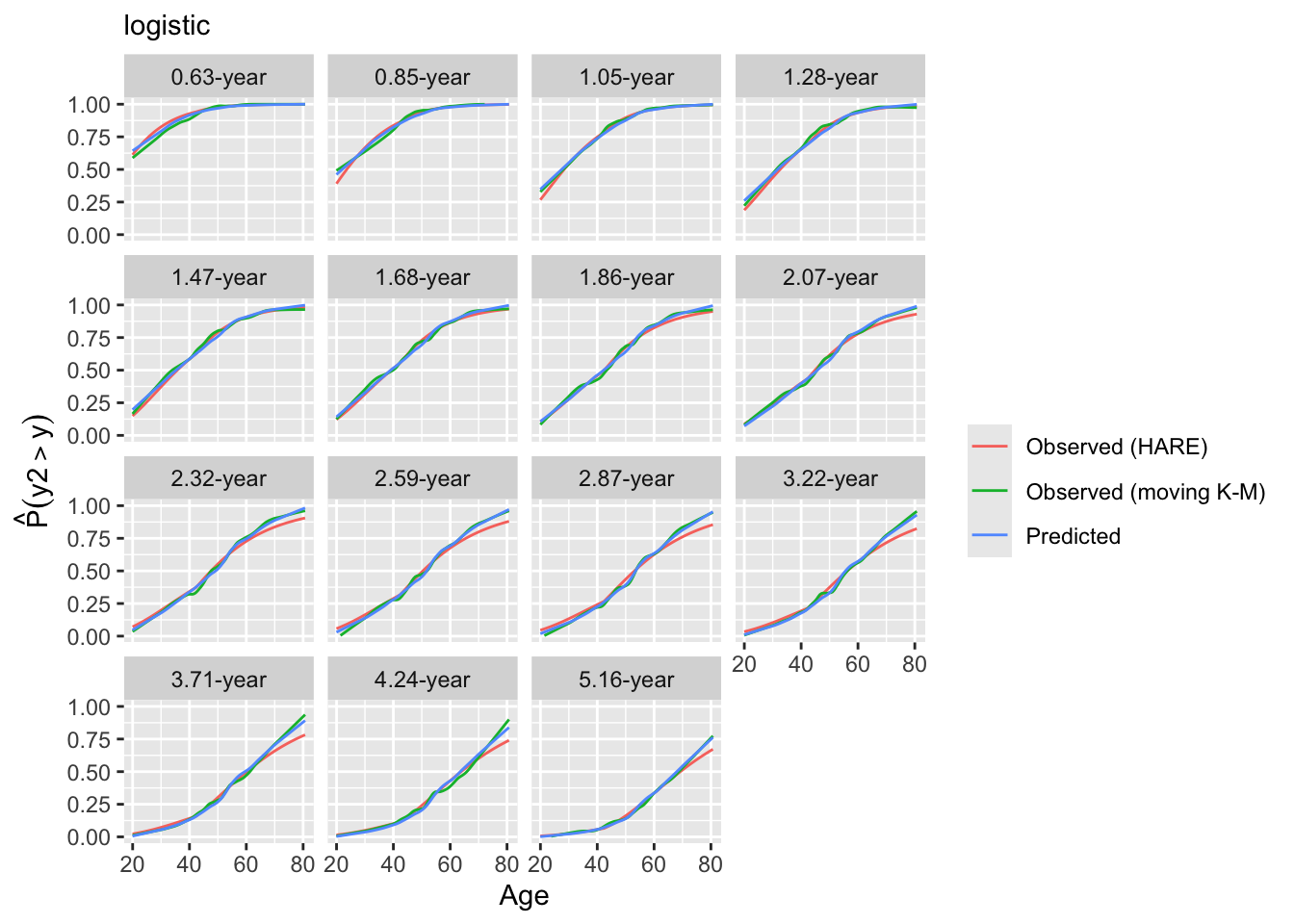
intCalibration(g12, m=100, dec=2) + labs(subtitle=g12$family)
Calibration-in-the-large:

    y Mean Predicted P(Y > y) Observed P(Y > y)
 1.45                  0.9505            0.9500
 3.16                  0.9009            0.8991
 4.76                  0.8421            0.8391
 7.56                  0.7689            0.7653
We can also check calibration with respect to a key predictor.
Code
intCalibration(g11, m=100, x=age, hare=FALSE, dec=2) +
  labs(subtitle=g11$family)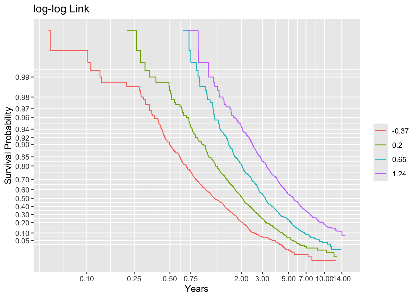
Code
intCalibration(g12, m=100, x=age, hare=FALSE, dec=2) +
  labs(subtitle=g12$fam)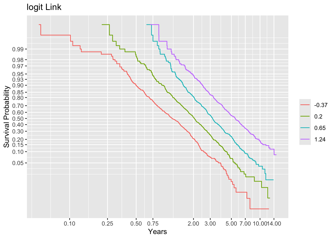
Let’s see if comparison of links based on log-likelihood measures gives us the same impression about the orm models.
Code
Olinks(g11) link null.deviance deviance AIC LR R2
1 loglog 8141.307 7937.530 8945.530 203.776 0.307
2 logistic 8141.307 7945.554 8953.554 195.752 0.297
3 probit 8141.307 7963.489 8971.489 177.817 0.274
4 cloglog 8141.307 8004.085 9012.085 137.221 0.218The log-log link is the winner.
We know the true survival curves so compare estimated survival curves for selected ages and sexes.
Code
compsurv <- function(fits) {
  nam <- names(fits)
  w <- NULL
  for(ag in c(40, 50, 60)) {
    for(sx in c('female', 'male')) {
      z <- data.frame(age=ag, sex=sx, ran=0)
      for(m in 1 : length(nam)) {
        start <- Sys.time()
        fit <- fits[[m]]
        s <- if(m == 1) fit(ag, sx)
        else as.data.frame(survest(fit, z)[c('time', 'surv')])
        s$model <- nam[m]
        s$age   <- ag
        s$sex   <- sx
        end <- Sys.time()
        # cat('Time:', end - start, 's\n', sep='')
        w <- rbind(w, s)
      }
    }
  }
  w$model <- factor(w$model, nam)
  # w <- subset(w, model %in% c('Cox', 'loglog'))
  ggplot(w, aes(x=time, y=surv, color=model)) + geom_line() +
    facet_grid(age ~ sex) +
    xlab(expression(t)) + ylab('Survival Probability')
}

S_actual <- function(age, sex, ran=0) {
  times <- seq(.02, 13, length=200)
  lp <- 0.04 * (age - 50) + 0.8 * (sex == 'female')
  h  <- 0.02 * exp(lp)
  data.frame(time=times, surv=exp(- h * times))
}
fits <- list(actual=S_actual, Cox=f11, loglog=g11, logit=g12)
compsurv(fits)
There is no obvious lack of fit for any model except for 60 year old females.
Compare intercepts in the ordinal log-log model with intercepts from the Cox model. First plot the ordinal model intercepts, on the \(\log(t)\) scale. Linearity would indicate that the constant hazard assumption is correct (cumulative hazard is linear in \(t\)).
Code
plotIntercepts(g11, logt=TRUE)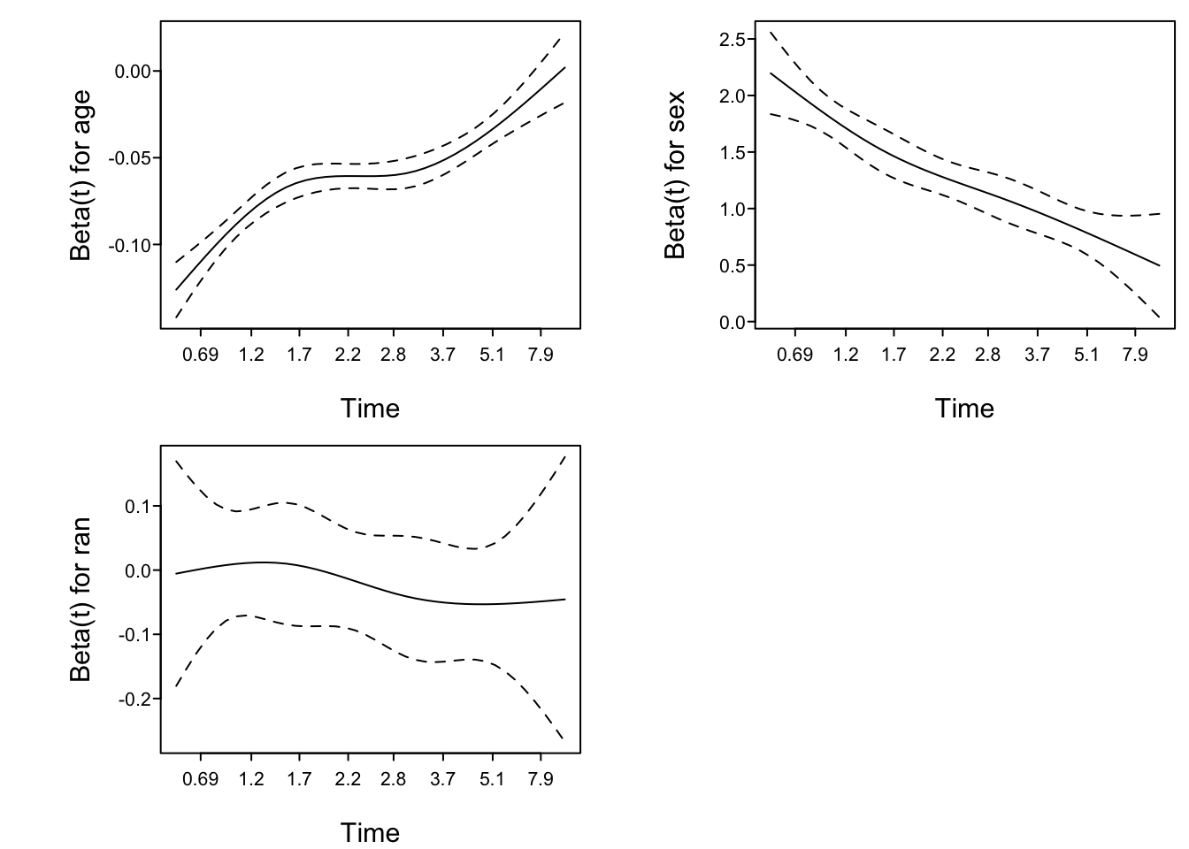
Code
ord_ints <- coef(g11)[1 : num.intercepts(g11)]
cox_ints <- f11$surv
cox_ints <- log(-log(cox_ints[-c(1, length(cox_ints))]))
ggplot(mapping=aes(x=ord_ints, y=cox_ints)) + geom_line() +
  xlab('orm Intercepts') + ylab('Cox Intercepts')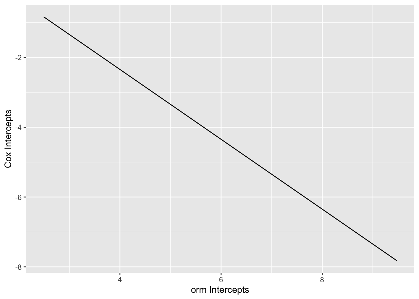
Code
f <- lm(cox_ints ~ ord_ints)
coef(f)
(Intercept) ord_ints
1.6530871 -0.9999025 Code
mean(abs(resid(f)))[1] 8.616624e-0525.8.2 Data from Log-logistic AFT Model With Non-PH
Examine parallelism of transformed Kaplan-Meier estimates stratified by intervals of the true linear predictor.
Code
# Compute the number of events per lp group
table(t2 <= cens, g)
g
-0.37 0.2 0.65 1.24
FALSE 10 44 73 176
TRUE 490 456 427 324Code
f <- npsurv(S2 ~ g)
ggplot(f, trans='loglog', logt=TRUE, conf='none') + labs(title='log-log Link')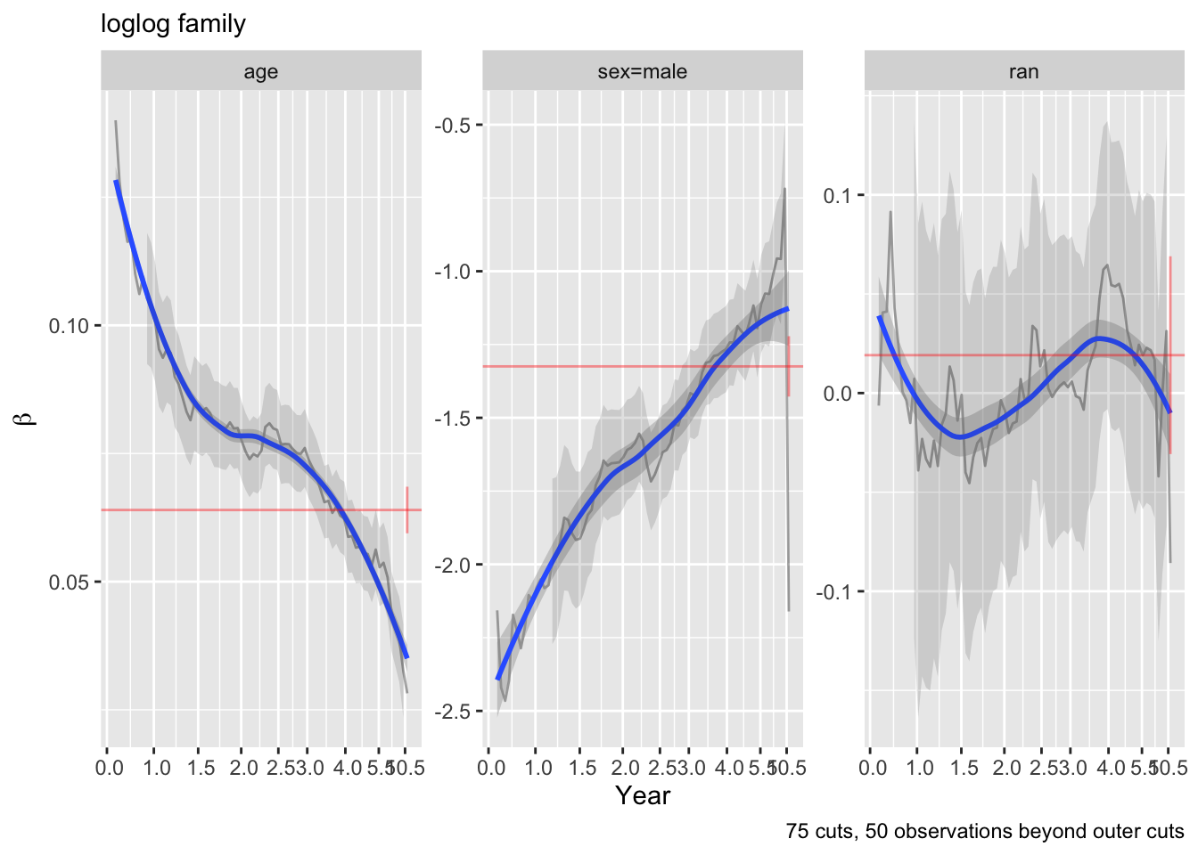
Code
ggplot(f, trans='logit', logt=TRUE, conf='none') + labs(title='logit Link')
Code
ggplot(f, trans='probit', logt=TRUE, conf='none') + labs(title='probit link')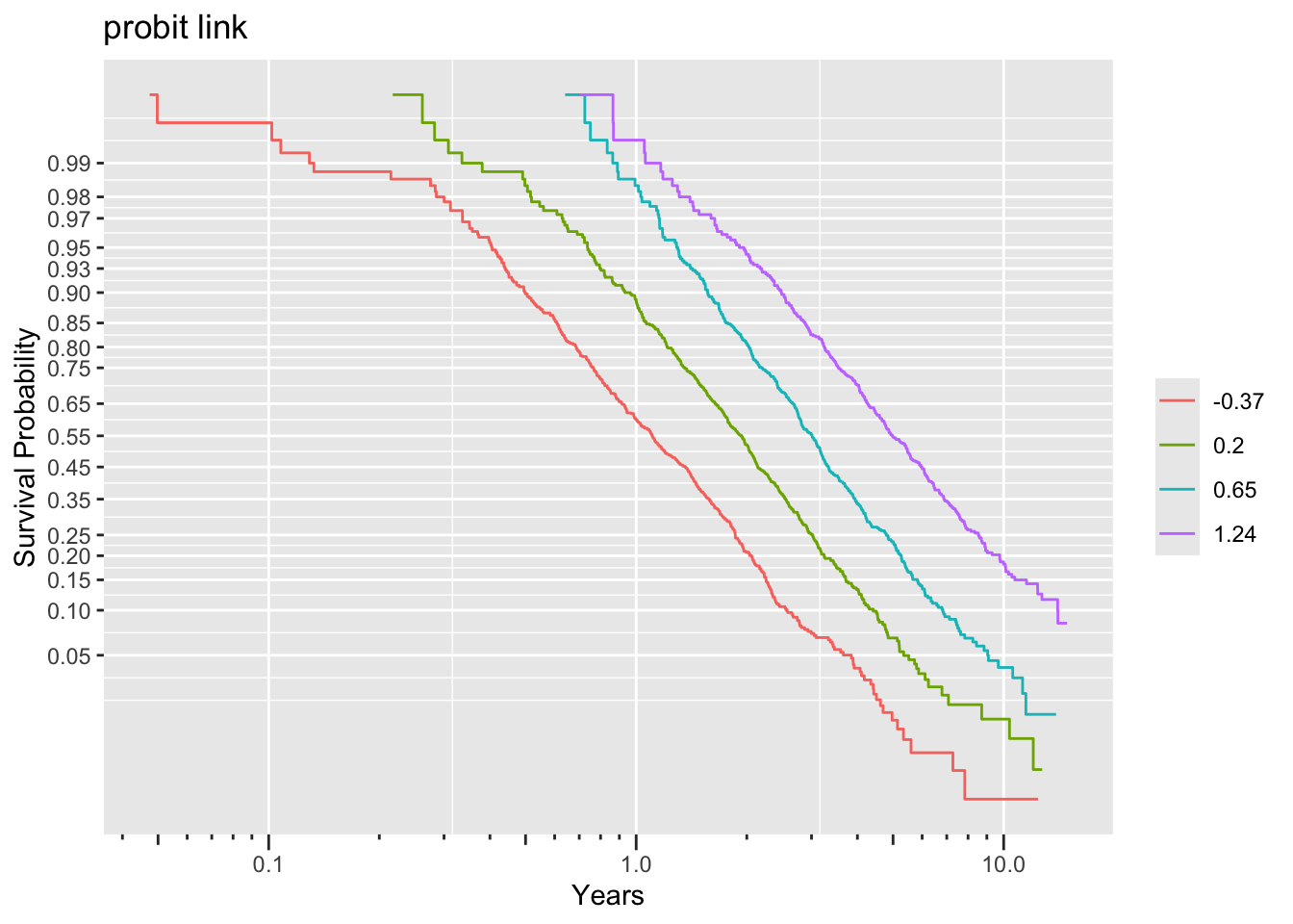
The Cox model (log-log link) clearly fits less well than the two AFTs.
Compare regression coefficients and standard errors.
Code
fits <- list(Cox=f21, loglog=g21, logit=g22)
maketabs(fits)
Cox Proportional Hazards Model
cph(formula = S2 ~ age + sex + ran, x = TRUE, y = TRUE, surv = TRUE)
| Model Tests | Discrimination Indexes |
|
|---|---|---|
| Obs 2000 | LR χ2 1198.73 | R2 0.451 |
| Events 1697 | d.f. 3 | R23,2000 0.450 |
| Center -2.5779 | Pr(>χ2) 0.0000 | R23,1697 0.506 |
| Score χ2 1196.09 | Dxy 0.543 | |
| Pr(>χ2) 0.0000 |
| β | S.E. | Wald Z | Pr(>|Z|) | |
|---|---|---|---|---|
| age | -0.0639 | 0.0023 | -27.57 | <0.0001 |
| sex=male | 1.3238 | 0.0525 | 25.20 | <0.0001 |
| ran | -0.0190 | 0.0255 | -0.75 | 0.4554 |
-log-log Ordinal Regression Model
orm(formula = Y2 ~ age + sex + ran, family = "loglog", x = TRUE,
    y = TRUE, mscore = TRUE)
| Model Likelihood Ratio Test |
Discrimination Indexes |
Rank Discrim. Indexes |
|
|---|---|---|---|
| Obs 2000 | LR χ2 1200.12 | R2 0.451 | Dxy 0.543 |
| ESS 1740.2 | d.f. 3 | R23,2000 0.450 | |
| Censored R=303 | Pr(>χ2) <0.0001 | R23,1740.2 0.497 | |
| Distinct Y 1698 | Score χ2 1197.53 | |Pr(Y ≥ median)-½| 0.236 | |
| Y0.5 2.166504 | Pr(>χ2) <0.0001 | ||
| max |∂log L/∂β| 4×10⁻¹⁰ |
| β | S.E. | Wald Z | Pr(>|Z|) | |
|---|---|---|---|---|
| age | 0.0640 | 0.0023 | 27.59 | <0.0001 |
| sex=male | -1.3246 | 0.0525 | -25.22 | <0.0001 |
| ran | 0.0191 | 0.0255 | 0.75 | 0.4529 |
Logistic (Proportional Odds) Ordinal Regression Model
orm(formula = Y2 ~ age + sex + ran, family = "logistic", x = TRUE,
    y = TRUE, mscore = TRUE)
| Model Likelihood Ratio Test |
Discrimination Indexes |
Rank Discrim. Indexes |
|
|---|---|---|---|
| Obs 2000 | LR χ2 1416.98 | R2 0.508 | Dxy 0.543 |
| ESS 1739.3 | d.f. 3 | R23,2000 0.507 | |
| Censored R=303 | Pr(>χ2) <0.0001 | R23,1739.3 0.556 | |
| Distinct Y 1698 | Score χ2 1471.54 | |Pr(Y ≥ median)-½| 0.276 | |
| Y0.5 2.166504 | Pr(>χ2) <0.0001 | ||
| max |∂log L/∂β| 1×10⁻⁹ |
| β | S.E. | Wald Z | Pr(>|Z|) | |
|---|---|---|---|---|
| age | 0.1163 | 0.0040 | 28.78 | <0.0001 |
| sex=male | -2.3511 | 0.0918 | -25.62 | <0.0001 |
| ran | -0.0004 | 0.0409 | -0.01 | 0.9918 |
Code
cbetas(fits)betas:
Cox loglog logit
age -0.06393658 0.06397676 0.1163000629
sex=male 1.32378760 -1.32461605 -2.3511015761
ran -0.01900550 0.01911016 -0.0004206686
Correlations of linear predictors:
Cox loglog logit
Cox 1.00000 -1.00000 -0.99977
loglog -1.00000 1.00000 0.99976
logit -0.99977 0.99976 1.00000
Cox: standard errors from information matrix and robust sandwich estimator
age sex=male ran
Info 0.0023 0.0525 0.0255
Robust 0.0028 0.0645 0.0298
loglog: standard errors from information matrix and robust sandwich estimator
age sex=male ran
Info 0.0023 0.0525 0.0255
Robust 0.0028 0.0646 0.0298
logit: standard errors from information matrix and robust sandwich estimator
age sex=male ran
Info 0.0040 0.0918 0.0409
Robust 0.0041 0.0906 0.0414Check parallelism assumptions.
Code
czph(f21)cox.zph tests for proportional hazards
chisq df p
age 79.57 1 <2e-16
sex 41.78 1 1e-10
ran 1.14 1 0.29
GLOBAL 146.29 3 <2e-16
Code
ordParallel(g21)
ordParallel(g22)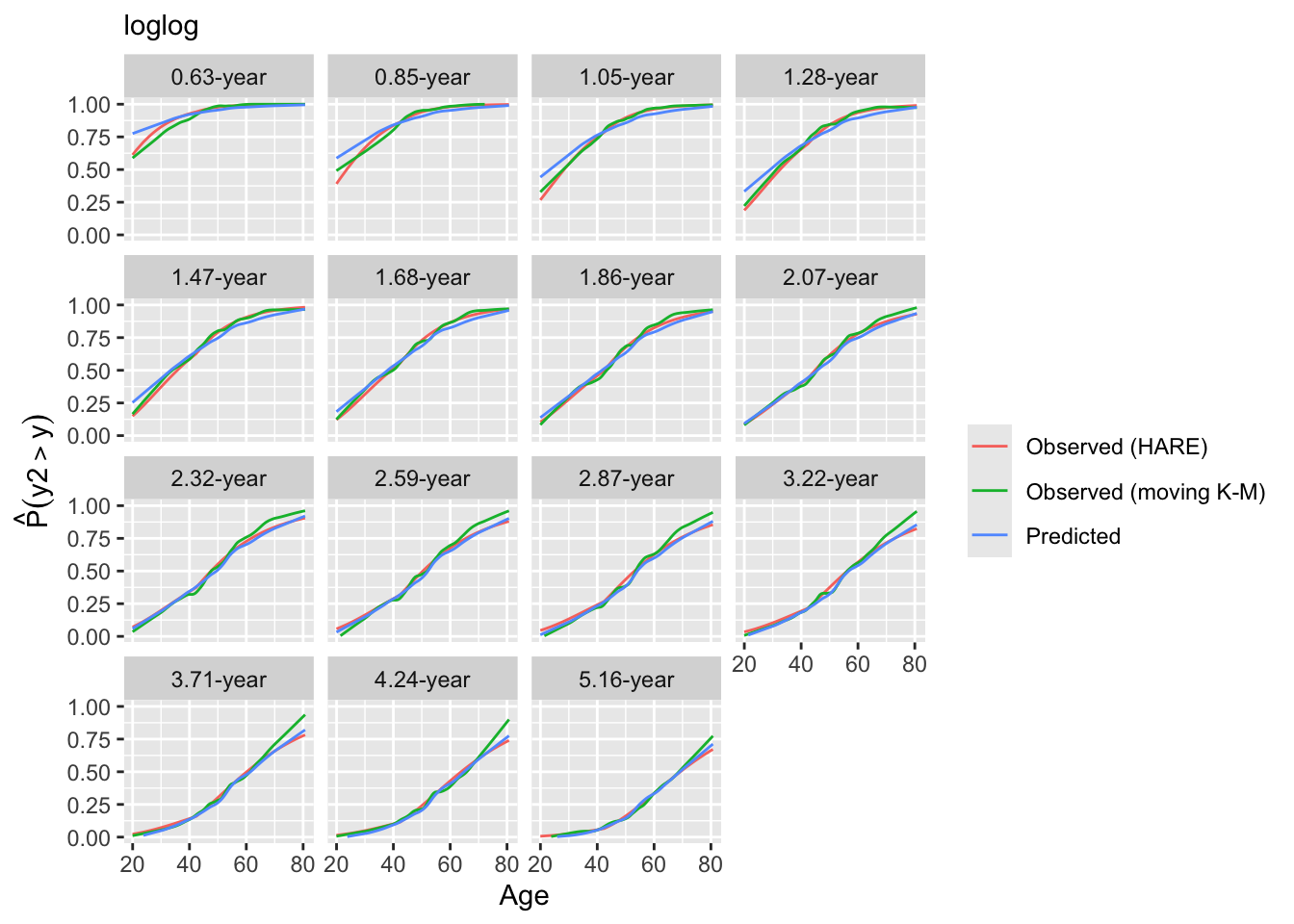
Cox and the ordinal regression version of Cox with log-log link fail to properly model the covariate effects, with the Cox cox.zph tests of PH yielding an overall \(\chi^{2}_{3} = 146\).
Now do this for just the linear predictor \(X\hat{\beta}\).
Code
ordParallel(g21, lp=TRUE)
ordParallel(g22, lp=TRUE)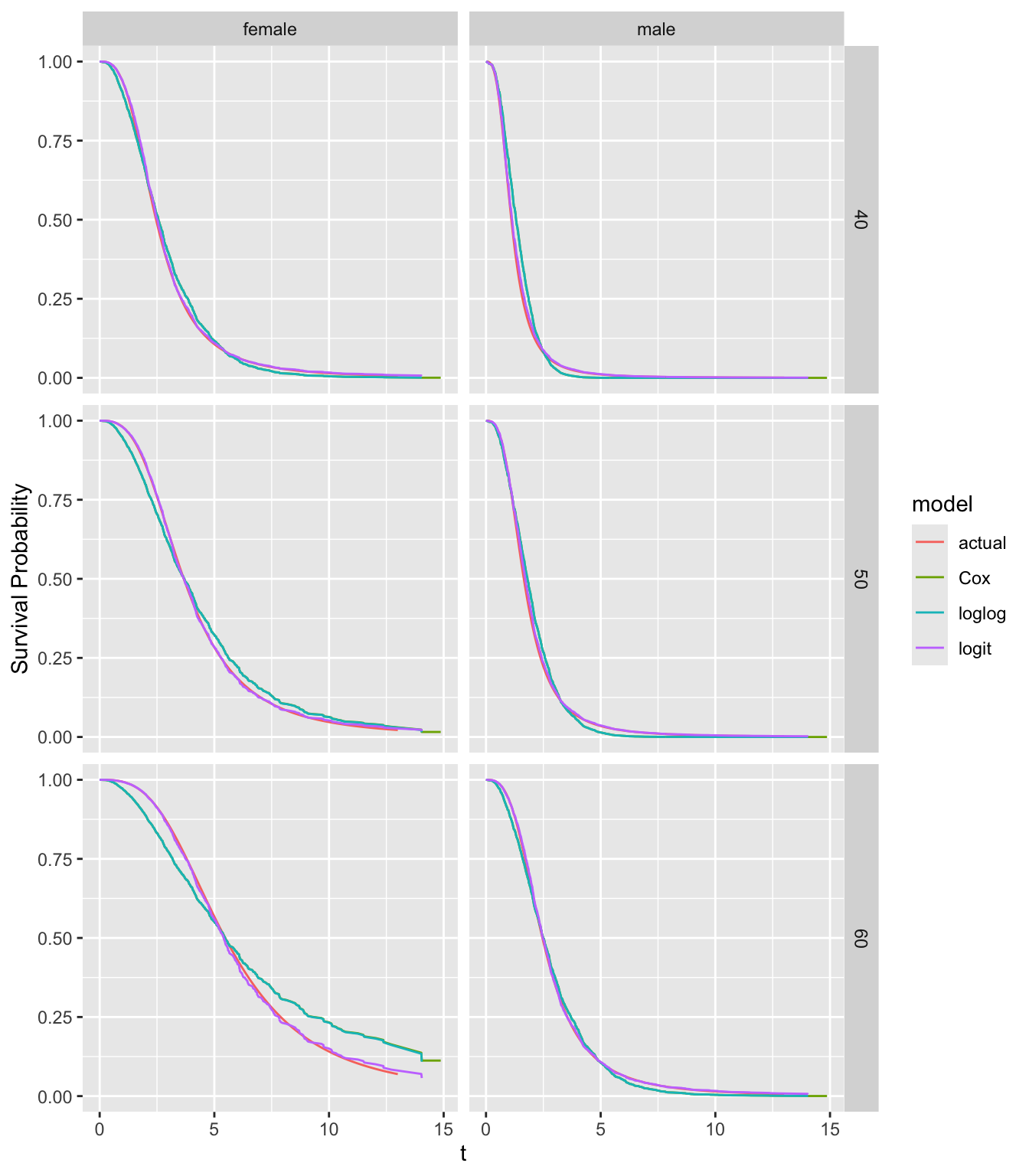
Look at internal calibrations.
Code
intCalibration(g21, m=200, dec=2) + labs(subtitle=g21$family)
Calibration-in-the-large:

    y Mean Predicted P(Y > y) Observed P(Y > y)
 0.85                  0.8942            0.8995
 1.28                  0.7870            0.7990
 1.68                  0.6808            0.6975
 2.07                  0.5810            0.5999
 2.59                  0.4761            0.4976
 3.22                  0.3712            0.3911
 4.24                  0.2618            0.2722
Code
intCalibration(g22, m=200, dec=2) + labs(subtitle=g22$family)
Calibration-in-the-large:

    y Mean Predicted P(Y > y) Observed P(Y > y)
 0.85                  0.8973            0.8995
 1.28                  0.7950            0.7990
 1.68                  0.6947            0.6975
 2.07                  0.5985            0.5999
 2.59                  0.4941            0.4976
 3.22                  0.3868            0.3911
 4.24                  0.2701            0.2722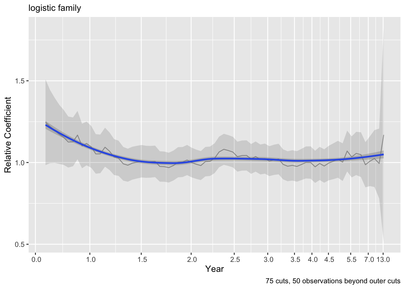
The logit link is decidedly better by the plots of predicted vs. observed probabilities.
We can also check calibration with respect to age.
Code
intCalibration(g21, m=100, x=age, hare=FALSE, dec=2) +
  labs(subtitle=g21$family)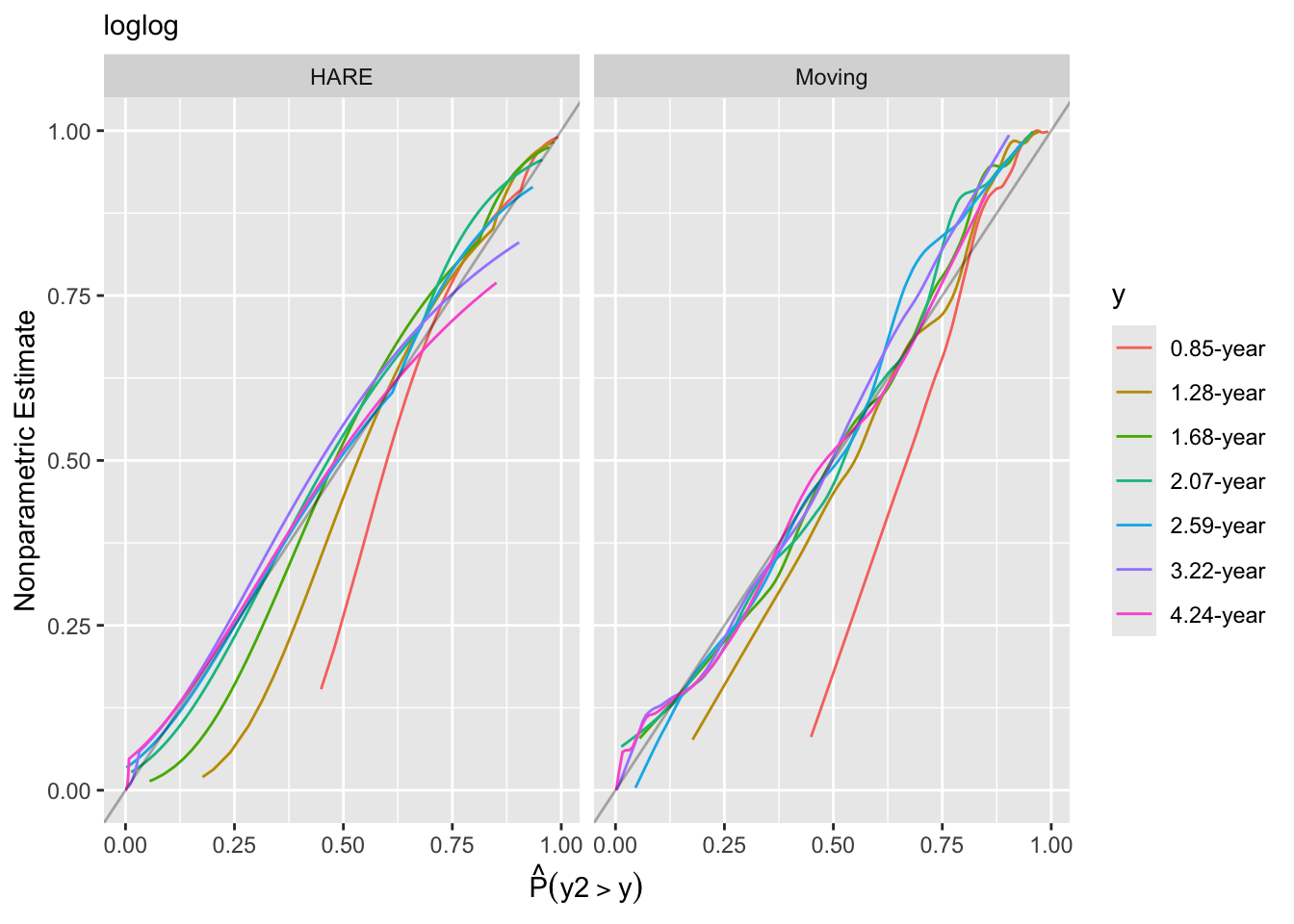
Code
intCalibration(g22, m=100, x=age, hare=FALSE, dec=2) +
  labs(subtitle=g22$family)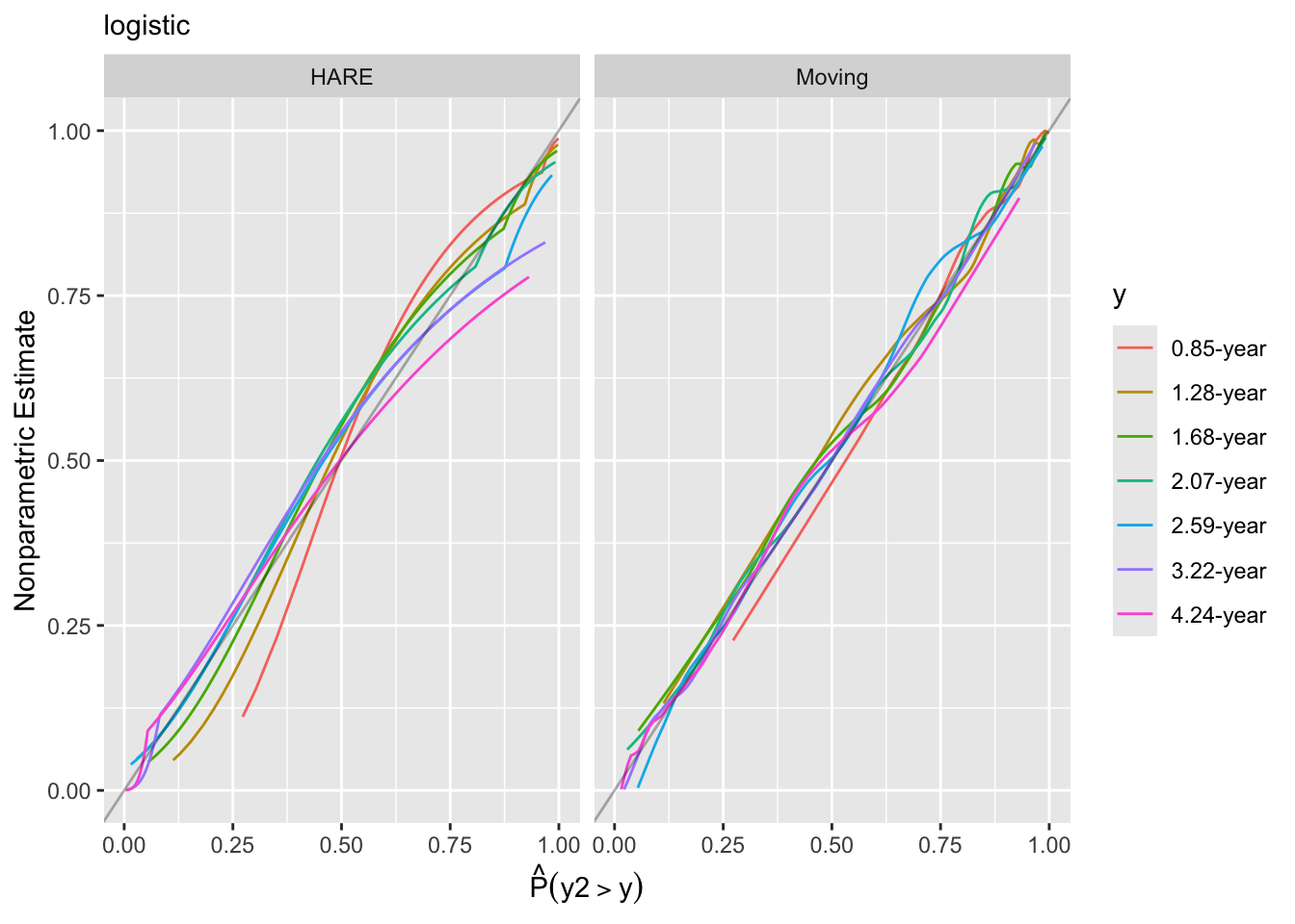
Check the deviance and other measures for several links.
Code
Olinks(g21) link null.deviance deviance AIC LR R2
1 loglog 26321.79 25121.67 28521.67 1200.119 0.497
2 logistic 26321.79 24904.80 28304.80 1416.983 0.556
3 probit 26321.79 24908.80 28308.80 1412.988 0.555
4 cloglog 26321.79 25068.89 28468.89 1252.900 0.513Fortunately, the logit link had smaller deviance (and AIC).
Get predicted survival curves and compare them to the actual survival functions used to simulate the data, as before. The true survival function is as follows, with \(X\beta =\) 0.5 plus the original linear predictor lp and \(r\) is a random variable from a standard logistic distribution.
\[S(t) = P(T > t) = P(\exp(X\beta + \frac{r}{3}) > t) = P(X\beta + \frac{r}{3} > \log(t)) = 1 - \text{expit}(3(\log(t) - X\beta))\]
Code
S_actual <- function(age, sex, ran=0) {
  times <- seq(.02, 13, length=200)
  lp <- 0.5 + 0.04 * (age - 50) + 0.8 * (sex == 'female')
  s <- 1 - plogis(3*(log(times) - lp))
  data.frame(time=times, surv=s)
}
fits <- list(actual=S_actual, Cox=f21, loglog=g21, logit=g22)
compsurv(fits)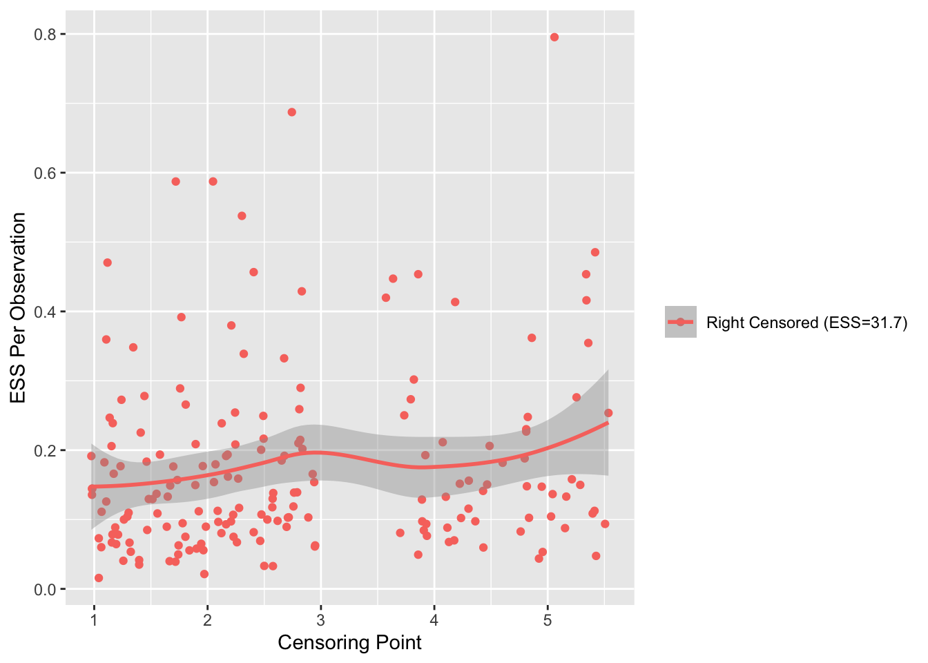
The Cox and ordinal semiparametric log-log link estimates are indistinguishable. The logit link estimates and the true survival curves are almost indistinguishable. The Cox and log-log estimates, which both falsely assume PH, do not agree with the true curves, especially for 60 year-old females.
Note that log hazard ratios are moving towards zero as \(t\uparrow\). When data come from an AFT distribution that has a non-PH form, the true hazard ratios converge to 1.0, i.e, covariate effects wear off on the hazard ratio scale.
25.9 Accelerated Failure Time Example
Consider the SUPPORT dataset analysed with a parametric log-logistic AFT model in Chapter 19. In ordinal models we do not have the same kind of residual plots for checking distributional assumptions, because there is no assumption about the distribution of absolute failure time \(T\) given a set of covariate values \(X\). We do have a parallelism assumption. Along the lines of this in Chapter 15 let’s fit a rough model and divide predictions into intervals of 80 patients. Then let’s see if logit of Kaplan-Meier curves are parallel.
Fit the smaller model near the end of Chapter 19.
Code
getHdata(support)          # Get data frame from web site
acute     <- support$dzclass %in% c('ARF/MOSF','Coma')
d         <- support[acute, ]
d$dzgroup <- d$dzgroup[drop=TRUE]    # Remove unused levels
d <- upData(d, print=FALSE,
       t = d.time/365.25,
       labels = c(t = 'Survival Time'),
  units = c(t = 'year'))
d <- upData(d,
        Y = Ocens(t, ifelse(death == 1, t, Inf)))
Input object size: 167280 bytes; 36 variables 537 observations
Added variable Y
New object size: 177416 bytes; 37 variables 537 observationsCode
maxuc <- with(d, max(t[death == 1]))
round(maxuc, 3)
[1] 4.4Code
minc  <- round(with(d, min(t[t > maxuc])), 2)
minc
[1] 4.43Code
with(d, sum(t[death == 0] > 4.399726))[1] 33Code
c(censored=sum(d$death), uncensored=nrow(d) - sum(d$death)) censored uncensored
356 181 Do simple single imputation.
Code
d <- upData(d, print=FALSE,
  wblc = impute(wblc, 9),
  pafi = impute(pafi, 333.3),
  ph   = impute(ph,   7.4),
  race2  = ifelse(is.na(race), 'white',
                  ifelse(race != 'white', 'other', 'white')) )
dd <- datadist(d); options(datadist='dd')
Fit the semiparametric generalization of the log-normal AFT model.
Code
f <- orm(Y ~ dzgroup + rcs(meanbp,5) + rcs(crea,4) + rcs(age,5) +
         rcs(hrt,3) + scoma + rcs(pafi,4) + pol(adlsc,2) +
         rcs(resp,3), family='probit', data=d, x=TRUE, y=TRUE, lpe=TRUE, trace=1)
NR iteration:1 -2LL:3944.7503 Max |gradient|:3.728847e-11 Max |change in parameters|:1.220769e-15
NR iteration:1 -2LL:3944.7503 Max |gradient|:7318.883 Max |change in parameters|:13.00543
NR iteration:2 -2LL:3666.4279 Max |gradient|:1889.741 Max |change in parameters|:0.5601498
NR iteration:3 -2LL:3662.7147 Max |gradient|:24.24805 Max |change in parameters|:0.08309238
NR iteration:4 -2LL:3662.6834 Max |gradient|:0.2031274 Max |change in parameters|:0.001485343
NR iteration:5 -2LL:3662.6834 Max |gradient|:9.059911e-05 Max |change in parameters|:6.691449e-07Code
fProbit Ordinal Regression Model
orm(formula = Y ~ dzgroup + rcs(meanbp, 5) + rcs(crea, 4) + rcs(age,
    5) + rcs(hrt, 3) + scoma + rcs(pafi, 4) + pol(adlsc, 2) +
    rcs(resp, 3), data = d, family = "probit", x = TRUE, y = TRUE,
    lpe = TRUE, trace = 1)
| Model Likelihood Ratio Test |
Discrimination Indexes |
Rank Discrim. Indexes |
|
|---|---|---|---|
| Obs 537 | LR χ2 282.07 | R2 0.409 | Dxy 0.481 |
| ESS 380.5 | d.f. 23 | R223,537 0.383 | |
| Censored R=181 | Pr(>χ2) <0.0001 | R223,380.5 0.494 | |
| Distinct Y 176 | Score χ2 266.32 | |Pr(Y ≥ median)-½| 0.264 | |
| Y0.5 0.0684463 | Pr(>χ2) <0.0001 | ||
| max |∂log L/∂β| 3×10⁻¹⁰ |
| β | S.E. | Wald Z | Pr(>|Z|) | |
|---|---|---|---|---|
| dzgroup=Coma | -0.8986 | 0.1835 | -4.90 | <0.0001 |
| dzgroup=MOSF w/Malig | -0.8439 | 0.1303 | -6.48 | <0.0001 |
| meanbp | 0.0572 | 0.0104 | 5.48 | <0.0001 |
| meanbp' | -0.3063 | 0.1068 | -2.87 | 0.0041 |
| meanbp'' | 0.8955 | 0.3979 | 2.25 | 0.0244 |
| meanbp''' | -0.6439 | 0.3545 | -1.82 | 0.0693 |
| crea | -0.1811 | 0.2953 | -0.61 | 0.5397 |
| crea' | -7.3578 | 8.3936 | -0.88 | 0.3807 |
| crea'' | 13.6502 | 13.7063 | 1.00 | 0.3193 |
| age | -0.0116 | 0.0140 | -0.83 | 0.4064 |
| age' | -0.0070 | 0.0488 | -0.14 | 0.8866 |
| age'' | 0.0269 | 0.2521 | 0.11 | 0.9150 |
| age''' | 0.0233 | 0.6163 | 0.04 | 0.9699 |
| hrt | -0.0048 | 0.0031 | -1.57 | 0.1168 |
| hrt' | 0.0010 | 0.0028 | 0.34 | 0.7350 |
| scoma | -0.0072 | 0.0020 | -3.66 | 0.0003 |
| pafi | 0.0085 | 0.0025 | 3.44 | 0.0006 |
| pafi' | -0.0265 | 0.0107 | -2.49 | 0.0129 |
| pafi'' | 0.0490 | 0.0215 | 2.28 | 0.0225 |
| adlsc | -0.1783 | 0.0683 | -2.61 | 0.0090 |
| adlsc2 | 0.0202 | 0.0110 | 1.84 | 0.0653 |
| resp | 0.0242 | 0.0104 | 2.32 | 0.0203 |
| resp' | -0.0391 | 0.0131 | -2.98 | 0.0029 |
Code
a <- anova(f, test='LR')
plot(a)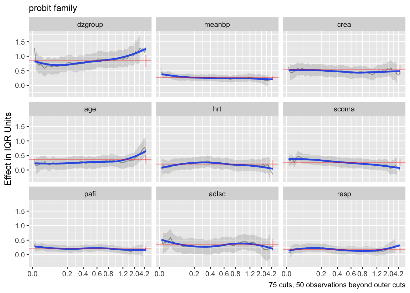
The first output from trace=1 shows the maximum likelihood iterative process when there are no predictors in the model, only intercepts. Notice that the iterations had already converged at the starting values, which were normal inverses of the Kaplan-Meier estimates. So the maximum likelihood estimates in an ordinal semiparametric model are exactly the link function of the Kaplan-Meier estimates when there are no covariates.
When there are right-censored observations above the highest uncensored time, Ocens2ord creates a new level for them and considers them to be uncensored at the lowest of such times. This is because these are high-information points, and treating them this way still makes orm result in K-M estimates with no covariates. But the numbers of censored observations reported in the output are the actual numbers before this modification.
There are 356 deaths. The effective sample size is estimated to be 380.5, i.e., the number of complete observations that would provide the same statistical information as the 537 observations with 181 right-censored. We can look at the information in right-censored observations in detail by using the rms ordESS function to plot the effective sample size vs. censoring time. We expect late-censored observations to provide more information than early-censored ones.
Code
ordESS(f)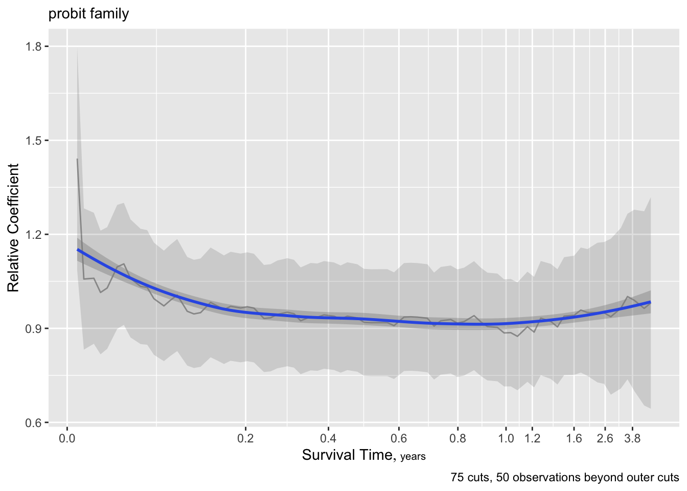
We see a slight increase in the ESS for longer follow-up times. Altogether the 181 right-censored observations have the information of 24.5 uncensored times.
Plot the model intercepts, which represent the survival curve for persons with all covariates equal to zero, on the probit scale with time log-transformed.
Code
plotIntercepts(f, logt=TRUE)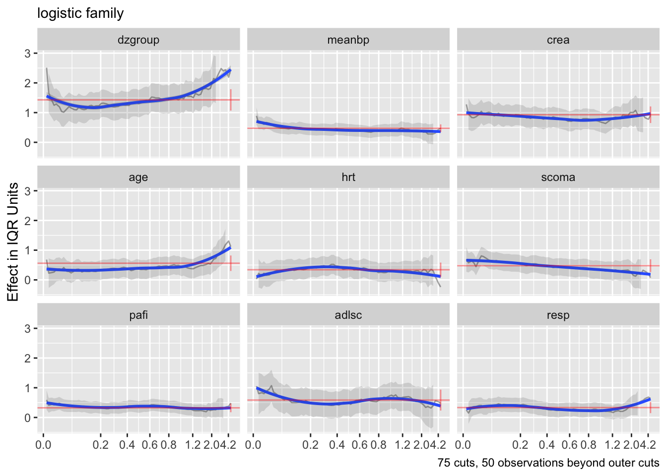
This is not quite straight, indicating that a log-normal AFT model would not be perfect, e.g., the \(\log(t)\) transformation part of the model may be wrong.
Unlike the parametric model we do not need such curves to be linear, only parallel across covariate values.
There are two other ways to check model assumptions, one of which is to estimate \(\beta(t)\) and check for flatness (irrelevance of \(t\)). Do this for the probit fit.
Code
ordParallel(f)
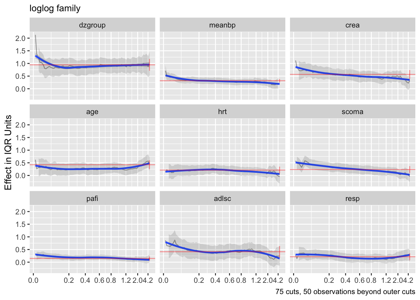
The curves are fairly flat. But it is difficult to interpret trends in individual \(\beta\) that make up one predictor’s effect. Use an option to compute the partial linear predictor for each of the model’s predictors. Each weighted sum term gives rise to an effect that now has \(\beta=1\). The terms are scaled so that they are in units of inter-quartile range of the part of linear predictor involving a predictor. In this way a weak variable will have a smaller effect. See how the overall multiplier varies as a function of time. This does not allow for shape changes over time but does allow change in overall importance (steepness).
Code
ordParallel(f, terms=TRUE)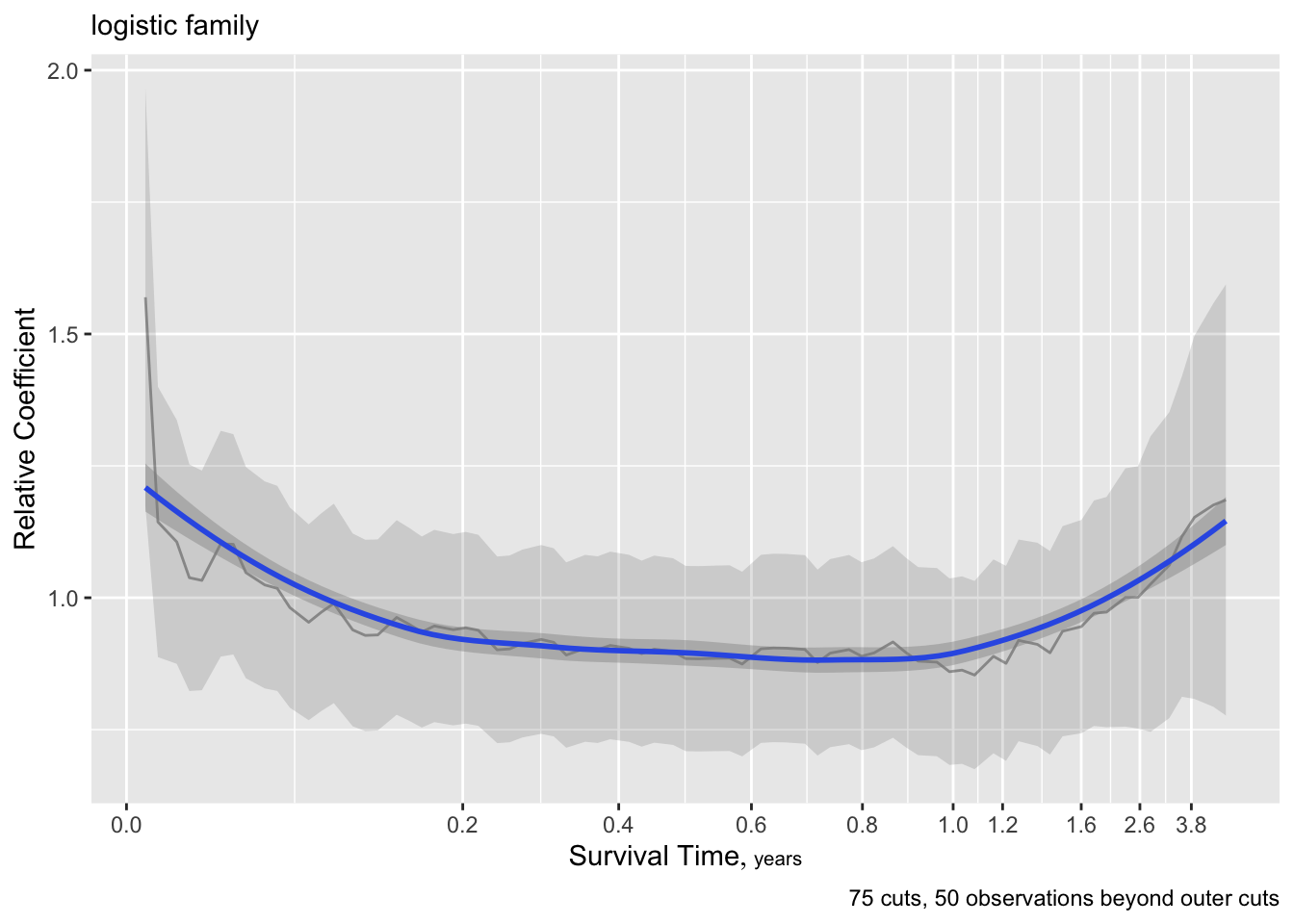
Also do this for the overall linear predictor.
Code
ordParallel(f, lp=TRUE)
There seems to e an increasing effect of age over time, and a decreasing effect of coma score.
Let’s see how some other link functions fare.
Code
g <- update(f, family='logistic', trace=0)
ordParallel(g, terms=TRUE)
Code
h <- update(g, family='loglog')
ordParallel(h, terms=TRUE)
Code
ordParallel(g, lp=TRUE)
ordParallel(h, lp=TRUE)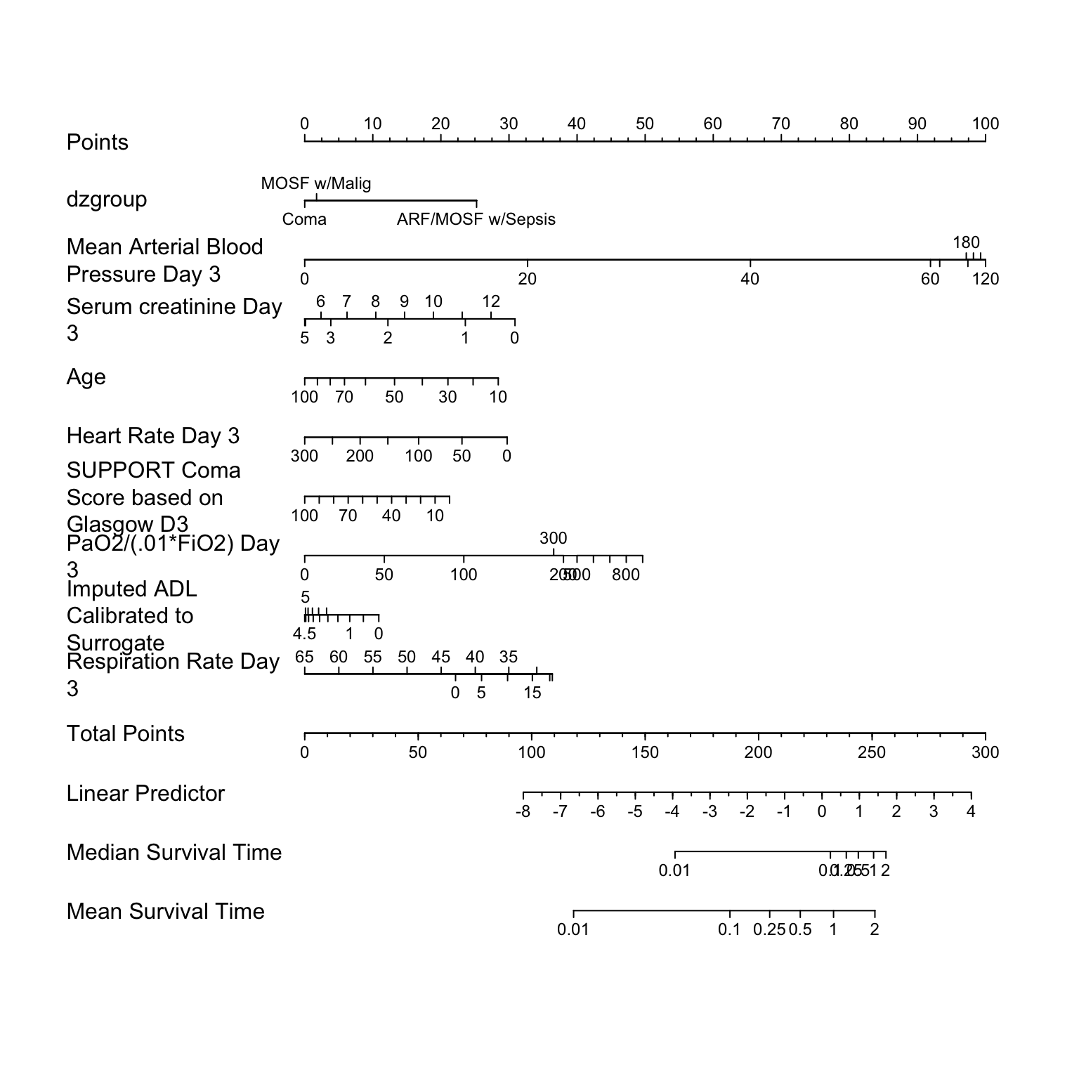
Do formal tests of goodness-of-link (parallelism on the assumed link scale) by having ordParallel create 30 copies of the dataset with different cutoffs of survival time, and when censoring allows, determine whether observed survival time exceeds the cutoff. The global multiplicity-adjusted test for parallelism is in the TOTAL INTERACTION line near the bottom of each ANOVA.
Code
testpar <- function(form, link) {
  f  <- orm(form, data=d, family=link, x=TRUE, y=TRUE)
  do <- ordParallel(f, onlydata=TRUE, maxcuts=30)
  g  <- orm(Yge_cut ~ (dzgroup + meanbp + crea + age + hrt +
                         scoma + pafi + adlsc + resp) * rcs(Ycut, 3),
            data=do, family=link, x=TRUE, y=TRUE)
  h  <- robcov(g, do$obs)
  anova(h)
}
form <- Y ~ dzgroup + rcs(meanbp, 5) + rcs(crea, 4) + rcs(age, 5) + rcs(hrt, 3) +
  scoma + rcs(pafi, 4) + pol(adlsc, 2) + rcs(resp, 3)
fams <- .q(probit, logistic, loglog)
w <- lapply(fams, function(x) testpar(form, x))
names(w) <- fams
maketabs(w)Wald Statistics for Yge_cut |
|||
| χ2 | d.f. | P | |
|---|---|---|---|
| dzgroup (Factor+Higher Order Factors) | 173.66 | 3 | <0.0001 |
| All Interactions | 25.11 | 2 | <0.0001 |
| meanbp (Factor+Higher Order Factors) | 145.40 | 3 | <0.0001 |
| All Interactions | 3.38 | 2 | 0.1843 |
| crea (Factor+Higher Order Factors) | 98.05 | 3 | <0.0001 |
| All Interactions | 0.00 | 2 | 0.9998 |
| age (Factor+Higher Order Factors) | 60.55 | 3 | <0.0001 |
| All Interactions | 23.38 | 2 | <0.0001 |
| hrt (Factor+Higher Order Factors) | 19.10 | 3 | 0.0003 |
| All Interactions | 5.95 | 2 | 0.0510 |
| scoma (Factor+Higher Order Factors) | 76.04 | 3 | <0.0001 |
| All Interactions | 17.86 | 2 | 0.0001 |
| pafi (Factor+Higher Order Factors) | 55.46 | 3 | <0.0001 |
| All Interactions | 2.54 | 2 | 0.2810 |
| adlsc (Factor+Higher Order Factors) | 25.77 | 3 | <0.0001 |
| All Interactions | 4.69 | 2 | 0.0960 |
| resp (Factor+Higher Order Factors) | 61.15 | 3 | <0.0001 |
| All Interactions | 10.23 | 2 | 0.0060 |
| Ycut (Factor+Higher Order Factors) | 1848.64 | 20 | <0.0001 |
| All Interactions | 100.56 | 18 | <0.0001 |
| Nonlinear (Factor+Higher Order Factors) | 350.46 | 10 | <0.0001 |
| dzgroup × Ycut (Factor+Higher Order Factors) | 25.11 | 2 | <0.0001 |
| Nonlinear | 8.55 | 1 | 0.0035 |
| Nonlinear Interaction : f(A,B) vs. AB | 8.55 | 1 | 0.0035 |
| meanbp × Ycut (Factor+Higher Order Factors) | 3.38 | 2 | 0.1843 |
| Nonlinear | 0.10 | 1 | 0.7544 |
| Nonlinear Interaction : f(A,B) vs. AB | 0.10 | 1 | 0.7544 |
| crea × Ycut (Factor+Higher Order Factors) | 0.00 | 2 | 0.9998 |
| Nonlinear | 0.00 | 1 | 0.9849 |
| Nonlinear Interaction : f(A,B) vs. AB | 0.00 | 1 | 0.9849 |
| age × Ycut (Factor+Higher Order Factors) | 23.38 | 2 | <0.0001 |
| Nonlinear | 0.06 | 1 | 0.8009 |
| Nonlinear Interaction : f(A,B) vs. AB | 0.06 | 1 | 0.8009 |
| hrt × Ycut (Factor+Higher Order Factors) | 5.95 | 2 | 0.0510 |
| Nonlinear | 1.52 | 1 | 0.2180 |
| Nonlinear Interaction : f(A,B) vs. AB | 1.52 | 1 | 0.2180 |
| scoma × Ycut (Factor+Higher Order Factors) | 17.86 | 2 | 0.0001 |
| Nonlinear | 3.94 | 1 | 0.0471 |
| Nonlinear Interaction : f(A,B) vs. AB | 3.94 | 1 | 0.0471 |
| pafi × Ycut (Factor+Higher Order Factors) | 2.54 | 2 | 0.2810 |
| Nonlinear | 0.01 | 1 | 0.9335 |
| Nonlinear Interaction : f(A,B) vs. AB | 0.01 | 1 | 0.9335 |
| adlsc × Ycut (Factor+Higher Order Factors) | 4.69 | 2 | 0.0960 |
| Nonlinear | 3.32 | 1 | 0.0682 |
| Nonlinear Interaction : f(A,B) vs. AB | 3.32 | 1 | 0.0682 |
| resp × Ycut (Factor+Higher Order Factors) | 10.23 | 2 | 0.0060 |
| Nonlinear | 9.15 | 1 | 0.0025 |
| Nonlinear Interaction : f(A,B) vs. AB | 9.15 | 1 | 0.0025 |
| TOTAL NONLINEAR | 350.46 | 10 | <0.0001 |
| TOTAL INTERACTION | 100.56 | 18 | <0.0001 |
| TOTAL NONLINEAR + INTERACTION | 464.89 | 19 | <0.0001 |
| TOTAL | 2299.21 | 29 | <0.0001 |
Wald Statistics for Yge_cut |
|||
| χ2 | d.f. | P | |
|---|---|---|---|
| dzgroup (Factor+Higher Order Factors) | 48.06 | 3 | <0.0001 |
| All Interactions | 8.06 | 2 | 0.0178 |
| meanbp (Factor+Higher Order Factors) | 46.57 | 3 | <0.0001 |
| All Interactions | 0.74 | 2 | 0.6922 |
| crea (Factor+Higher Order Factors) | 31.91 | 3 | <0.0001 |
| All Interactions | 0.10 | 2 | 0.9521 |
| age (Factor+Higher Order Factors) | 20.65 | 3 | 0.0001 |
| All Interactions | 9.78 | 2 | 0.0075 |
| hrt (Factor+Higher Order Factors) | 6.81 | 3 | 0.0780 |
| All Interactions | 1.52 | 2 | 0.4680 |
| scoma (Factor+Higher Order Factors) | 25.06 | 3 | <0.0001 |
| All Interactions | 2.79 | 2 | 0.2478 |
| pafi (Factor+Higher Order Factors) | 19.48 | 3 | 0.0002 |
| All Interactions | 0.32 | 2 | 0.8534 |
| adlsc (Factor+Higher Order Factors) | 8.62 | 3 | 0.0348 |
| All Interactions | 0.95 | 2 | 0.6220 |
| resp (Factor+Higher Order Factors) | 18.70 | 3 | 0.0003 |
| All Interactions | 3.32 | 2 | 0.1901 |
| Ycut (Factor+Higher Order Factors) | 471.19 | 20 | <0.0001 |
| All Interactions | 31.00 | 18 | 0.0288 |
| Nonlinear (Factor+Higher Order Factors) | 109.56 | 10 | <0.0001 |
| dzgroup × Ycut (Factor+Higher Order Factors) | 8.06 | 2 | 0.0178 |
| Nonlinear | 2.13 | 1 | 0.1449 |
| Nonlinear Interaction : f(A,B) vs. AB | 2.13 | 1 | 0.1449 |
| meanbp × Ycut (Factor+Higher Order Factors) | 0.74 | 2 | 0.6922 |
| Nonlinear | 0.08 | 1 | 0.7742 |
| Nonlinear Interaction : f(A,B) vs. AB | 0.08 | 1 | 0.7742 |
| crea × Ycut (Factor+Higher Order Factors) | 0.10 | 2 | 0.9521 |
| Nonlinear | 0.00 | 1 | 0.9470 |
| Nonlinear Interaction : f(A,B) vs. AB | 0.00 | 1 | 0.9470 |
| age × Ycut (Factor+Higher Order Factors) | 9.78 | 2 | 0.0075 |
| Nonlinear | 0.01 | 1 | 0.9176 |
| Nonlinear Interaction : f(A,B) vs. AB | 0.01 | 1 | 0.9176 |
| hrt × Ycut (Factor+Higher Order Factors) | 1.52 | 2 | 0.4680 |
| Nonlinear | 0.68 | 1 | 0.4109 |
| Nonlinear Interaction : f(A,B) vs. AB | 0.68 | 1 | 0.4109 |
| scoma × Ycut (Factor+Higher Order Factors) | 2.79 | 2 | 0.2478 |
| Nonlinear | 0.76 | 1 | 0.3831 |
| Nonlinear Interaction : f(A,B) vs. AB | 0.76 | 1 | 0.3831 |
| pafi × Ycut (Factor+Higher Order Factors) | 0.32 | 2 | 0.8534 |
| Nonlinear | 0.00 | 1 | 0.9846 |
| Nonlinear Interaction : f(A,B) vs. AB | 0.00 | 1 | 0.9846 |
| adlsc × Ycut (Factor+Higher Order Factors) | 0.95 | 2 | 0.6220 |
| Nonlinear | 0.67 | 1 | 0.4124 |
| Nonlinear Interaction : f(A,B) vs. AB | 0.67 | 1 | 0.4124 |
| resp × Ycut (Factor+Higher Order Factors) | 3.32 | 2 | 0.1901 |
| Nonlinear | 3.10 | 1 | 0.0785 |
| Nonlinear Interaction : f(A,B) vs. AB | 3.10 | 1 | 0.0785 |
| TOTAL NONLINEAR | 109.56 | 10 | <0.0001 |
| TOTAL INTERACTION | 31.00 | 18 | 0.0288 |
| TOTAL NONLINEAR + INTERACTION | 149.26 | 19 | <0.0001 |
| TOTAL | 518.35 | 29 | <0.0001 |
Wald Statistics for Yge_cut |
|||
| χ2 | d.f. | P | |
|---|---|---|---|
| dzgroup (Factor+Higher Order Factors) | 200.63 | 3 | <0.0001 |
| All Interactions | 1.08 | 2 | 0.5836 |
| meanbp (Factor+Higher Order Factors) | 142.73 | 3 | <0.0001 |
| All Interactions | 15.92 | 2 | 0.0003 |
| crea (Factor+Higher Order Factors) | 79.07 | 3 | <0.0001 |
| All Interactions | 9.16 | 2 | 0.0103 |
| age (Factor+Higher Order Factors) | 60.08 | 3 | <0.0001 |
| All Interactions | 8.49 | 2 | 0.0144 |
| hrt (Factor+Higher Order Factors) | 13.48 | 3 | 0.0037 |
| All Interactions | 6.46 | 2 | 0.0395 |
| scoma (Factor+Higher Order Factors) | 53.61 | 3 | <0.0001 |
| All Interactions | 39.82 | 2 | <0.0001 |
| pafi (Factor+Higher Order Factors) | 49.54 | 3 | <0.0001 |
| All Interactions | 9.39 | 2 | 0.0091 |
| adlsc (Factor+Higher Order Factors) | 25.21 | 3 | <0.0001 |
| All Interactions | 11.27 | 2 | 0.0036 |
| resp (Factor+Higher Order Factors) | 59.05 | 3 | <0.0001 |
| All Interactions | 13.79 | 2 | 0.0010 |
| Ycut (Factor+Higher Order Factors) | 1213.85 | 20 | <0.0001 |
| All Interactions | 130.68 | 18 | <0.0001 |
| Nonlinear (Factor+Higher Order Factors) | 350.92 | 10 | <0.0001 |
| dzgroup × Ycut (Factor+Higher Order Factors) | 1.08 | 2 | 0.5836 |
| Nonlinear | 1.07 | 1 | 0.3017 |
| Nonlinear Interaction : f(A,B) vs. AB | 1.07 | 1 | 0.3017 |
| meanbp × Ycut (Factor+Higher Order Factors) | 15.92 | 2 | 0.0003 |
| Nonlinear | 0.33 | 1 | 0.5658 |
| Nonlinear Interaction : f(A,B) vs. AB | 0.33 | 1 | 0.5658 |
| crea × Ycut (Factor+Higher Order Factors) | 9.16 | 2 | 0.0103 |
| Nonlinear | 2.70 | 1 | 0.1001 |
| Nonlinear Interaction : f(A,B) vs. AB | 2.70 | 1 | 0.1001 |
| age × Ycut (Factor+Higher Order Factors) | 8.49 | 2 | 0.0144 |
| Nonlinear | 0.76 | 1 | 0.3843 |
| Nonlinear Interaction : f(A,B) vs. AB | 0.76 | 1 | 0.3843 |
| hrt × Ycut (Factor+Higher Order Factors) | 6.46 | 2 | 0.0395 |
| Nonlinear | 0.22 | 1 | 0.6383 |
| Nonlinear Interaction : f(A,B) vs. AB | 0.22 | 1 | 0.6383 |
| scoma × Ycut (Factor+Higher Order Factors) | 39.82 | 2 | <0.0001 |
| Nonlinear | 10.35 | 1 | 0.0013 |
| Nonlinear Interaction : f(A,B) vs. AB | 10.35 | 1 | 0.0013 |
| pafi × Ycut (Factor+Higher Order Factors) | 9.39 | 2 | 0.0091 |
| Nonlinear | 1.53 | 1 | 0.2163 |
| Nonlinear Interaction : f(A,B) vs. AB | 1.53 | 1 | 0.2163 |
| adlsc × Ycut (Factor+Higher Order Factors) | 11.27 | 2 | 0.0036 |
| Nonlinear | 0.68 | 1 | 0.4109 |
| Nonlinear Interaction : f(A,B) vs. AB | 0.68 | 1 | 0.4109 |
| resp × Ycut (Factor+Higher Order Factors) | 13.79 | 2 | 0.0010 |
| Nonlinear | 12.87 | 1 | 0.0003 |
| Nonlinear Interaction : f(A,B) vs. AB | 12.87 | 1 | 0.0003 |
| TOTAL NONLINEAR | 350.92 | 10 | <0.0001 |
| TOTAL INTERACTION | 130.68 | 18 | <0.0001 |
| TOTAL NONLINEAR + INTERACTION | 415.09 | 19 | <0.0001 |
| TOTAL | 1313.46 | 29 | <0.0001 |
The best fit (most constancy in \(\beta\)) is a logit link AFT model which we will use for all remaining steps.
Code
f <- update(f, family='logistic', trace=0)
# latex by default does not print intercepts when their number > 10
# Best to use plotIntercepts
latex(f)
$$P(\mathrm{t}\geq y | X) = \frac{1}{1+\exp(- \alpha_{y} - X\beta)}\mathrm{~~where}$$
\begin{array}
\lefteqn{X\hat{\beta}=}\\
& & -1.534179[\mathrm{Coma}]-1.428468[\mathrm{MOSF\ w/Malig}] \\
& & + 0.09947273 \mathrm{meanbp}-6.340126\!\times\!10^{-5}(\mathrm{meanbp}-41.8)_{+}^{3} \\
& & +0.0001883641 (\mathrm{meanbp}-61)_{+}^{3}-0.0001372775(\mathrm{meanbp}-73)_{+}^{3} \\
& & +1.822942\!\times\!10^{-5 }(\mathrm{meanbp}-108.6)_{+}^{3}-5.914798\!\times\!10^{-6}(\mathrm{meanbp}-135)_{+}^{3} \\
& & -0.4300135\mathrm{crea}-0.20589 (\mathrm{crea}-0.5999756)_{+}^{3}+0.3986296 (\mathrm{crea}-1.099854)_{+}^{3} \\
& & -0.2037063(\mathrm{crea}-1.939941)_{+}^{3}+0.01096668(\mathrm{crea}-7.319727)_{+}^{3} \\
& & -0.02245131 \mathrm{age}-2.788683\!\times\!10^{-6}(\mathrm{age}-28.49259)_{+}^{3} \\
& & +2.130023\!\times\!10^{-5 }(\mathrm{age}-49.52438)_{+}^{3}-3.573444\!\times\!10^{-5}(\mathrm{age}-63.67398)_{+}^{3} \\
& & +1.346583\!\times\!10^{-5 }(\mathrm{age}-72.66235)_{+}^{3}+3.757056\!\times\!10^{-6 }(\mathrm{age}-85.56456)_{+}^{3} \\
& & -0.008061622 \mathrm{hrt}+2.544886\!\times\!10^{-7 }(\mathrm{hrt}-60)_{+}^{3}-7.020374\!\times\!10^{-7}(\mathrm{hrt}-111)_{+}^{3} \\
& & +4.475489\!\times\!10^{-7 }(\mathrm{hrt}-140)_{+}^{3} -0.01292855\:\mathrm{scoma} \\
& & + 0.01420899 \mathrm{pafi}-3.981643\!\times\!10^{-7}(\mathrm{pafi}-87.9875)_{+}^{3} \\
& & +7.420742\!\times\!10^{-7 }(\mathrm{pafi}-166.6562)_{+}^{3}-3.865431\!\times\!10^{-7}(\mathrm{pafi}-276.25)_{+}^{3} \\
& & +4.263328\!\times\!10^{-8 }(\mathrm{pafi}-425.6)_{+}^{3} -0.2915501\:\mathrm{adlsc}+0.03213782\:\mathrm{adlsc}^{2} \\
& & + 0.04644849 \mathrm{resp}-8.813541\!\times\!10^{-5}(\mathrm{resp}-10)_{+}^{3}+0.0001703951 (\mathrm{resp}-24)_{+}^{3} \\
& & -8.225972\!\times\!10^{-5}(\mathrm{resp}-39)_{+}^{3} \\
\end{array}
$$[c]=1~\mathrm{if~subject~is~in~group}~c,~0~\mathrm{otherwise}$$$$(x)_{+}=x~\mathrm{if}~x > 0,~0~\mathrm{otherwise}$$
Check the deviance, pseudo \(R^2\), etc., for all the links.
Code
Olinks(f) link null.deviance deviance AIC LR R2
1 logistic 3944.75 3667.041 4063.041 277.709 0.488
2 probit 3944.75 3662.683 4058.683 282.067 0.494
3 loglog 3944.75 3694.398 4090.398 250.352 0.450
4 cloglog 3944.75 3669.654 4065.654 275.096 0.484By deviance measures, the probit model has better fit by a little, with the two log-log links faring poorer.
Derive R functions for translating the linear predictor into estimated mean and quantiles using the logit link. For ordinal models fitted to right-censored data, the mean is the restricted mean survival time, the default restriction being essentially the lowest censored time that is above the highest uncensored time, which is 4.43. Mean survival time restricted to 3 and to 4 years is computed below, as well as the proportion of time alive over both the 3y and 4y periods.
Code
expected.surv <- Mean(f)
quantile.surv <- Quantile(f)
median.surv   <- function(x) quantile.surv(q=0.5, lp=x)
RMST3y        <- function(x) expected.surv(x, tmax=3)
RMST4y        <- function(x) expected.surv(x, tmax=4)
Prop3y        <- function(x) expected.surv(x, tmax=3) / 3
Prop4y        <- function(x) expected.surv(x, tmax=4) / 4
nom <-
  nomogram(f,
           pafi=c(0, 50, 100, 200, 300, 500, 600, 700, 800, 900),
           fun=list('Median Survival Time'= median.surv,
                    'RMST 3y'             = RMST3y,
                    'RMST 4y'             = RMST4y,
                    'Fraction Alive 3y'   = Prop3y,
                    'Fraction Alive 4y'   = Prop4y),
           fun.at=c(0.01, .1,.25,.5,1,2,5))
plot(nom, cex.var=1, cex.axis=.75, lmgp=.25)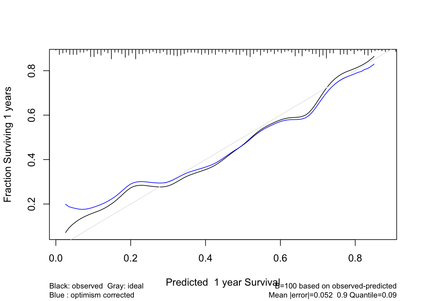
- Plot the shape of the effect of each predictor on the linear predictor
- All effects centered: can be placed on common scale
- LR \(\chi^2\) statistics, penalized for d.f., plotted in descending order
Code
ggplot(Predict(f, ref.zero=TRUE), vnames='names', anova=a)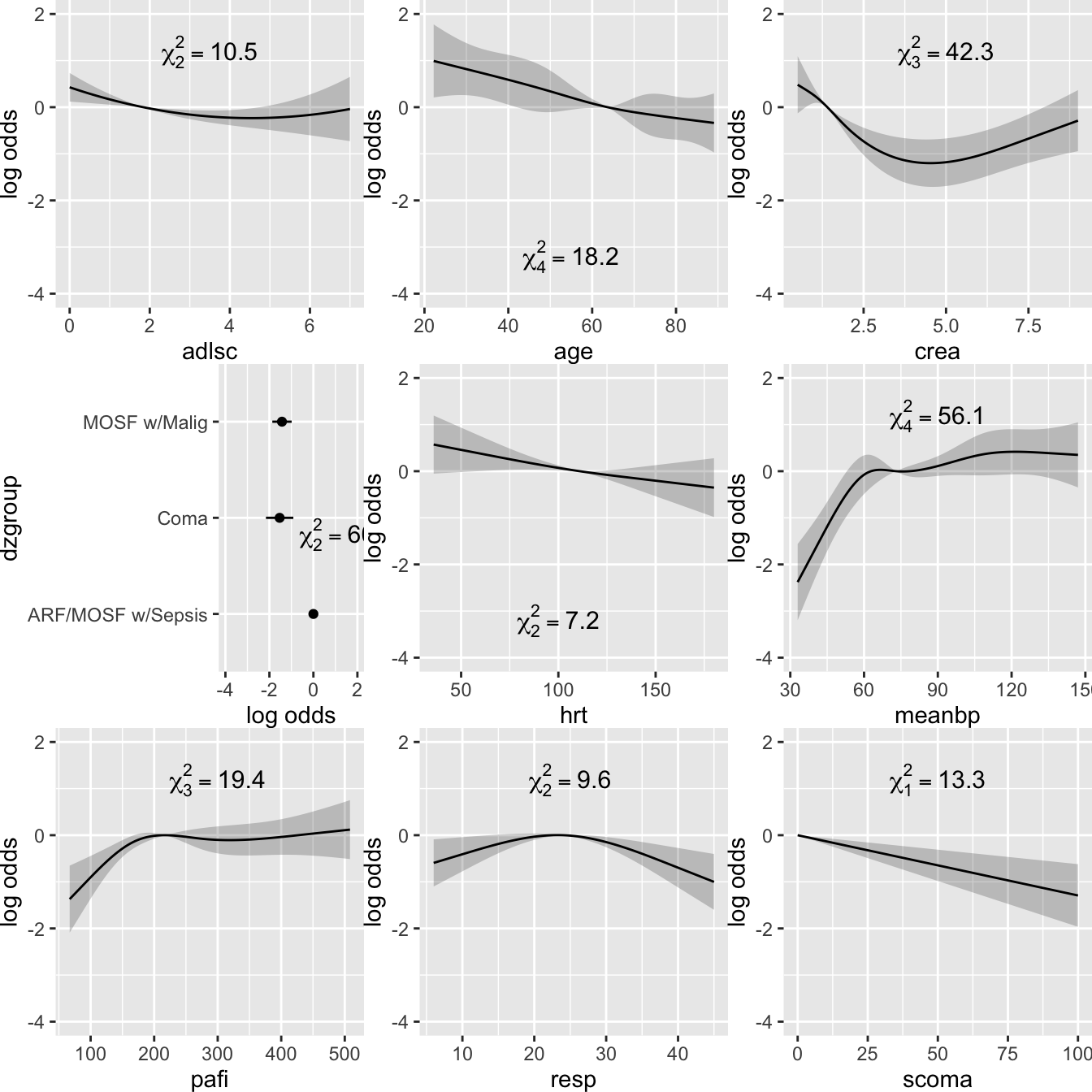
Convert the \(y\)-axis to show instead the predicted proportion of a 4y follow-up in which the patient is alive.
Code
ggplot(Predict(f, fun=Prop4y), vnames='names')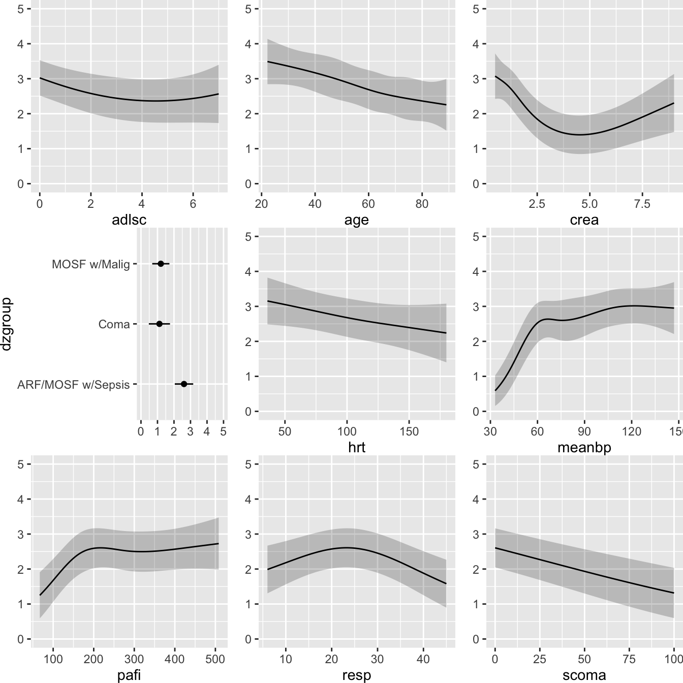
Compute Wald confidence intervals of age 40:60 odds ratios two different ways, and the corresponding more accurate profile likelihood interval. A likelihood ratio test for the one degree of freedom contrast between ages 40 and 60 is also included. This is a focused contrast in comparison with the overall 4 degree of freedom chunk LR test for age.
Code
summary(f, age=c(40, 60), est.all=FALSE)Effects Response: Y |
|||||||
| Low | High | Δ | Effect | S.E. | Lower 0.95 | Upper 0.95 | |
|---|---|---|---|---|---|---|---|
| age | 40 | 60 | 20 | -0.5075 | 0.2572 | -1.0120 | -0.003335 |
| Odds Ratio | 40 | 60 | 20 | 0.6020 | 0.3636 | 0.996700 | |
Code
k <- contrast(f, list(age=60), list(age=40))
print(k, fun=exp)
dzgroup meanbp crea hrt scoma pafi adlsc resp Contrast
1 ARF/MOSF w/Sepsis 73 1.399902 111 0 217.5 1.839 24 0.6019899
Lower Upper Z Pr(>|z|)
1 0.3636024 0.9966706 -1.97 0.0485
Confidence intervals are 0.95 individual intervalsCode
k <- contrast(f, list(age=60), list(age=40), conf.type='profile')
print(k, fun=exp)
dzgroup meanbp crea hrt scoma pafi adlsc resp Contrast
1 ARF/MOSF w/Sepsis 73 1.399902 111 0 217.5 1.839 24 0.6019899
Lower Upper Χ² Pr(>Χ²)
1 0.3629426 0.9955884 3.91 0.048
Confidence intervals are 0.95 profile likelihood intervalsCompute estimated survival curves and point wise 0.95 confidence bands for several covariate combinations.
Code
survplot(f, dzgroup, meanbp=c(40, 100), crea=c(1, 1.4, 2.5), conf.int=0.95)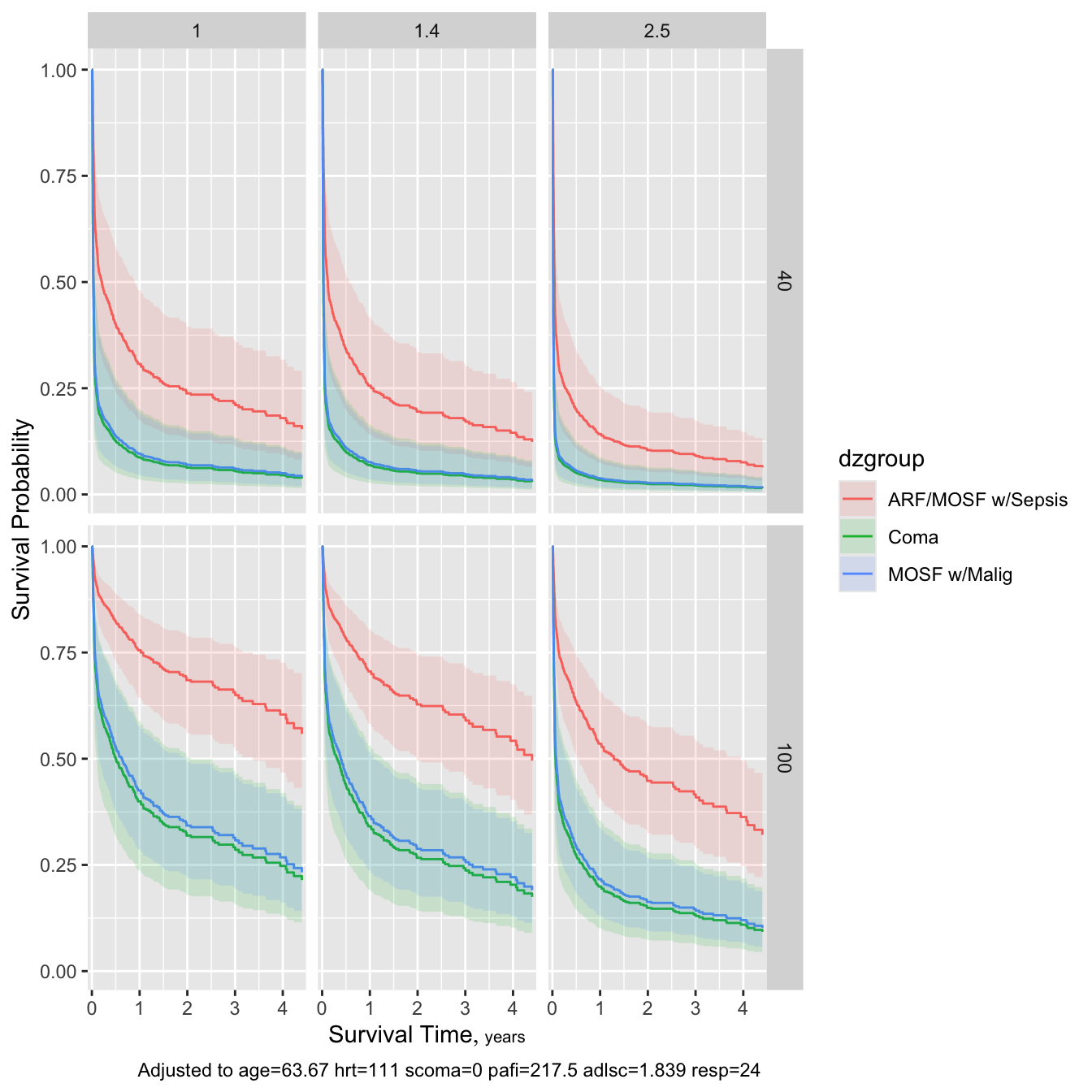
25.9.1 Strong Internal Validation of the Fitted Model Using the Bootstrap
Validate indexes describing the fitted model using the optimism bootstrap.
Code
# First add data to model fit so bootstrap can re-sample
#  from the data
set.seed(717)
validate(f, B=300)| Index | Original Sample |
Training Sample |
Test Sample |
Optimism | Corrected Index |
Lower | Upper | Successful Resamples |
|---|---|---|---|---|---|---|---|---|
| Dxy | 0.4818 | 0.4997 | 0.4634 | 0.0363 | 0.4454 | 0.3944 | 0.4974 | 300 |
| R2 | 0.404 | 0.4312 | 0.3781 | 0.0531 | 0.3509 | 0.2882 | 0.4169 | 300 |
| Slope | 1 | 1 | 0.8797 | 0.1203 | 0.8797 | 0.7251 | 1.0407 | 300 |
| g | 1.6756 | 1.7988 | 1.5824 | 0.2165 | 1.4591 | 1.1896 | 1.7054 | 300 |
| Mean |Pr(Y≥Y0.5)-0.5| | 0.2656 | 0.2745 | 0.2591 | 0.0154 | 0.2502 | 0.2289 | 0.2721 | 300 |
Validate a calibration curve for 1-time unit survival predictions using the optimism bootstrap incorporating smoothed moving overlapping window Kaplan-Meier estimates. Also use the adaptive linear spline hare method. Usually hare does too much smoothing.
Code
# Default is method='smoothkm' with eps=30 (30 observations in each moving window)
set.seed(3)
cal1 <- calibrate(f, B=100, u=1) #, val.surv.args=list(method='smoothkm', eps=30))
plot(cal1)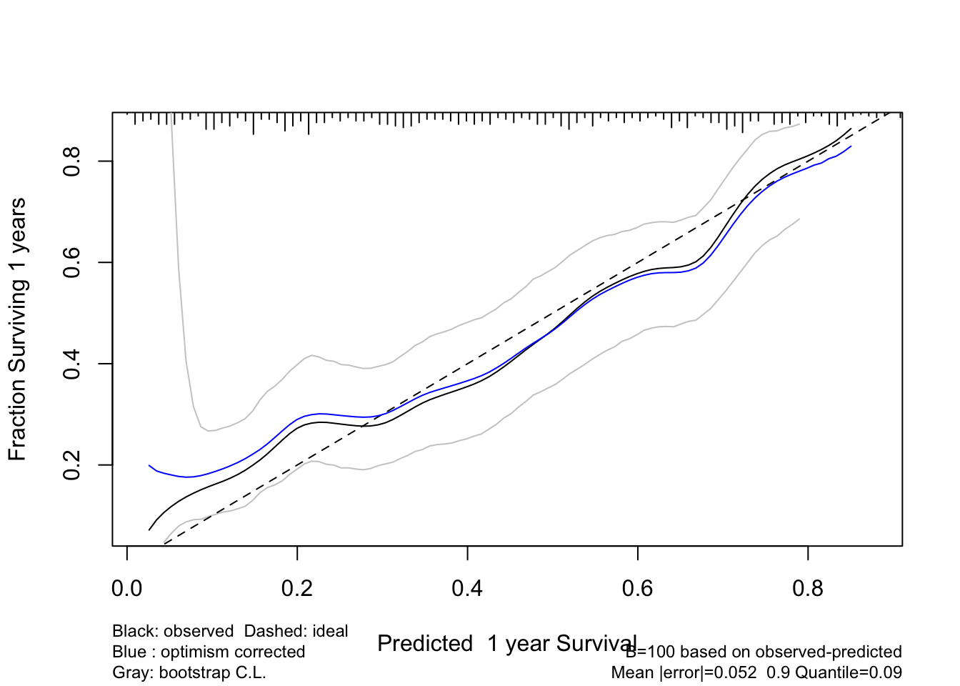
Code
cal2 <- calibrate(f, B=100, u=1, val.surv.args=list(method='hare'))
plot(cal2)