```{r include=FALSE}
options(qproject='rms', prType='html')
require(Hmisc)
require(qreport)
getRs('qbookfun.r')
hookaddcap()
knitr::set_alias(w = 'fig.width', h = 'fig.height', cap = 'fig.cap', scap ='fig.scap')
```
# Describing, Resampling, Validating, and Simplifying the Model {#sec-val}
## Describing the Fitted Model {#sec-val-describe-model}
`r mrg(sound("v-1"))`
### Interpreting Effects
<!-- NEW: predictions plot below -->
* Regression coefficients if 1 d.f. per factor, no interaction `r ipacue()`
* **Not** standardized regression coefficients
* Many programs print meaningless estimates such as effect of
increasing age$^2$ by one unit, holding age constant
* Need to account for nonlinearity, interaction, and use meaningful
ranges
* For monotonic relationships, estimate $X\hat{\beta}$ at
quartiles of continuous variables, separately for various
levels of interacting factors
* Subtract estimates, anti-log, e.g., to get inter-quartile-range `r ipacue()`
odds or hazards ratios. Base C.L. on s.e. of difference. See @fig-coxcase-summary.
* Partial effect plot: Plot effect of each predictor on $X\beta$ or some transformation. See @fig-coxcase-shapes.
See also @kar09vis. Fox and Weisberg have [other excellent approaches](https://cran.r-project.org/web/packages/effects/vignettes/predictor-effects-gallery.pdf) to displaying predictor effects
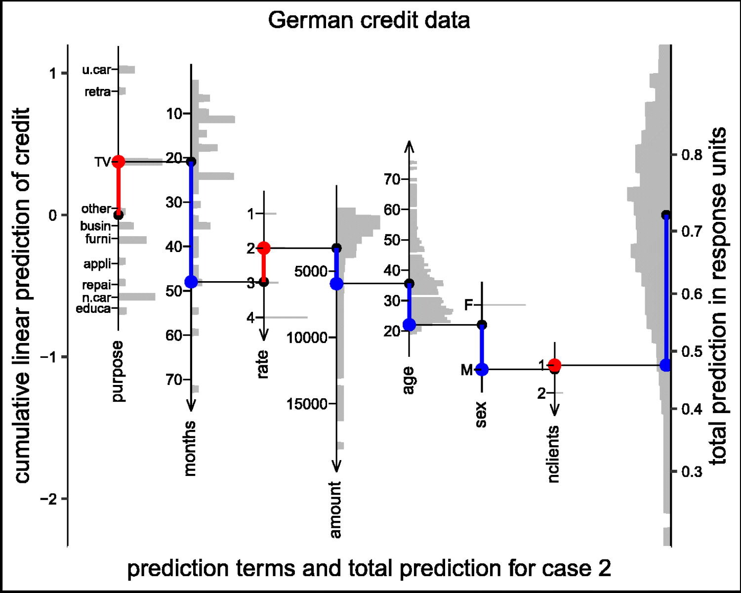
* [Predictions plot](https://www.tandfonline.com/doi/full/10.1080/00031305.2025.2539235) of Peter Rousseeuw
* Nomogram. See @fig-coxcase-nomogram
* Use regression tree to approximate the full model
<img src="images/predictions_plot.jpg" width="100%">
Predictions plot from Rousseeuw (2026)
#### Contrasts {#sec-val-contrast}
Forming contrasts through differences in predicted values is the most general and easy way to estimate effects of interest in a model. This is because
* One needs only to specify two or more sets of predictor settings to contrast
* Predictor coding, nonlinear terms, and interactions are automatically taken into account
* Unspecified predictors can default to reference values such as medians for continuous predictors and modes for categorical ones. The values used for unspecified predictors only matter if they interact with predictors that are changing in the contrast.
* Approximate methods are available for getting simultaneous confidence intervals over a whole sequence of contrasts (e.g., simultaneous confidence bands for an entire range of ages) when contrasts produce more than one estimate
* The approach extends to any order of differences. E.g., interaction contrasts are formed with double differences.
* Contrasts allow assessment of linearity over a given predictor range in a spline fit
* Contrasts allow assessment of "partial interactions", i.e., whether there is an interaction between one predictor and a subset of the levels of another predictor
* The R `predict` function provides the $X$ (design matrix) that goes along with each requested prediction, and simple matrix algebra provides needed covariance matrices once differences in design matrices are formed
On the latter point, a single difference contrast such as one comparing 30 year old males with 40 year old males would generate two design matrices $X_{1}, X_{2}$, and the contrast
$X_{1}\beta - X_{2}\beta = (X_{1} - X_{2})\beta$.
Consider a series of examples in which predicted values from a fitted model are symbolized by a function $f$ of the predictor settings, with continuous predictors $A$ and $B$ and a categorical predictor $C$ with levels $i, j, k$. Let the reference (detault) values of the predictors be $a$ (median of $A$), $b$ (median of $B$), and $c$ (modal (most frequent) category of $C$). [The term "average slope" used below will be **the** slope if the predictor has a linear effect, otherwise it is the average slope over the indicated interval. See [here](https://stats.stackexchange.com/questions/639430) for more information.]{.aside}
##### Single Difference Contrasts
* Average slope of $A$ over $A \in [1, 2]$: $f(2, b, c) - f(1, b, c)$
* Difference between categories $j$ and $k$ in $C$: $f(a, b, j) - f(a, b, k)$
* Effect of an entire range of predictor values against a single reference value: $f(1:10, b, c) - f(5, b, c)$ (a simultaneous confidence band would be useful here)
##### Double Difference Contrasts
* Linearity in $A$ over $A \in [1, 3]$: $f(3, b, c) - f(2, b, c) - [f(2, b, c) - f(1, b, c)] = f(3, b, c) - 2f(2, b, c) + f(1, b, c)$
* Interaction between $A$ and $C$ with respect to only two levels of $C$: $f(2, b, j) - f(1, b, j) - [f(2, b, k) - f(1, b, k)]$
* Interaction between $A$ and $B$ when $A$ varies from 1 to 3 and $B$ varies from 5 to 6: $f(3, 5, c) - f(1, 5, c) - [f(3, 6, c) - f(1, 6, c)]$
* Effect of $C=i$ vs. $C=j$ over a regular grid of values of $B$: $f(a, 5:15, i) - f(a, 5:15, j)$ (with possible simultaneous band; this is often a better way of getting hazard ratios in a Cox proportional hazards model, as the user has control of the reference value)
##### Triple Difference Contrasts
* Third-order interactions
* Assessment of nonlinearity in the $A\times B$ interaction (differences in double differences)
The R `rms` package [`contrast` function](https://www.rdocumentation.org/packages/rms/versions/6.7-1/topics/contrast.rms) (full name `contrast.rms`) provides predicted values, differences, and double difference contrasts. The latter is specified by providing four lists of predictor settings.
### Indexes of Model Performance {#sec-val-index}
`r mrg(sound("v-2"))`
#### Error Measures
* Central tendency of prediction errors `r ipacue()`
+ Mean absolute prediction error: mean $|Y - \hat{Y}|$
+ Mean squared prediction error
- Binary $Y$: Brier score (quadratic proper scoring rule)
+ Logarithmic proper scoring rule (avg. log-likelihood)
* Discrimination measures `r ipacue()`
+ Pure discrimination: rank correlation of $(\hat{Y}, Y)$
- Spearman $\rho$, Kendall $\tau$, Somers' $D_{xy}$
- $Y$ binary $\rightarrow$ $D_{xy} = 2\times (C -
\frac{1}{2})$ <br> $C$ = concordance probability = area under
receiver operating characteristic curve $\propto$
Wilcoxon-Mann-Whitney statistic
+ Mostly discrimination: $R^{2}$
- $R^{2}_{\mathrm{adj}}$---overfitting corrected if model pre-specified
+ Brier score can be decomposed into discrimination and
calibration components
+ Discrimination measures based on variation in $\hat{Y}$
- regression sum of squares
- $g$--index
- see [here](https://fharrell.com/post/addvalue) for related information
* Calibration measures `r ipacue()`
+ calibration--in--the--large: average $\hat{Y}$ vs. average $Y$
+ high-resolution calibration curve (calibration--in--the--small). See @fig-titanic-calibrate.
+ calibration slope and intercept
+ maximum absolute calibration error
+ mean absolute calibration error
+ 0.9 quantile of calibration error
See @cal16cal for a nice discussion of
different levels of calibration stringency and their relationship to
likelihood of errors in decision making.
**$g$--Index**
`r mrg(sound("v-3"))`
* Based on Gini's mean difference `r ipacue()`
+ mean over all possible $i \neq j$ of $|Z_{i} - Z_{j}|$
+ interpretable, robust, highly efficient measure of variation
* $g =$ Gini's mean difference of $X_{i}\hat{\beta} = \hat{Y}$
* Example: $Y=$ systolic blood pressure; $g = 11$mmHg is typical
difference in $\hat{Y}$
* Independent of censoring etc.
* For models in which anti-log of difference in $\hat{Y}$ `r ipacue()`
represent meaningful ratios (odds ratios, hazard ratios, ratio of
medians):<br> $g_{r} = \exp(g)$
* For models in which $\hat{Y}$ can be turned into a probability
estimate (e.g., logistic regression):<br> $g_{p} =$ Gini's mean
difference of $\hat{P}$
* These $g$--indexes represent e.g. "typical" odds ratios, "typical"
risk differences
* Can define partial $g$
<!-- NEW 2023-09-16 -->
### Relative Explained Variation {#sec-val-rev}
* In OLS linear models $R^2$ is an excellent measure of explained variation in $Y$
* Fraction of variance of $Y$ that is explained by $X$
* SSR = $\sum_{i=1}^{n} (\hat{Y}_{i} - \bar{\hat{Y}})^2$ = regression sum of squares
+ proportional to variance of $\hat{Y}$
* SSE = $\sum_{i=1}^{n} (Y_{i} - \hat{Y}_{i})^2$ = error sum of squares = residual sum of squares
+ proportional to error variance
* SST = $\sum_{i=1}^{n} (Y_{i} - \bar{Y})^2$ = total sum of squares
+ proportion to variance of $Y$
* SST = SSR + SSE
* $R^{2} =$ SSR/SST = 1 - SSE/SST
* For each part of the model can compute its partial SSR = loss in SSR after refitting the model upon removing the part of the model being assessed
* Partial $R^{2}$ = (partial SSR)/SST
* Relative partial $R^{2} = \frac{\text{partial } R^{2}}{R^{2}} =$ partial SSR divided by full model SSR
* Relative partial $R^{2}$ = portion of **explainable** (by $X$) variation in $Y$ that is explained by one or more terms in the model
* Relative explained variation: REV
* REVs do not need to sum to 1.0
+ collinearities
+ computing REVs for overlapping model terms
* When a predictor interacts with another predictor, the predictor's REV is taken from the combined predictive information in
+ the predictor main effect (including any nonlinear terms)
+ any interaction terms involving that effect
#### Extension to Other Models
* For models fitted using maximum likelihood estimation, can compute the partial likelihood ratio $\chi^2$ statistic for each set and divide that by the total model LR $\chi^2$
* See also @sec-mle and the example below
* This is an excellent measure but requires more computation and doesn't extend to models not having a likelihood or to Bayesian modeling
* Need a general purpose REV measure that works on virtually all models using all estimation techniques
* Letting $\hat{Y} = X\hat{\beta}$ be the estimated linear predictor from the model
* Use the same design matrix $X$ used to get $\hat{Y}$
* Predict $\hat{Y}$ from $X$ using OLS
* The $R^{2}$ from this model is 1.0
* SSE = 0; ignore this and take variance-covariance matrix as $(X'X)^{-1}$ since SSR is used only on a relative basis
* REV = $\frac{\text{partial SSR }}{\text{SSR}}$
* Identical to relative $R^2$ if original model was OLS
* Easily lends itself to uncertainty intervals
+ frequentist: bootstrap the original model fit and save the repeated coefficient estimates (done by R `rms` package `bootcov` function); compute bootstrap confidence intervals for REVs; see @sec-val-boot and example below
+ Bayesian: compute REV for each posterior draw of $\beta$ and from the repeated REVs compute highest posterior density uncertainty intervals
* Implemented in R `rms` package [`rexVar` function](https://github.com/harrelfe/rms/blob/master/R/rexVar.r)
See @luc14rel for a nice review of log-likelihood-based relative importance measures.
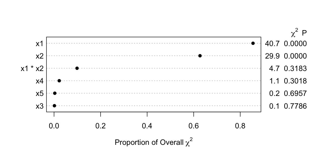
#### Example
* Ordinal regression model (proportional odds model for continuous Y)
* Allow for quadratic effects for two predictors which are allowed to interact
* Three other predictors that are irrelevant are modeled linearly
* Bootstrap
* Through uncertainty intervals for REVs show that when the sample size is inadequate for fitting an accurate reproducible model it's also inadequate for measuring variable importance
```{r}
require(rms)
options(prType='html') #<1>
n <- 60
set.seed(3)
x1 <- rnorm(n)
x2 <- rnorm(n)
x3 <- rnorm(n)
x4 <- rnorm(n)
x5 <- rnorm(n)
y <- round(x1 + x2 + rnorm(n), 2)
d <- data.frame(x1, x2, x3, x4, y)
f <- orm(y ~ pol(x1, 2) * pol(x2, 2) + x3 + x4 + x5,
x=TRUE, y=TRUE) #<2>
a <- anova(f, test='LR') #<3>
a
```
1. Makes `print` methods output html for prettier printing
2. `x=TRUE, y=TRUE` are needed for later bootstrapping
3. Computes likelihood ratio $\chi^2$ test statistics for all partial effects in the model plus for the whole model
```{r}
#| label: fig-val-lr
#| fig-cap: Relative LR $\chi^2$ explained. Interaction effects are added to main effects.
#| fig-height: 3.5
plot(a, what='proportion chisq', sort='ascending') #<1>
```
1. Plots ratios of partial $\chi^2$ to total model LR $\chi^2$. `ascending` is really a misnomer.
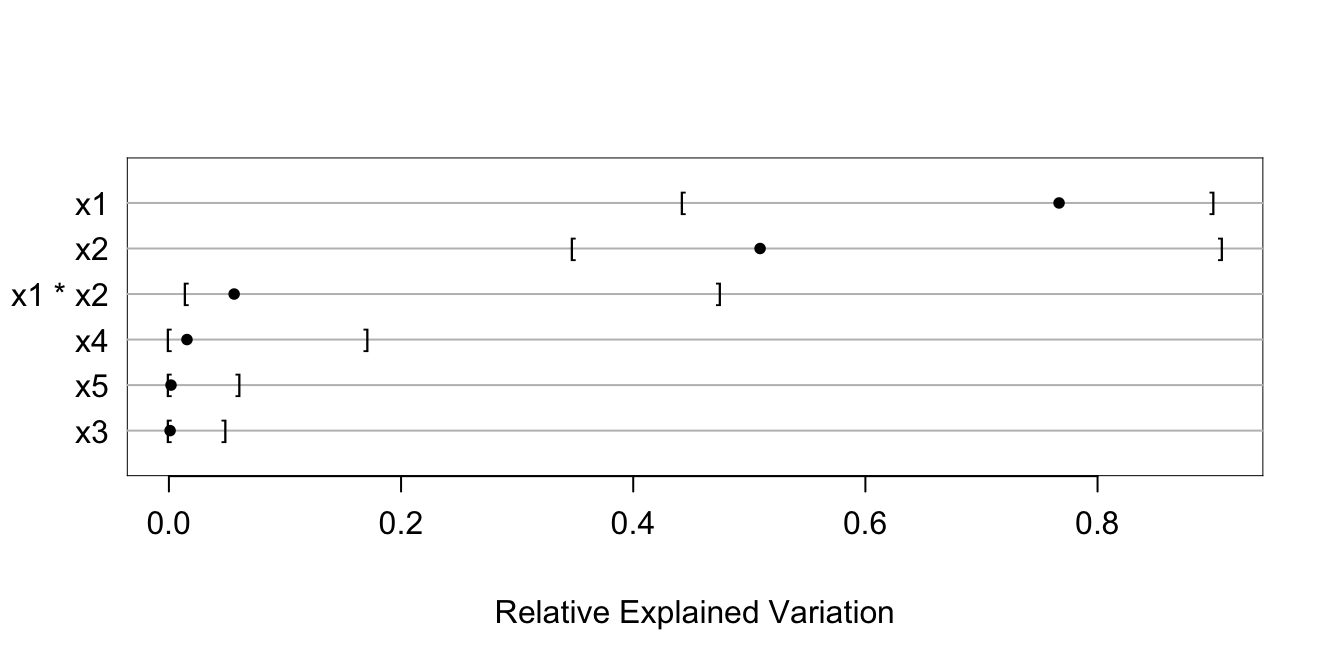
Let's use the bootstrap to get uncertainty intervals for relative explained variation. Note that for this small sample size, bootstrap parameter estimates are highly unstable and have standard errors that are about $4\times$ larger than the estimates from maximum likelihood estimation. We tell `bootcov` to only retain intercepts that target the median of `y`.
```{r}
#| label: fig-val-rex
#| fig-cap: Relative explained variation due to each predictor. Interaction effects are added to main effects. Intervals are 0.95 bootstrap percentile confidence intervals.
#| fig-height: 3.5
# Have bootcov save only one intercept for each fit: the one corresponding to the
# median of y
g <- bootcov(f, B=300, ytarget=NA)
rx <- rexVar(g, data=d)
rx
plot(rx)
```
## The Bootstrap {#sec-val-boot}
`r mrg(sound("v-4"))`
* If know population model, use simulation or analytic derivations `r ipacue()`
to study behavior of statistical estimator
* Suppose $Y$ has a cumulative dist. fctn. $F(y) = \Pr\{Y \leq y\}$
* We have sample of size $n$ from $F(y)$, <br>
$Y_{1}, Y_{2}, \ldots, Y_{n}$
* Steps:
1. Repeatedly simulate sample of size $n$ from $F$
1. Compute statistic of interest
1. Study behavior over $B$ repetitions
* Example: 1000 samples, 1000 sample medians, compute their sample
variance `r ipacue()`
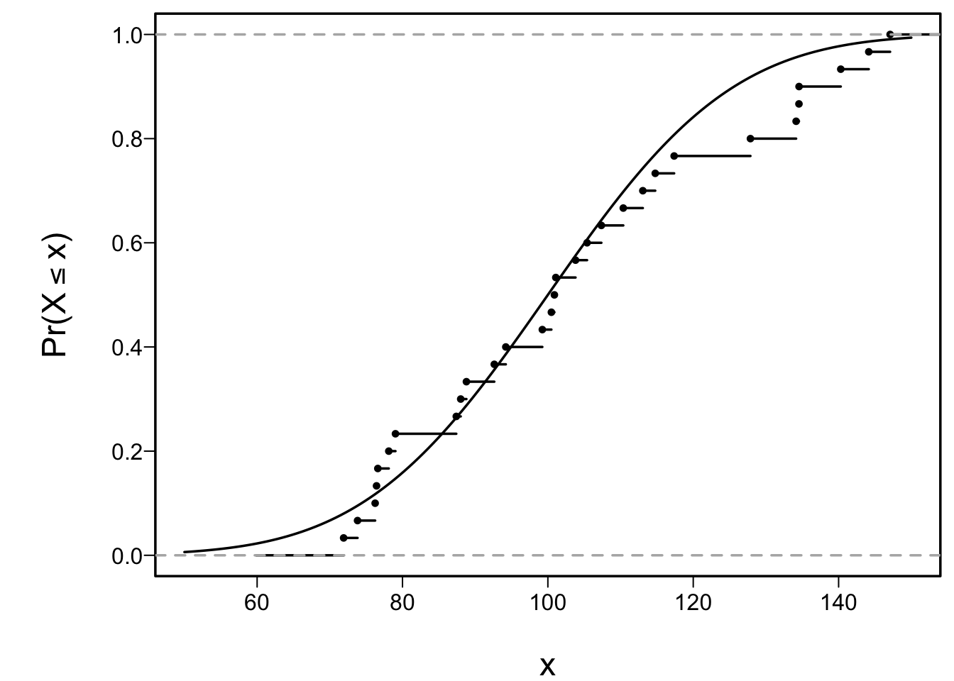
* $F$ unknown $\rightarrow$ estimate by empirical dist. fctn.
$$
F_{n}(y) = \frac{1}{n}\sum_{i=1}^{n} [Y_{i} \leq y].
$$
* Example: sample of size $n=30$ from a normal distribution with
mean 100 and SD 10
```{r cap='Empirical and population cumulative distribution function'}
#| label: fig-val-cdf
spar()
set.seed(6)
x <- rnorm(30, 100, 20)
xs <- seq(50, 150, length=150)
cdf <- pnorm(xs, 100, 20)
plot(xs, cdf, type='l', ylim=c(0,1),
     xlab=expression(x),
     ylab=expression(paste("Pr(", X <= x, ")")))
lines(ecdf(x), cex=.5)
```
* $F_{n}$ corresponds to density function placing probability `r ipacue()`
$\frac{1}{n}$ at each observed data point ($\frac{k}{n}$ if
point duplicated $k$ times)
* Pretend that $F \equiv F_{n}$
* Sampling from $F_{n} \equiv$ sampling with replacement from
observed data $Y_{1},\ldots,Y_{n}$
* Large $n$ $\rightarrow$ selects $1-e^{-1} \approx 0.632$ of original data points
in each bootstrap sample at least once
* Some observations not selected, others selected more than once
* Efron's _bootstrap_ $\rightarrow$ `r ipacue()`
general-purpose technique for estimating properties of estimators
without assuming or knowing distribution of data $F$
* Take $B$ samples of size $n$ with replacement, choose $B$ `r ipacue()`
so that summary measure of individual statistics $\approx$
summary if $B=\infty$
* Bootstrap based on distribution of
_observed_ differences between a resampled parameter estimate
and the original estimate telling us about the distribution of
_unobservable_ differences between the original estimate and the
unknown parameter
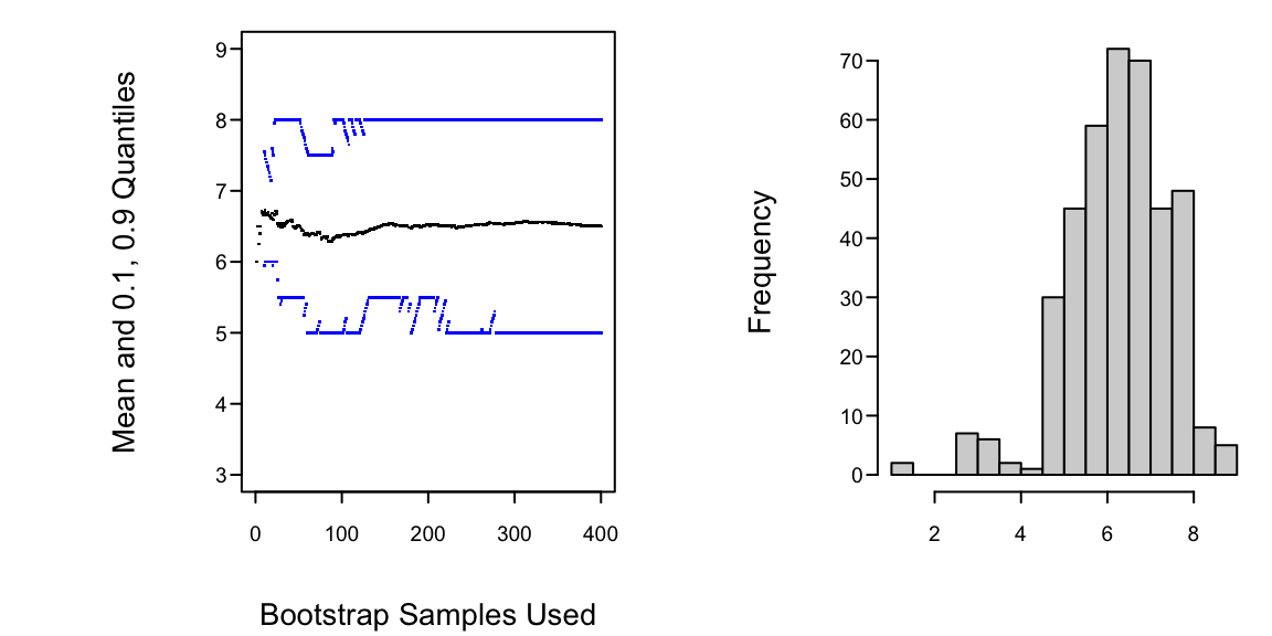
Example: Data $(1,5,6,7,8,9)$, obtain 0.80 confidence interval for `r ipacue()`
population median, and estimate of population expected value
of sample median (only to estimate the bias in the original
estimate of the median).
<!-- In 1st edition used .Random.seed <- c(1,11,4,9,61,2,29,53,34,4,16,3)--->
```{r h=3, w=6, cap='Estimating properties of sample median using the bootstrap'}
#| label: fig-val-boot
spar(ps=9, mfrow=c(1,2))
options(digits=3)
y <- c(2,5,6,7,8,9,10,11,12,13,14,19,20,21)
y <- c(1,5,6,7,8,9)
set.seed(17)
n   <- length(y)
n2  <- n/2
n21 <- n2+1
B   <- 400
M <- double(B)
plot(0, 0, xlim=c(0,B), ylim=c(3,9),
     xlab="Bootstrap Samples Used",
     ylab="Mean and 0.1, 0.9 Quantiles", type="n")
for(i in 1:B) {
  s <- sample(1:n, n, replace=T)
  x <- sort(y[s])
  m <- .5*(x[n2]+x[n21])
  M[i] <- m
  points(i, mean(M[1:i]), pch=46)
  if(i>=10) {
    q <- quantile(M[1:i], c(.1,.9))
    points(i, q[1], pch=46, col='blue')
    points(i, q[2], pch=46, col='blue')
  }
}
table(M)
hist(M, nclass=length(unique(M)), xlab="", main="")
```
First 20 samples:
| Bootstrap Sample | | Sample Median |
|-----|-----|-----|
| 1 5 5 7 8 9 | | 6.0 |
| 1 1 5 7 9 9 | | 6.0 |
| 6 7 7 8 9 9 | | 7.5 |
| 1 1 5 6 8 9 | | 5.5 |
| 1 6 7 7 8 8 | | 7.0 |
| 1 5 6 8 8 9 | | 7.0 |
| 1 6 8 8 9 9 | | 8.0 |
| 5 5 6 7 8 9 | | 6.5 |
| 1 5 6 7 7 8 | | 6.5 |
| 1 5 6 8 9 9 | | 7.0 |
| 1 5 7 7 8 9 | | 7.0 |
| 1 5 6 6 7 8 | | 6.0 |
| 1 6 6 7 8 9 | | 6.5 |
| 5 6 7 7 8 9 | | 7.0 |
| 1 5 6 8 8 8 | | 7.0 |
| 1 1 6 6 7 8 | | 6.0 |
| 5 5 5 8 8 9 | | 6.5 |
| 5 6 6 6 7 7 | | 6.0 |
| 1 5 7 9 9 9 | | 8.0 |
| 1 1 5 5 5 7 | | 5.0 |
* Histogram tells us whether we can assume normality for the bootstrap `r ipacue()`
medians or need to use quantiles of medians to construct C.L.
* Need high $B$ for quantiles, low for variance (but see @boo98mon)
* See @efr20aut for useful information about bootstrap
confidence intervals and the latest `R` functions
## Model Validation {#sec-val-validation}
### Introduction
`r mrg(sound("v-5"))`
* External validation (best: another country at another time); `r ipacue()`
also validates sampling, measurements\footnote{But in many cases it
is better to combine data and include country or calendar time as
a predictor.}
* Internal
+ apparent (evaluate fit on same data used to create fit)
+ data splitting
+ cross-validation
+ bootstrap: get overfitting-corrected accuracy index
* Best way to make model fit data well is to discard much of the data `r ipacue()` (not recommended!)
* Predictions on another dataset will be inaccurate
* Need unbiased assessment of predictive accuracy
**Working definition of external validation**: Validation of a
prediction tool on a sample that was not available at publication
time.
**Alternate**: Validation of a prediction tool by an
independent research team.
One suggested hierarchy of the quality of various validation methods
is as follows, ordered from worst to best.
1. Attempting several validations (internal or external) and `r ipacue()`
reporting only the one that "worked"
1. Reporting apparent performance on the training dataset (no validation)
1. Reporting predictive accuracy on an undersized independent test sample
1. Internal validation using data splitting where at least one of
the training and test samples is not huge and the investigator is
not aware of the arbitrariness of variable selection done on a
single sample
1. Strong internal validation using 100 repeats of 10-fold `r ipacue()`
cross-validation or several hundred bootstrap resamples, repeating
_all_ analysis steps involving $Y$ afresh at each re-sample and
the arbitrariness of selected "important variables" is reported
(if variable selection is used)
1. External validation on a large test sample, done by the original
research team
1. Re-analysis by an independent research team using strong
internal validation of the original dataset
1. External validation using new test data, done by an independent
research team
1. External validation using new test data generated using
different instruments/technology, done by an independent research team
Some points to consider:
* Unless both sample sizes are huge, external validation can be `r ipacue()`
low precision
* External validation can be costly and slow and may result in
disappointment that would have been revealed earlier with rigorous
internal validation
* External validation is sometimes _gamed_; researchers
disappointed in the validation sometimes ask for a "do over";
resampling validation is harder to game as long as all analytical
steps using $Y$ are repeated each time.
* Instead of external validation to determine model applicability `r ipacue()`
at a different time or place, and being disappointed if the model
does not work in that setting, consider building a
unified model containing time and place as predictors
* When the model was fully pre-specified, external validation
tests _the model_
* But when the model was fitted using machine learning, feature
screening, variable selection, or model selection, the model developed
using training data is usually only an example of a model, and the
test sample validation could be called an _example validation_
* When resampling is used to repeat _all_ modeling steps for
each resample, rigorous internal validation tests the _process_
used to develop the model and happens to also provide a
high-precision estimate of the likely future performance of the
"final" model developed using that process, properly penalizing
for model uncertainty.
* Resampling also reveals the volatility of the model selection process
$\rightarrow$ See [BBR](http://hbiostat.org/bbr/reg.html#internal-vs.-external-model-validation)
@col16sam estimate that a typical sample size
needed for externally validating a time-to-event model is 200 events. @ril24evaa has more in-depth guidance for sizing an external validation study.
### Which Quantities Should Be Used in Validation? {#sec-val-which}
`r mrg(sound("v-6"))`
* OLS: $R^2$ is one good measure for quantifying drop-off in `r ipacue()`
predictive ability
* Example: $n=10, p=9$, apparent $R^{2}=1$ but $R^2$ will be close
to zero on new subjects
* Example: $n=20, p=10$, apparent $R^{2}=.9$, $R^2$ on new data
0.7, $R^{2}_{adj} = 0.79$
* Adjusted $R^2$ solves much of the bias problem assuming $p$ in
its formula is the largest number of parameters ever examined against $Y$
* Few other adjusted indexes exist
* Also need to validate models with phantom d.f.
* Cross-validation or bootstrap can provide unbiased estimate of `r ipacue()`
any index; bootstrap has higher precision
* Two main types of quantities to validate
1. Calibration or reliability: ability to make unbiased estimates
of response ($\hat{Y}$ vs. $Y$)
1. Discrimination: ability to separate responses <br>
OLS: $R^2$; $g$-index; binary logistic model: ROC area, equivalent
to rank correlation between predicted probability of event and 0/1 event
* Unbiased validation nearly always necessary, to detect overfitting
### Data-Splitting {#sec-val-split}
`r mrg(sound("v-7"))`
* Split data into _training_ and _test_ sets `r ipacue()`
* Interesting to compare index of accuracy in training and test
* Freeze parameters from training
* Make sure you allow $R^{2} = 1-SSE/SST$ for test sample to be
$<0$
* Don't compute ordinary $R^2$ on $X\hat{\beta}$ vs. $Y$; this
allows for linear recalibration $aX\hat{\beta} + b$ vs. $Y$
* Test sample must be large enough to obtain very accurate
assessment of accuracy `r ipacue()`
* Training sample is what's left
* Example: overall sample $n=300$, training sample $n=200$,
develop model, freeze $\hat{\beta}$, predict on test sample
($n=100$), $R^{2} = 1 -
\frac{\sum(Y_{i}-X_{i}\hat{\beta})^{2}}{\sum(Y_{i}-\bar{Y})^{2}}$.
* Disadvantages of data splitting: `r ipacue()`
1. Costly in $\downarrow n$ [@roe91pre; @bre92lit]
1. Requires _decision_ to split at beginning of analysis
1. Requires larger sample held out than cross-validation
1. Results vary if split again
1. Does not validate the final model (from recombined data)
1. Not helpful in getting CL corrected for var. selection
1. Nice summary of disadvantages: @ste18val
### Improvements on Data-Splitting: Resampling {#sec-val-resampling}
`r mrg(sound("v-8"))`
<!-- ?? TODO 3rd bullet ref pg:lrm-sw5p -->
* No sacrifice in sample size `r ipacue()`
* Work when modeling process automated
* Bootstrap excellent for studying arbitrariness of variable
selection [@sau92boo].
* Cross-validation solves many problems of data
splitting [@hou90pre; @sha93lin; @wu86jac; @efr83est]
* Example of $\times$-validation: `r ipacue()`
1. Split data at random into 10 tenths
1. Leave out $\frac{1}{10}$ of data at a time
1. Develop model on $\frac{9}{10}$, including any
variable selection, pre-testing, etc.
1. Freeze coefficients, evaluate on $\frac{1}{10}$
1. Average $R^2$ over 10 reps
* Drawbacks:
1. Choice of number of groups and repetitions
1. Doesn't show full variability of var. selection
1. Does not validate full model
1. Lower precision than bootstrap
1. Need to do 50 repeats of 10-fold cross-validation to
ensure adequate precision
* Randomization method `r ipacue()`
1. Randomly permute $Y$
1. Optimism = performance of fitted model compared to
what expect by chance
### Validation Using the Bootstrap {#sec-val-bootval}
`r mrg(sound("v-9"))`
* Estimate optimism of _final whole sample fit_ without `r ipacue()`
holding out data
* From original $X$ and $Y$ select sample of size $n$ with replacement
* Derive model from bootstrap sample
* Apply to original sample
* Simple bootstrap uses average of indexes computed on original
sample
* Estimated optimism = difference in indexes
* Repeat about $B=100$ times, get average expected optimism
* Subtract average optimism from apparent index in final model
* Example: $n=1000$, have developed a final model that is `r ipacue()`
hopefully ready to publish. Call estimates from this final model
$\hat{\beta}$.
+ final model has apparent $R^2$ ($R^{2}_{app}$) =0.4
+ how inflated is $R^{2}_{app}$?
+ get resamples of size 1000 with replacement from original 1000
+ for each resample compute $R^{2}_{boot}$ = apparent $R^2$ in
bootstrap sample
+ freeze these coefficients (call them $\hat{\beta}_{boot}$),
apply to original (whole) sample $(X_{orig}, Y_{orig})$ to
get $R^{2}_{orig} = R^{2}(X_{orig}\hat{\beta}_{boot}, Y_{orig})$
+ optimism = $R^{2}_{boot} - R^{2}_{orig}$
+ average over $B=100$ optimisms to get $\overline{optimism}$
+ $R^{2}_{overfitting~corrected} = R^{2}_{app} - \overline{optimism}$
<!-- ?? TODO first bullet ref pg:lrm-sex-age-response-boot -->
* Example: Chapter 8
* Is estimating unconditional (not conditional on $X$) distribution `r ipacue()`
of $R^2$, etc. [@far92cos, p. 217]
* Conditional estimates would require assuming the model one is trying
to validate
* Efron's "$.632$" method may perform better (reduce bias further)
for small $n$ [@efr83est], [@efr93int, p. 253], @efr97imp
Bootstrap useful for assessing calibration in addition to discrimination:
`r mrg(sound("v-10"))`
* Fit $C(Y|X) = X\beta$ on bootstrap sample `r ipacue()`
* Re-fit $C(Y|X) = \gamma_{0} + \gamma_{1}X\hat{\beta}$ on same data
* $\hat{\gamma}_{0}=0, \hat{\gamma}_{1}=1$
* Test data (original dataset): re-estimate $\gamma_{0}, \gamma_{1}$
* $\hat{\gamma}_{1}<1$ if overfit,
$\hat{\gamma}_{0} > 0$ to compensate
* $\hat{\gamma}_{1}$ quantifies overfitting and useful for improving
calibration [@spi86pro]
* Use Efron's method to estimate optimism in $(0,1)$, estimate
$(\gamma_{0}, \gamma_{1})$ by subtracting optimism from $(0,1)$
* See also @cop87cro and @hou90pre, p. 1318
See @fre88imp for warnings about the bootstrap, and @efr83est
for variations on the bootstrap to reduce bias.
Use bootstrap to choose between full and reduced models:
`r mrg(sound("v-11"))`
* Bootstrap estimate of accuracy for full model `r ipacue()`
* Repeat, using chosen stopping rule for each re-sample
* Full fit usually outperforms reduced model[@spi86pro]
* Stepwise modeling often reduces optimism but this is not
offset by loss of information from deleting marginal var.
| Method | Apparent Rank Correlation of Predicted vs. Observed | Over-optimism | Bias-Corrected Correlation |
|-----|-----|-----|-----|
| Full Model | 0.50 | 0.06 | 0.44 |
| Stepwise Model | 0.47 | 0.05 | 0.42 |
In this example, stepwise modeling lost a possible $0.50 - 0.47 = 0.03$
predictive discrimination.
The full model fit will especially be an improvement when
1. The stepwise selection deleted several variables which were `r ipacue()`
almost significant.
1. These marginal variables have _some_ real predictive value,
even if it's slight.
1. There is no small set of extremely dominant variables that would
be easily found by stepwise selection.
Other issues:
* See @hou90pre for many interesting ideas `r ipacue()`
* @far92cos shows how bootstrap is used to
penalize for choosing transformations for $Y$, outlier and
influence checking, variable selection, etc. simultaneously
* @bro88reg, p. 74 feels that "theoretical statisticians have been unable to analyze the
sampling properties of (usual multi-step modeling strategies) under
realistic conditions" and concludes that the modeling strategy must be
completely specified and then bootstrapped to get consistent estimates
of variances and other sampling properties
* See @ble93inf and @cha95mod for more interesting
examples of problems resulting from data-driven analyses.
<!-- NEW 2025-10-15 -->
#### Confidence Intervals for Overfitting-Corrected Model Performance Measures {#sec-validate-bootcl}
* Uncertainty comes from estimating
+ apparent performance
+ bias in apparent performance (overfitting)
* @nom21con studied an accurate double-bootstrap-loop approach accounting for both sources of uncertainty
* They also studied an approximate method where bootstrap percentile confidence intervals in the apparent accuracy were merely shifted by the estimated about of bias
* The approximate approach requires no additional computations whereas the full double-loop approach is very slow
* The authors found that the approximate solution works reasonably well if
+ the sample size is not small
+ the amount of overfitting is not huge
Examples with a small sample size and much overfitting showed the Noma _et al_ fast shifted coinfidence intervals to not have adequate coverage due to accounting for only one source of uncertainty. An alternative called ABCLOC (**a**symmetric **b**ootstrap **c**onfidence **l**imits for **o**verfitting-**c**orrected model performance metrics) that was derived empirically for such situations has the best coverage to date from among fast methods not requiring an outer bootstrap loop. ABCLOC was derived and studied [here](https://fharrell.com/post/bootcal). Briefly, it considers variation over bootstrap resamples in the quantity $\theta_{b} + 1.25 \theta_{w}$ where $\theta_{b}$ is a model performance measure for a model fitted and evaluated on a bootstrap sample, and $\theta_{w}$ is the measure from the model fitted on the bootstrap sample and evaluated on the original whole sample. Dual standard deviations of this quantity are computed to handle asymmetry of distributions. Confidence limits are the overfitting-corrected performance estimates $- a$ and the estimates $+ b$ where $a$ is the SD of the upper half of the distribution and $b$ is the SD for the lower half. A standard normal critical value is multipled by each SD.
ABCLOC limits are implemented in `rms` in version 8.1-0 for `validate` and `calibrate` functions.
### Multiple Imputation and Resampling-Based Model Validation {#sec-val-mival}
When there are missing data, especially missing $X$, there are simple approaches that are sometimes used for strong internal validation, including
* When the fraction of incomplete observations is small, fit the model on complete cases and validate it with the bootstrap or cross-validation.
* When the fraction of incomplete observations is moderately small, do single imputation and validate the model the ordinary way as in the last bullet.
* For either solution, still use multiple imputation for coefficient estimation, confidence intervals, and statistical tests.
A more general approach is needed.
* Spirit of multiple imputation: average the regression coefficients over $k$ model fits for $k$ completed datasets
* For validation: do a bootstrap validation separately for each model fit on each completed dataset
* Average the $k$ estimates of model performance
* For each fit use $B$ bootstrap resamples for a total of $kB$ iterations
* May be OK to choose lower value of $B$ than usual because of the averaging over $k$ validations
* For $k=20$ consider using $B=100$, with a lower $B$ for very large dataset
* Procedure is implemented using the `Hmisc` `fit.mult.impute` function (for `Hmisc` 5.0-1 or later) and the `rms` `processMI` function (for `rms` 6.6-0 or later)
* Example: Simulate data making two predictors missing completely at random for $\frac{1}{5}$ of the observations
* Ordinary linear model
* 5 noise variables added to create more overfitting
```{r}
require(rms)
options(prType='html')
set.seed(1)
n <- 200
d <- data.frame(age = rnorm(n, 50, 10),
                sex = sample(c('f', 'm'), n, TRUE),
                x1  = runif(n),
                x2  = runif(n),
                x3  = runif(n),
                x4  = runif(n),
                x5  = runif(n)   )
mis <- function(x) ifelse(runif(n) < 0.2, NA, x)
d <- transform(d,
  y = 0.07 * (age - 50) + (sex == 'f') + rnorm(n),
  age = mis(age),
  sex = mis(sex) )
fracmiss <- with(d, mean(is.na(age) | is.na(sex)))
# Do inefficient complete case analysis
f <- ols(y ~ age + sex + x1 + x2 + x3 + x4 + x5, data=d)
f
```
* Fraction of missing data is `r fracmiss` so let's run 40 imputations
```{r}
a <- aregImpute(~ y + age + sex + x1 + x2 + x3 + x4 + x5,
                data=d, n.impute=40, pr=FALSE)   # 2s
```
* For each imputation, complete the dataset using predictive mean matching
* Fit a linear model on that completed dataset and run bootstrap validation of both model performance metrics and a smooth calibration curve
* Just do $B=50$ resamples per imputaton because we are doing so many imputations
* Fitting linear models is so fast that higher $B$ could have been used
* Specify a function to `fit.mult.impute` to tell it which extra analyses are needed per completed dataset
```{r}
b <- function(fit)
  list(validate  = validate(fit,  B=50),
       calibrate = calibrate(fit, B=50) )
f <- fit.mult.impute(y ~ age + sex + x1 + x2 + x3 + x4 + x5,
                     ols, a, data=d, pr=FALSE,
                     fun=b, fitargs=list(x=TRUE, y=TRUE))   # 3s
f
```
* The numbers in the top box of the output are averaged over the imputations. So are the $\beta$s.
* Average the bootstrapped performance measures and print
```{r}
processMI(f, 'validate')
```
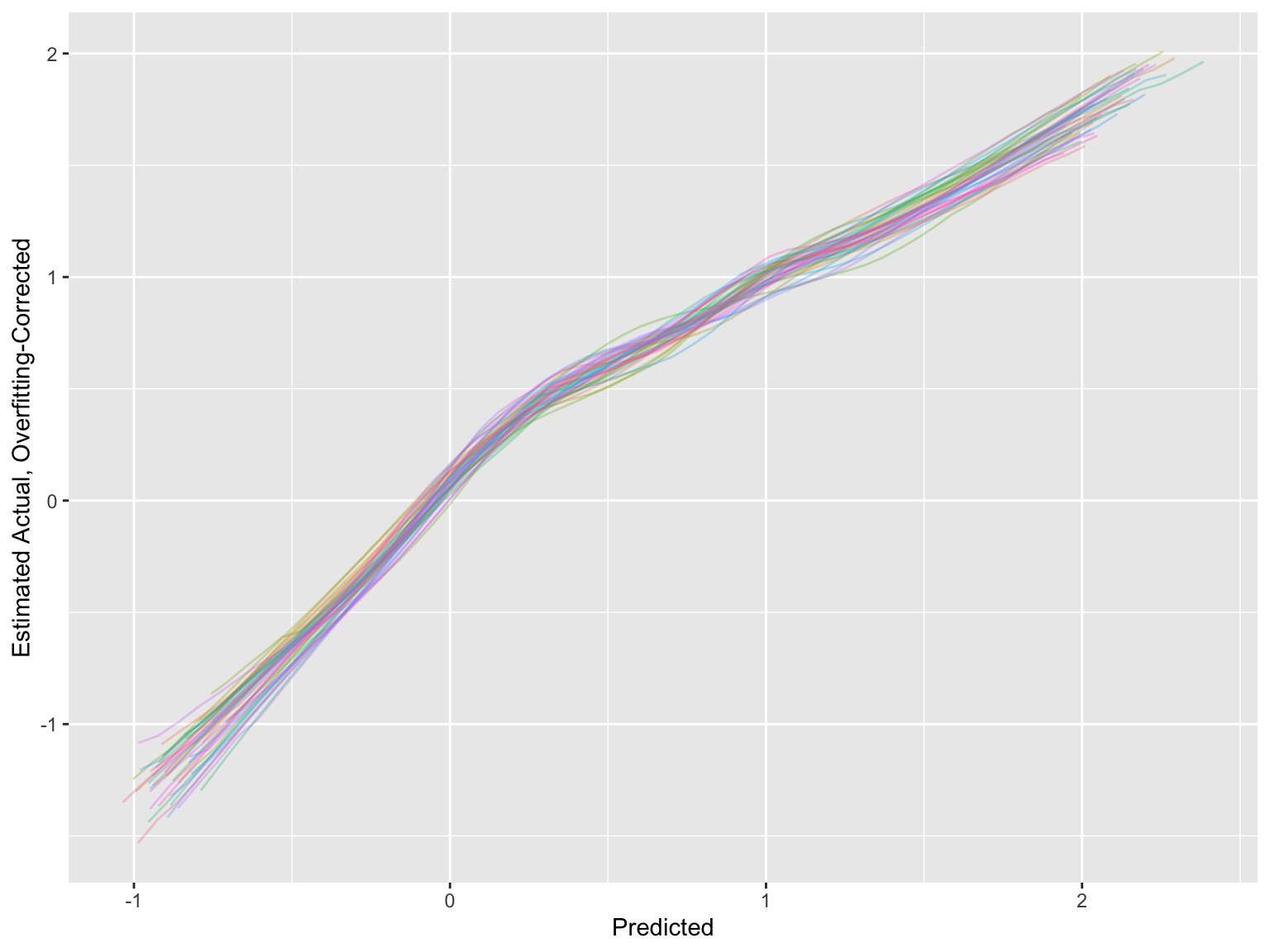
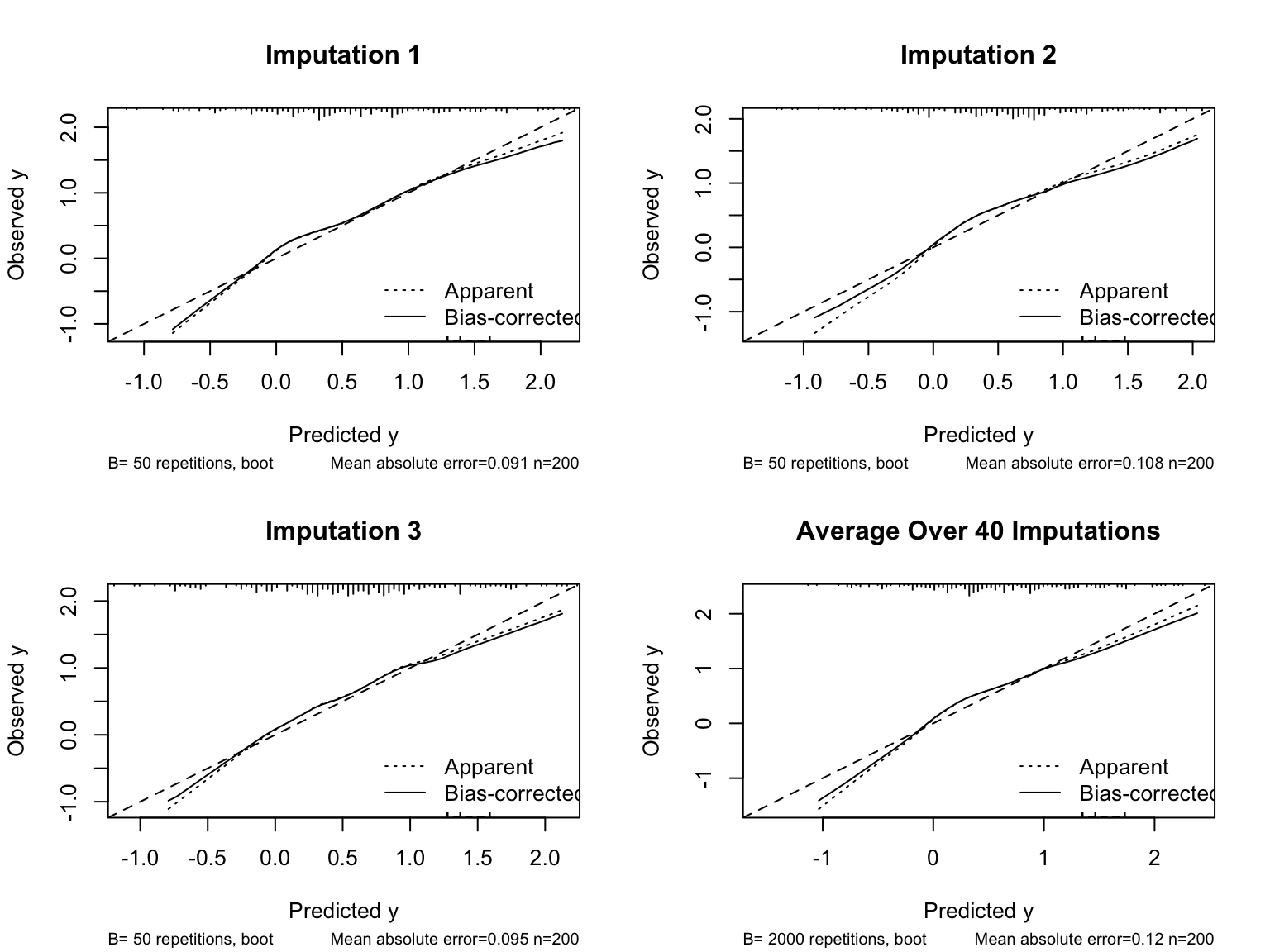
* For the estimated calibration curves, `processMI` by default shows all the individual curves from all multiple imputations (set `plotall=FALSE` to suppress this)
* Use an option to also show the first three individual validations followed by the average
```{r}
#| fig.height: 6
#| fig.width: 8
#| column: screen-right
cal <- processMI(f, 'calibrate', nind=3)
```
* Run `plot(cal)` if you want to see a full size final average calibration
For related information see @mi25com and @awo25com and [de Mul et al 2026](https://www.jclinepi.com/article/S0895-4356(26)00034-X/fulltext).
<!-- NEW -->
### Validation of Data Reduction {#sec-val-dr}
A frequently asked question is whether or not unsupervised learning (data reduction) needs to be repeated inside an internal validation loop. See [this](https://stats.stackexchange.com/questions/239898) for some excellent discussion. Here are are few thoughts.
* To be safe, include fresh data reduction inside each loop
* If you want to take a slight risk you can do the data reduction once on the whole dataset, because of the following
* Principal components (especially minor components), variable and observation clustering, and redundancy analysis can be very unstable
* They way in which they are unstable is uninformed by $Y$, so this instability can work either for or against you
* Typically we are allowed to use procedures that don't always work in our favor
* Contrast this with stepwise variable selection, which always attempts to work in our favor by maximizing $R^2$
### Validation of Bayesian Models {#sec-val-bayes}
Ideas about model validation can be much different in a Bayesian modeling context. If a prior distribution on a regression coefficient is somewhat flat, that implies that very large values of the parameter are likely. So overfitting cannot officially occur in that setting. Valuable discussions about Bayesian validation issues can be found [here](https://t.co/KfZVwGfbJb) and [here](https://t.co/BmUhOLNvEu).
On the other hand, overfitting can damage out-of-sample predictive accuracy, and there are Bayesian Markov chain Monte Carlo shortcuts that provide leave-out-one cross-validation statistics on the gold standard log-likelihood metric. This is elegantly covered in [this Richard McElreath video](https://youtu.be/odGAAJDlgp8?si=F6gpXe1-h2BybBs1).
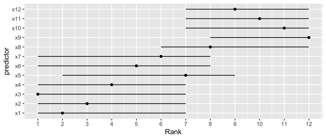
## Bootstrapping Ranks of Predictors {#sec-val-bootrank}
`r mrg(sound("v-12"))`
* Order of importance of predictors not pre-specified `r ipacue()`
* Researcher interested in determining "winners" and "losers"
* Bootstrap useful in documenting the difficulty of this task
* Get confidence limits of the rank of each predictor in the scale
of partial $\chi^2$ - d.f.
* Example using OLS
```{r cap='Bootstrap percentile 0.95 confidence limits for ranks of predictors in an OLS model. Ranking is on the basis of partial $\\chi^2$ minus d.f. Point estimates are original ranks',scap='Bootstrap confidence limits for ranks of predictors'}
#| label: fig-val-bootrank
#| fig-height: 3
# Use the plot method for anova, with pl=FALSE to suppress actual
# plotting of chi-square - d.f. for each bootstrap repetition.
# Rank the negative of the adjusted chi-squares so that a rank of
# 1 is assigned to the highest.  It is important to tell
# plot.anova.rms not to sort the results, or every bootstrap
# replication would have ranks of 1,2,3,... for the stats.
require(rms)
n <- 300
set.seed(1)
d <- data.frame(x1=runif(n), x2=runif(n), x3=runif(n), x4=runif(n),
                x5=runif(n), x6=runif(n), x7=runif(n), x8=runif(n),
             x9=runif(n), x10=runif(n), x11=runif(n), x12=runif(n))
d$y <- with(d, 1*x1 + 2*x2 +  3*x3  +  4*x4  + 5*x5 + 6*x6 + 7*x7 +
               8*x8 + 9*x9 + 10*x10 + 11*x11 + 12*x12 + 9*rnorm(n))

f <- ols(y ~ x1+x2+x3+x4+x5+x6+x7+x8+x9+x10+x11+x12, data=d)
B <- 1000
ranks <- matrix(NA, nrow=B, ncol=12)
rankvars <- function(fit)
  rank(plot(anova(fit), sort='none', pl=FALSE))
Rank <- rankvars(f)
for(i in 1:B) {    # 6s
  j <- sample(1:n, n, TRUE)
  bootfit <- update(f, data=d, subset=j)
  ranks[i,] <- rankvars(bootfit)
  }
lim <- t(apply(ranks, 2, quantile, probs=c(.025,.975)))
predictor <- factor(names(Rank), names(Rank))
w <- data.frame(predictor, Rank, lower=lim[,1], upper=lim[,2])
require(ggplot2)
ggplot(w, aes(x=predictor, y=Rank)) + geom_point() + coord_flip() +
  scale_y_continuous(breaks=1:12) +
  geom_errorbar(aes(ymin=lim[,1], ymax=lim[,2]), width=0)
```
<!-- NEW -->
See [this](https://fharrell.com/post/badb) and [this](https://hbiostat.org/talks/older/FHbiomarkers.pdf) for a higher-dimension example. See [this](https://www.tandfonline.com/doi/full/10.1080/10618600.2025.2547064?af=R#abstract) for a more in-depth discussion of ranking variable importance.
## Simplifying the Final Model by Approximating It {#sec-val-approx}
`r mrg(sound("v-13"))`
### Difficulties Using Full Models
* Predictions are conditional on all variables, standard errors `r ipacue()`
$\uparrow$ when predict for a low-frequency category
* Collinearity
* Can average predictions over categories to marginalize,
$\downarrow$ s.e.
### Approximating the Full Model
* Full model is gold standard `r ipacue()`
* Approximate it to any desired degree of accuracy
* If approx. with a tree, best c-v tree will have 1 obs./node
* Can use least squares to approx. model by predicting $\hat{Y} =
X\hat{\beta}$
* When original model also fit using least squares, coef. of
approx. model against $\hat{Y} \equiv$ coef. of subset of
variables fitted against $Y$ (as in stepwise)
* Model approximation still has some advantages `r ipacue()`
1. Uses unbiased estimate of $\sigma$ from full fit
1. Stopping rule less arbitrary
1. Inheritance of shrinkage
* If estimates from full model are $\hat{\beta}$ and approx.\
model is based on a subset $T$ of predictors $X$, coef. of approx.\
model are $W \hat{\beta}$, where <br> $W = (T'T)^{-1}T'X$
* Variance matrix of reduced coef.: $W V W'$
## How Do We Break Bad Habits? {#sec-val-habits}
`r mrg(sound("v-14"))`
* Insist on validation of predictive models and discoveries `r ipacue()`
* Show collaborators that split-sample validation is not
appropriate unless the number of subjects is huge
+ Split more than once and see volatile results
+ Calculate a confidence interval for the predictive accuracy in
the test dataset and show that it is very wide
* Run simulation study with no real associations and show that
associations are easy to find
* Analyze the collaborator's data after randomly permuting the $Y$
vector and show some positive findings
* Show that alternative explanations are easy to posit
+ Importance of a risk factor may disappear if 5 "unimportant"
risk factors are added back to the model
+ Omitted main effects can explain apparent interactions
+ _Uniqueness analysis_: attempt to predict the predicted
values from a model derived by data torture from all of the
features not used in the model
## Study Questions
**Section 5.1**
1. What is a general way to solve the problem of how to understand a
complex model?
1. Why is it useful to estimate the effect of changing a continuous
predictor on the outcome by varying the predictor from its $25^{th}$
to its $75^{th}$ percentile?
**Section 5.2**
1. Describe briefly in very general terms what the bootstrap involves.
1. The bootstrap may be used to estimate measures of many types of statistical quantities. Which type is being estimated when it comes to model validation?
**Section 5.3**
1. What are some disadvantages of external validation?
1. What would cause an independently validated $R^2$ to be negative?
1. A model to predict the probability that a patient has a disease was
developed using patients cared for at hospital A. Sort the
following in order from the worst way to validate the
predictive accuracy of a model to the best and most stringent way.
You can just specify the letters corresponding to the following, in
the right order.
a. compute the predictive accuracy of the model when applied to
a large number of patients in another country
a. compute the accuracy on a large number of patients in hospital
B that is in the same state as hospital A
a. compute the accuracy on 5 patients from hospital $A$ that were
collected after the original sample used in model fitting was completed
a. use the bootstrap
a. randomly split the data into two halves assuming that the
dataset is not extremely large; develop the model on
one half, freeze it, and evaluate the predictive accuracy on the other half
a. report how well the model predicted the disease status of
the patients used to fit the model
a. compute the accuracy on patients in hospital $A$ that were
admitted after the last patient's data used to fit the model were
collected, assuming that both samples were large
**Section 5.6**
1. What is a way to do a misleading interaction analysis?
1. What would cause the most embarrassment to a researcher who analyzed a high-dimensional dataset to find "winning" associations?
```{r echo=FALSE}
saveCap('05')
```
 Predictions plot from Rousseeuw (2026)