16  Transform-Both-Sides Regression

16.1 Background

• Challenges of traditional modeling (e.g. OLS) for estimation or inference
  • How should continuous predictors be transformed so as to get a good fit?
  • Is it better to transform the response variable? How does one find a good transformation that simplifies the right-hand side of the equation?
  • What if \(Y\) needs to be transformed non-monotonically (e.g., \(|Y - 100|\)) before it will have any correlation with \(X\)?
• Challenges from need for normality and equal variance assumptions to draw accurate inferences
  • If for the untransformed original scale of the response \(Y\) the distribution of the residuals is not normal with constant spread, ordinary methods will not yield correct inferences (e.g., confidence intervals will not have the desired coverage probability and the intervals will need to be asymmetric).
  • Quite often there is a transformation of \(Y\) that will yield well-behaving residuals. How do you find this transformation? Can you find a transformation for the \(X\)s at the same time?
  • All classical statistical inferential methods assume that the full model was pre-specified, that is, the model was not modified after examining the data. How does one correct confidence limits, for example, for data-based model and transformation selection?

16.2 Generalized Additive Models

• Hastie & Tibshirani (1990) developed GAMs for a variety of \(Y\) distributions
• Most GAMs are highly parametric, just relaxing assumptions about \(X\)
• Nonparametrically estimate all \(X\) transformations
• GAMs assume \(Y\) is already well transformed
• Excellent software for GAMs: R packages gam, mgcv, robustgam.

16.3 Nonparametric Estimation of \(Y\)-Transformation

There are a few approaches that also estimate the \(Y\)-transformation

16.3.1 ACE

• Breiman & Friedman (1985): alternating conditional expectation (ACE)
• Simultaneously transforms \(X\) and \(Y\) to maximize \(R^2\)

\[g(Y) = f_{1}(X_{1}) + f_{2}(X_{2}) + \ldots + f_{p}(X_{p}) \tag{16.1}\]

• Allows analyst to impose monotonicity restrictions on transformations
• Categorical \(X\) automatically numerically scored
• \(Y\)-transform allowed to be non-monotonic
  • can create an identifiability problem
• Estimates maximal correlation between \(X\) and \(Y\)
• Basis for nonparametric estimation for continuous \(X\): “super smoother” (R supsmu function)

16.3.2 AVAS

• Tibshirani (1988): additivity and variance stabilization (AVAS)
• Forces \(g(Y)\) to be monotonic
• Maximizes \(R^2\) while forcing \(g(Y)\) to have nearly constant variance of residuals
• Model specification still Equation 16.1

16.3.3 Overfitting

• Estimating so many transformations, especially \(g(Y)\) effectively adds many parameters to the model
• Results in overfitting (\(R^2\) inflation)
• Also no inferential measures provided
• Use the bootstrap to correct apparent \(R^2\) (\(R^{2}_{app}\)) for overfitting
• Estimates the optimism (bias) in \(R^{2}_{app}\) and subtracts this optimism from \(R^{2}_{app}\) to get an optimism-corrected estimate
• Also used to compute confidence limits for all estimated transformations
• And for predictor partial effects
• Must repeat all supervised learning steps afresh for each resample
• Limited testing has shown that the sample size needs to exceed 100 for ACE and AVAS to provide stable estimates

16.4 Obtaining Estimates on the Original Scale

• Traditional approach: take transformations of \(Y\) before fitting
• Logarithm is the most common transformation.¹
• If residuals on \(g(Y)\) have median 0, inverse transformed predicted values estimate median \(Y | X\) (quantiles are transformation-preserving, unlike mean)
• How to estimate general parameters such as means on original \(Y\) scale?
• Easy of residuals known to be Gaussian
• More general: Duan (1983) “smearing estimator”
• One-sample case, log transformation
  • \(\hat{\theta} = \sum_{i=1}^{n} \log(Y_{i})/n\),
  • residuals from this fitted value are given by \(e_{i} = \log(Y_{i}) - \hat{\theta}\)
  • smearing estimator of the population mean is \(\sum \exp(\hat{\theta} + e_{i})/n\)
  • is the ordinary sample mean \(\overline{Y}\)
• Smearing estimator needed when doing regression
• Regression run on \(g(Y)\)
  • estimated values \(\hat{g}(Y_{i}) = X_{i}\hat{\beta}\)
  • residuals on transformed scale \(e_{i} = \hat{g}(Y_{i}) - X_{i}\hat{\beta}\)
• Without restricting ourselves to estimating the population mean, let \(W(y_{1}, y_{2}, \ldots, y_{n})\) denote any function of a vector of untransformed response values
• To estimate the population mean in the homogeneous one-sample case, \(W\) is the simple average of all of its arguments
• To estimate the population 0.25 quantile, \(W\) is the sample 0.25 quantile of \(y_{1}, \ldots, y_{n}\)
• Smearing estimator of the population parameter estimated by \(W\) given \(X\) is \(W(g^{-1}(a + e_{1}), g^{-1}(a + e_{2}), \ldots, g^{-1}(a + e_{n}))\), where \(g^{-1}\) is the inverse of the \(g\) transformation and \(a = X\hat{\beta}\)
• With AVAS algorithm, monotonic transformation \(g\) is estimated from the data
• Predicted value of \(\hat{g}(Y)\) from Equation 16.1
• Extend the smearing estimator as \(W(\hat{g}^{-1}(a + e_{1}), \ldots, \hat{g}^{-1}(a + e_{n}))\), where \(a\) is the predicted transformed response given \(X\)
• \(\hat{g}\) is nonparametric (i.e., a table look-up)
• R areg.boot function computes \(\hat{g}^{-1}\) using reverse linear interpolation
• If assume residuals from \(\hat{g}(Y)\) assumed to be symmetrically distributed, their population median is zero
• Then can estimate the median on the untransformed scale by computing \(\hat{g}^{-1}(X\hat{\beta})\) ².
• For estimating quantiles of \(Y\), quantile regression (Koenker & Bassett, 1978) is more direct; see Austin et al. (2005) for a case study

¹ A disadvantage of transform-both-sides regression is this difficulty of interpreting estimates on the original scale. Sometimes the use of a special generalized linear model can allow for a good fit without transforming \(Y\).

² To be safe, areg.boot adds the median residual to \(X\hat{\beta}\) when estimating the population median (the median residual can be ignored by specifying statistic='fitted' to functions that operate on objects created by areg.boot)

16.5 R Functions

• R acepack package: ace and avas functions
• Hmisc areg.boot: R modeling language notation and also implements a parametric spline version; estimates partial effects on \(g(Y)\) and \(Y\) varying one of the \(X\)s over two values
• Resamples every part of modeling process, as with Faraway (1992)
• monotone function restricts a variable’s transformation to be monotonic
• I function restricts it to be linear

f <- areg.boot(Y ~ monotone(age) +
               sex + weight + I(blood.pressure))

plot(f)       #show transformations, CLs
Function(f)   #generate S functions
              #defining transformations
predict(f)    #get predictions, smearing estimates
summary(f)    #compute CLs on effects of each X
smearingEst() #generalized smearing estimators
Mean(f)       #derive S function to
              #compute smearing mean Y
Quantile(f)   #derive function to compute smearing quantile

The methods are best described in a case study.

16.6 Case Study

• Simulated data where conditional distribution of \(Y\) is log-normal given \(X\), but where transform-both-sides regression methods use un-logged \(Y\)
• Predictor \(X_1\) is linearly related to log \(Y\)
• \(X_2\) is related by \(|X_{2} - \frac{1}{2}|\)
• Categorical \(X_3\) has reference group \(a\) effect of zero, group \(b\) effect of 0.3, and group \(c\) effect of 0.5

require(rms)
set.seed(7)
n <- 400
x1 <- runif(n)
x2 <- runif(n)
x3 <- factor(sample(c('a','b','c'), n, TRUE))
y  <- exp(x1 + 2*abs(x2 - .5) + .3*(x3=='b') + .5*(x3=='c') +
          .5*rnorm(n))
# For reference fit appropriate OLS model
print(ols(log(y) ~ x1 + rcs(x2, 5) + x3), coefs=FALSE)

Linear Regression Model

ols(formula = log(y) ~ x1 + rcs(x2, 5) + x3)

	Model Likelihood Ratio Test	Discrimination Indexes
Obs 400	LR χ2 252.16	R2 0.468
σ 0.4826	d.f. 7	R2adj 0.458
d.f. 392	Pr(>χ2) 0.0000	g 0.510

Residuals

     Min       1Q   Median       3Q      Max 
-1.35353 -0.31381 -0.02378  0.32048  1.50329 

• Use 300 bootstrap resamples and run avas
• Only first 20 bootstraps are plotted
• Had we restricted x1 to be linear would have specified I(x1)

f  <- areg.boot(y ~ x1 + x2 + x3, method='avas', B=300)

f

avas Additive Regression Model

areg.boot(x = y ~ x1 + x2 + x3, B = 300, method = "avas")


Predictor Types

   type
x1    s
x2    s
x3    c

y type: s

n= 400   p= 3 

Apparent R2 on transformed Y scale: 0.46
Bootstrap validated R2            : 0.435

Coefficients of standardized transformations:

    Intercept            x1            x2            x3 
-1.020252e-15  1.065165e+00  1.165510e+00  1.000794e+00 


Residuals on transformed scale:

          Min            1Q        Median            3Q           Max 
-2.015488e+00 -5.182439e-01 -1.186501e-02  5.257140e-01  2.198222e+00 
         Mean          S.D. 
-2.997602e-17  7.328266e-01 

• Coefficients hard to interpret as scale of transformations arbitrary
• Model was very slightly overfitted (\(R^2\) dropped from 0.46 to 0.43), and \(R^2\) are in agreement with the OLS model fit
• Plot the transformations, 0.95 confidence bands, and a sample of the bootstrap estimates

spar(mfrow=c(2,2), ps=10)
plot(f, boot=20)

Figure 16.1: avas transformations: overall estimates, pointwise \(0.95\) confidence bands, and \(20\) bootstrap estimates (red lines).

• Nonparametrically estimated transformation of x1 almost linear
• Transformation of x2 is close to \(|x2 - 0.5|\)
• True transformation of y is \(\log(y)\), so variance stabilization and normality of residuals will be achieved if the estimated y-transformation is close to \(\log(y)\).

spar(bty='l')
ys <- seq(.8, 20, length=200)
ytrans <- Function(f)$y   # Function outputs all transforms
plot(log(ys), ytrans(ys), type='l')
abline(lm(ytrans(ys) ~ log(ys)), col=gray(.8))

Figure 16.2: Checking estimated against optimal transformation

• Approximate linearity = estimated transformation \(\log\)-like.³
• Obtain approximate tests of effects of each predictor
• summary sets all other predictors to reference values (e.g., medians)
• Compares predicted responses for a given level of the predictor \(X\) with predictions for lowest setting of \(X\)
• Default predicted response for summary is the median; tests are for differences in medians

³ Beware that use of a data–derived transformation in an ordinary model, as this will will result in standard errors that are too small. This is because model selection is not taken into account. (Faraway, 1992)

summary(f, values=list(x1=c(.2, .8), x2=c(.1, .5)))

summary.areg.boot(object = f, values = list(x1 = c(0.2, 0.8), 
    x2 = c(0.1, 0.5)))

Estimates based on 300 resamples



Values to which predictors are set when estimating
effects of other predictors:

      y      x1      x2      x3 
3.66995 0.50000 0.30000 2.00000 

Estimates of differences of effects on Median Y (from first X
value), and bootstrap standard errors of these differences.
Settings for X are shown as row headings.


Predictor: x1 
     
x     Differences       S.E Lower 0.95 Upper 0.95        Z     Pr(|Z|)
  0.2     0.00000        NA         NA         NA       NA          NA
  0.8     1.59603 0.5947651   0.430312   2.761748 2.683463 0.007286405


Predictor: x2 
     
x     Differences      S.E Lower 0.95 Upper 0.95         Z    Pr(|Z|)
  0.1    0.000000       NA         NA         NA        NA         NA
  0.5   -2.139942 1.164492  -4.422304  0.1424209 -1.837661 0.06611238


Predictor: x3 
   
x   Differences      S.E Lower 0.95 Upper 0.95         Z   Pr(|Z|)
  a   0.0000000       NA         NA         NA        NA        NA
  b   0.9653569 1.135403 -1.2599925   3.190706 0.8502327 0.3951957
  c   1.5631296 1.289487 -0.9642189   4.090478 1.2122102 0.2254319

• Example: when x1 increases from 0.2 to 0.8 predict an increase in median y by 1.55 with bootstrap standard error 0.21, when all other predictors are held to constants⁴
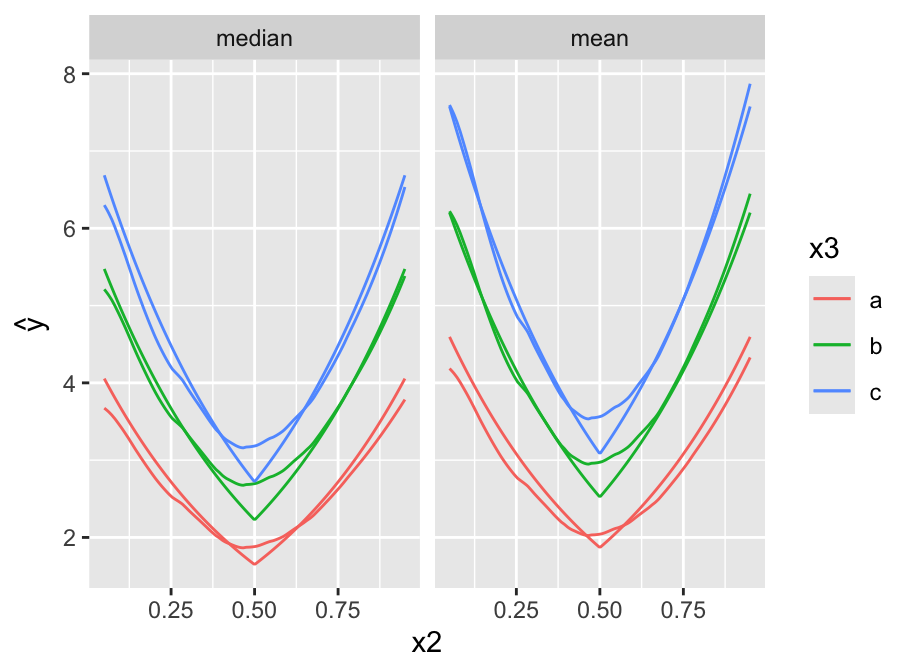
• Depict the fitted model by plotting predicted values
• x2 varies on \(x\)-axis, 3 curves correspond to three values of x3
• x1 set to 0.5
• Show estimates of both the median and the mean y.

⁴ Setting them to other constants will yield different estimates of the x1 effect, as the transformation of y is nonlinear.

require(ggplot2)
newdat <- expand.grid(x2=seq(.05, .95, length=200),
                      x3=c('a','b','c'), x1=.5,
                      statistic=c('median', 'mean'))
yhat <- c(predict(f, subset(newdat, statistic=='median'),
                  statistic='median'),
          predict(f, subset(newdat, statistic=='mean'),
                  statistic='mean'))
newdat <-
  upData(newdat,
         lp = x1 + 2*abs(x2 - .5) + .3*(x3=='b') +
              .5*(x3=='c'),
         ytrue = ifelse(statistic=='median', exp(lp),
           exp(lp + 0.5*(0.5^2))), print=FALSE)

ggplot(newdat, aes(x=x2, y=yhat, col=x3)) + geom_line() +
  geom_line(aes(x=x2, y=ytrue, col=x3)) +
  facet_wrap(~ statistic) + ylab(expression(hat(y)))

Figure 16.3: Predicted median (left panel) and mean (right panel) y as a function of x2 and x3. True population curves are pointed.

Austin, P. C., Tu, J. V., Daly, P. A., & Alter, D. A. (2005). Tutorial in Biostatistics:The use of quantile regression in health care research: A case study examining gender differences in the timeliness of thrombolytic therapy. Stat Med, 24, 791–816.

Breiman, L., & Friedman, J. H. (1985). Estimating optimal transformations for multiple regression and correlation (with discussion). J Am Stat Assoc, 80, 580–619.

Duan, N. (1983). Smearing estimate: A nonparametric retransformation method. J Am Stat Assoc, 78, 605–610.

Faraway, J. J. (1992). The cost of data analysis. J Comp Graph Stat, 1, 213–229.

Hastie, T., & Tibshirani, R. (1990). Generalized Additive Models. Chapman and Hall.

Koenker, R., & Bassett, G. (1978). Regression quantiles. Econometrica, 46, 33–50.

Tibshirani, R. (1988). Estimating transformations for regression via additivity and variance stabilization. J Am Stat Assoc, 83, 394–405.