```{r include=FALSE}
require(Hmisc)
options(qproject='rms', prType='html')
require(qreport)
getRs('qbookfun.r')
hookaddcap()
knitr::set_alias(w = 'fig.width', h = 'fig.height', cap = 'fig.cap', scap ='fig.scap')
```
<!-- NEW: base graphics -> ggplot2 -->
# Introduction to Survival Analysis
## Background
* Use when time to occurrence of event is important
* Don't just count events; event at 6m worse than event at 9y
* Response called _failure time, survival time, event time_
* Ex: time until CV death, light bulb failure, pregnancy,
ECG abnormality during exercise
* Allow for censoring
* Ex: 5y f/u study; subject still alive at 5y has failure time $5+$
* Length of f/u can vary
* Even in a well-designed randomized clinical trial, survival
modeling can allow one to
1. Test for and describe interactions with treatment. Subgroup analyses
can easily generate spurious results and they do not consider interacting
factors in a dose-response manner. Once interactions are modeled,
relative treatment benefits can be estimated (e.g., hazard ratios), and
analyses can be done to determine if some patients are too sick or too well to have even a relative benefit.
1. Understand prognostic factors (strength and shape).
1. Model absolute clinical benefit. First, a model for the probability
of surviving past time $t$ is developed. Then differences in
survival probabilities for patients on treatments A and B can be estimated.
The differences will be due primarily to sickness (overall risk)
of the patient and to treatment interactions.
1. Understand time course of treatment effect. The period of maximum
effect or period of any substantial effect can be estimated from
a plot of relative effects of treatment over time.
1. Gain power for testing treatment effects.
1. Adjust for imbalances in treatment allocation.
## Censoring, Delayed Entry, and Truncation
* Left-censoring
* Interval censoring
* Left-truncation (unknown subset of subjects who failed before
qualifying for the study)
* Delayed entry (exposure after varying periods of survival)
* Choice of time zero important
* Take into account _waiting time bias_
* Usually have random type I censoring (on duration, not # events)
* Must usually have _non-informative censoring_: <br>
censoring independent of impending failure
* Intention-to-treat is a preventative measure
## Notation, Survival, and Hazard Functions
* $T$: response variable
$$
S(t) = \Pr(T > t) = 1 - F(t)
$$
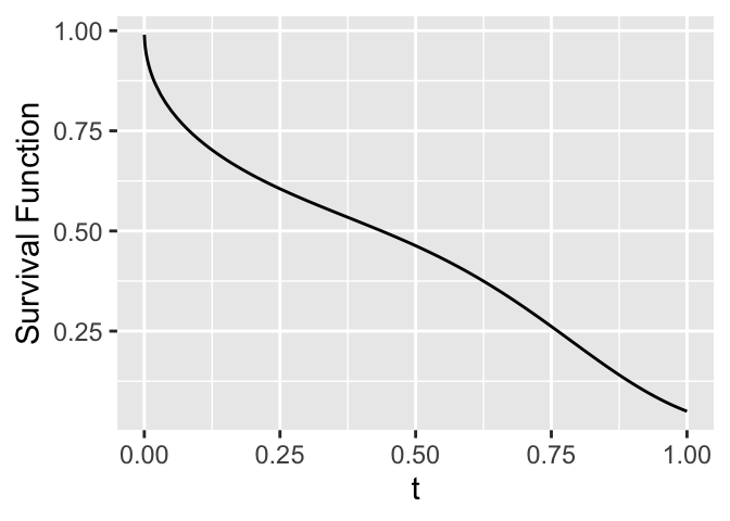
```{r fun-example,h=2.5,w=3.5,cap='Survival function'}
#| label: fig-surv-fun-example
tt <- c(seq(.0001,.002,by=.001),seq(.002,.02,by=.001),
        seq(.02,1,by=.01))
# Note: bb,dd not stated in usual Weibull form
aa <- .5
bb <- -.5
cc <- 10
dd <- 4
cumhaz <- (aa/(bb+1))*tt^(bb + 1) + (cc/(dd+1))*tt^(dd + 1)
survival <- exp(-cumhaz)
hazard <- ifelse(tt>.001, aa*tt^bb + cc*tt^dd, NA)
ggplot(mapping=aes(x=tt, y=survival)) + geom_line() +
  xlab(expression(t)) + ylab('Survival Function')
```
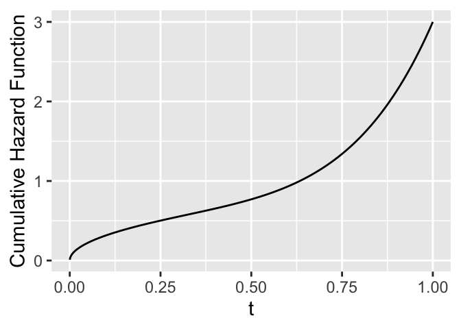
```{r cumhaz-example,h=2.5,w=3.5,cap='Cumulative hazard function'}
#| label: fig-surv-cumhaz-example
ggplot(mapping=aes(x=tt, y=cumhaz)) + geom_line() +
  xlab(expression(t)) + ylab('Cumulative Hazard Function')
```
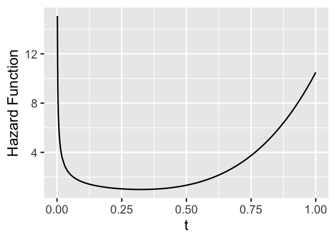
* Hazard function (force of mortality; instantaneous event rate)
* $\approx \Pr($event will occur in small interval around $t$ given
has not occurred before $t$)
* Very useful for learning about mechanisms and forces of risk
over time
```{r hazard-example,h=2.5,w=3.5,cap='Hazard function'}
#| label: fig-surv-hazard-example
ggplot(mapping=aes(x=tt, y=hazard)) + geom_line() +
  xlab(expression(t)) + ylab('Hazard Function')
```
$$
\lambda(t) = \lim_{u \rightarrow 0} \frac{\Pr(t < T \leq t+u | T>t)}{u},
$$
which using the law of conditional probability becomes
\begin{array}{ccc}
\lambda (t) &=& \lim_{u \rightarrow 0} \frac{\Pr(t < T \leq t+u) /
\Pr(T>t)}{u} \nonumber \\
&=& \lim_{u \rightarrow 0} \frac{[F(t+u)-F(t)]/u}{S(t)} \nonumber \\
&=& \frac{\partial F(t)/\partial t}{S(t)} \\
&=& \frac{f(t)}{S(t)} , \nonumber
\end{array}
$$
\frac{\partial \log S(t)}{\partial t} = \frac{\partial S(t)/\partial t}{S(t)} = -\frac{f(t)}{S(t)},
$$
$$
\lambda (t) = -\frac{\partial \log S(t)}{\partial t},
$$
$$
\int_{0}^{t}\lambda(v)dv = -\log S(t) .
$$
$$
\Lambda(t) = -\log S(t) ,
$$
$$
S(t) = \exp[-\Lambda(t)] .
$$
* Expected value of $\Lambda(T) = 1$
$$
T_{q} = S^{-1}(1-q) .
$$
$$
T_{0.5} = S^{-1}(0.5) .
$$
\begin{array}{ccc}
T_{q} &=& \Lambda^{-1}[-\log(1-q)] ~\text{and as a special case,} \nonumber \\
T_{.5} &=& \Lambda^{-1}(\log 2) .
\end{array}
$$
\mu = \int_{0}^{\infty}S(v)dv
$$
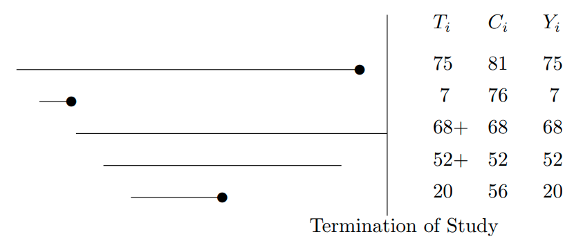
* Event time for subject $i$: $T_{i}$
* Censoring time: $C_{i}$
* Event indicator:
\begin{array}{ccc}
e_{i} &=& 1~~\text{if the event was observed}~~(T_{i} \leq C_{i}) , \nonumber \\
&=& 0~~\text{if the response was censored}~~(T_{i} > C_{i})
\end{array}
* The observed response is
$$
Y_{i} = \min(T_{i}, C_{i}) ,
$$
```{r out.width='85%',echo=FALSE}
#| label: fig-surv-censored-data
#| fig-cap: "Some censored data. Circles denote events."
knitr::include_graphics('images/surv-censored-data.png')
```
## Homogeneous Failure Time Distributions
* Exponential distribution: constant hazard
\begin{array}{ccc}
\Lambda(t) &=& \lambda t {\rm \ \ and} \nonumber \\
S(t) &=& \exp(-\Lambda(t)) = \exp(-\lambda t)
\end{array}
$$
T_{0.5} = \log(2)/\lambda
$$
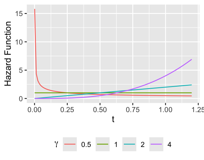
* Weibull distribution
\begin{array}{ccc}
\lambda(t) &=& \alpha \gamma t^{\gamma -1} \nonumber \\
\Lambda(t) &=& \alpha t^{\gamma} \\
S(t) &=& \exp(-\alpha t^{\gamma}) \nonumber
\end{array}
```{r weibull-shapes,h=2.75,w=3.5,cap='Some Weibull hazard functions with $\\alpha=1$ and various values of $\\gamma$'}
#| label: fig-surv-weibull-shapes
tt <- seq(1e-3, 1.2, length=100)
w <- NULL
a <- 1
for(b in c(.5, 1, 2, 4))
    w <- rbind(w, data.frame(gamma=b, tt=tt, y= a * b * tt ^ (b-1)))
ggplot(w, aes(x=tt, y=y, color=factor(gamma))) + geom_line() +
  xlab(expression(t)) + ylab('Hazard Function') +
    guides(color=guide_legend(title=expression(gamma))) +
  theme(legend.position='bottom')
```
$$
T_{0.5} =[(\log 2)/\alpha]^{1/\gamma}
$$
* The restricted cubic spline hazard model with $k$ knots is
$$
\lambda_{k}(t) = a + bt + \sum_{j=1}^{k-2} \gamma_{j} w_{j}(t)
$$
## Nonparametric Estimation of $S$ and $\Lambda$
### Kaplan--Meier Estimator
* No censoring $\rightarrow$
$$
S_{n}(t) =[{\rm number\ of\ } T_{i} > t]/n
$$
* Kaplan--Meier (product-limit) estimator
| Day | No. Subjects at Risk| Deaths | Censored | Cumulative Survival |
|-----|-----|-----|-----|-----|
| 12 | 100 | 1 | 0 | $99/100=.99$ |
| 30 | 99 | 2 | 1 | $97/99 \times 99/100 = .97$ |
| 60 | 96 | 0 | 3 | $96/96 \times .97 = .97$ |
| 72 | 93 | 3 | 0 | $90/93 \times .97 = .94$ |
| . | . | . | . | . |
| . | . | . | . | . |
$$
S_{{\rm KM}}(t) = \prod_{i:t_{i}<t}(1-d_{i}/n_{i})
$$
* The Kaplan--Meier estimator of $\Lambda(t)$ is $\Lambda_\text{KM}(t) = -\log S_{{\rm KM}}(t)$.
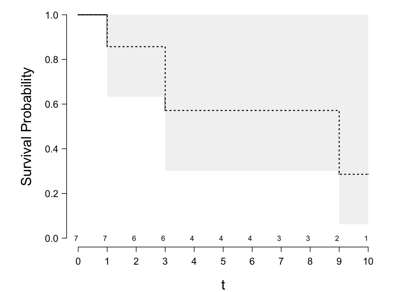
* Simple example
\begin{array}{c}
1 \ \ 3\ \ 3\ \ 6^{+}\ \ 8^{+}\ \ 9\ \ 10^{+} . \nonumber
\end{array}
| $i$ | $t_{i}$ | $n_{i}$ | $d_{i}$ | $(n_{i}-d_{i})/n_{i}$ |
|-----|-----|-----|-----|-----|
| 1 | 1 | 7 | 1 | 6/7 |
| 2 | 3 | 6 | 2 | 4/6 |
| 3 | 9 | 2 | 1 | 1/2 |
\begin{array}{ccc}
S_{\text{KM}}(t) &=& 1, ~~~~0 \le t<1 \nonumber \\
&=& 6/7=.85,~~1 \le t<3 \nonumber \\
&=& (6/7)(4/6)=.57,~~ 3 \le t<9 \\
&=& (6/7)(4/6)(1/2)=.29,~~9 \le t<10 . \nonumber
\end{array}
```{r km-example,scap='Kaplan-Meier and Nelson--Aalen estimates',cap='Kaplan--Meier product-limit estimator with 0.95 confidence bands. The Altschuler--Nelson--Aalen--Fleming--Harrington estimator is depicted with the dashed lines.'}
#| label: fig-surv-km-example
require(rms)
spar(bty='l')
tt <- c(1,3,3,6,8,9,10)
stat <- c(1,1,1,0,0,1,0)
S <- Surv(tt, stat)
# ggplot(npsurv(S ~ 1)) for prettier output if n.risk=FALSE
survplot(npsurv(S ~ 1), conf="bands", n.risk=TRUE, xlab="t")
survplot(npsurv(S ~ 1, type="fleming-harrington", conf.int=FALSE),
         add=TRUE, lty=3)
```
$$
\text{Var}(\log \Lambda_{{\rm KM}}(t)) = \frac{\sum_{i:t_{i} < t} d_{i} / [n_{i}(n_{i}-d_{i})]}
{\{\sum_{i:t_{i}<t} \log[(n_{i}-d_{i})/n_{i}]\}^{2}}
$$
$$
S_{\text{KM}}(t)^{\exp(\pm zs)}
$$
### Altschuler--Nelson Estimator
\begin{array}{ccc}
\hat{\Lambda}(t) &=& \sum_{i:t_{i}<t}\frac{d_{i}}{n_{i}} \nonumber \\
S_{\Lambda}(t) &=& \exp(-\hat{\Lambda}(t))
\end{array}
## Analysis of Multiple Endpoints
* Cancer trial: recurrence of disease or death
* CV trial: nonfatal MI or death
* Analyze usual way but watch out for differing risk factors
* Analyzing multiple causes of terminating event $\rightarrow$
+ Cause-specific hazards, censor on cause not currently analyzed
+ Not assume mechanism for cause removal or correlations of causes
+ Problem if apply to a setting where causes are removed differently
* More complex if explicitly handle mixture of nonfatal outcomes with fatal outcome
### Competing Risks
* Events independent $\rightarrow$ analyze separately, censoring others
* $\rightarrow$ unbiased estimate of cause-specific $\lambda(t)$ or $S(t)$
since censoring non-informative
* $1 - S_{\text{KM}}(t)$ estimates Pr(failing from the event in absence of other events)
* Method can work with dependent causes but interpretation difficult
* See @lar85mix for joint model of time until any failure and
the type of failure
* See @duc17smo for an interesting smooth
semi-nonparametric cumulative incidence estimator under competing
risks, incorporating a joint distribution of event time and type
### Competing Dependent Risks
* Ordinary K-M estimator biased
* Suppose cause $m$ is of interest
* Cause-specific hazard function:
$$\lambda_{m}(t) = \lim_{u \rightarrow 0} \frac{\Pr(\text{fail from cause}~m~ \text{in}~ [t, t+u) | \text{alive at} ~t)}{u}$$
* The _cumulative incidence function_ or probability of failure from cause $m$ by time $t$ is given by
$$
F_{m}(t) = \int_{0}^{t} \lambda_{m}(u)S(u)du
$$
where $S(u)$ is the probability of surviving (ignoring cause of death),
which equals
$\exp(-\int_{0}^{u}(\sum \lambda_{m}(x))dx)$
* Note that interpretation of cumulative incidence in the presence of competing risks can be difficult, e.g., probability of having a heart attack _that precedes death_
* $1-F_{m}(t) = \exp(-\int_{0}^{t}\lambda_{m}(u)du)$
only if failures due to other causes are eliminated and if the
cause-specific hazard of interest remains unchanged in doing so.
* Nonparametric estimator of $F_{m}(t)$:
$$
\hat{F}_{m}(t) = \sum_{i:t_{i}\leq t}\frac{d_{mi}}{n_{i}} S_{\text{KM}}(t_{i-1})
$$
where $d_{mi}$ is the number of failures of type $m$ at time $t_i$ and
$n_i$ is the number of subjects at risk of failure at $t_i$.
* @pep91inf, @pep91qua, @pep93kap show how to use combo of K-M estimators to estimate Pr(free of event 1 by time $t$ given event 2 not occur by $t$)
* Suppose event 1 not a terminating event (e.g., death); even after
event 1 subjects followed to find occurrences of event 2
* $\Pr(T_{1} > t | T_{2} > t)$:
\begin{array}{ccc}
\Pr(T_{1} > t | T_{2} > t) &=& \frac{\Pr(T_{1} > t ~\text{and} T_{2} > t)}{\Pr(T_{2} > t)} \nonumber \\
&=& \frac{S_{12}(t)}{S_{2}(t)},
\end{array}
where $S_{12}(t)$ is the survival function for $\min(T_{1},T_{2})$
* Estimate of Pr(subject still alive at $t$ will be free of MI at $t$): <br>$S_{\text{KM}_{12}} / S_{\text{KM}_{2}}$
* Can also easily compute Pr(event 1 occurs by time $t$ _and_
that event 2 has not occurred by $t$) $\rightarrow$ <br>
$S_{2}(t) - S_{12}(t) = [1 - S_{12}(t)] - [1 - S_{2}(t)]$
* _Crude survival functions_ come from _marginal distributions_,
i.e. $\Pr(T_{1} > t)$ whether or not event 2 occurs)
\begin{array}{ccc}
S_{c}(t) &=& 1 - F_{1}(t) \nonumber \\
F_{1}(t) &=& \Pr(T_{1} \leq t)
\end{array}
* $F_{1}(t)$ is _crude incidence function_
* $T_{1} < t \rightarrow$ occurrence of event 1 is part of the prob.
being computed
* Event 2 terminating $\rightarrow$ some subjects can never suffer event 1 $\rightarrow$ <br>
crude survival fctn. for $T_{1}$ never drops to zero
* Crude survival fctn interpreted as surv. dist. of
$W$ where $W=T_{1}$ if $T_{1} < T_{2}$ and $W=\infty$ otherwise
### State Transitions and Multiple Types of Nonfatal Events
Multiple live states, one absorbing state (all-cause mortality)
* @str98ext extended Kaplan--Meier estimator
* Estimate $\pi_{ij}(t_{1}, t_{2})$ that subject in state
$i$ at time $t_1$ is in state $j$ $t_2$ time units later
* Define $S_{KM}^{i}(t | t_{1})$ = Kaplan--Meier estimate of
Pr(surviving $t$ additional years for cohort of subjects
beginning follow-up at time $t_{1}$ in state $i$)
* Then
$$
\pi_{ij}(t_{1},t_{2}) = \frac{n_{ij}(t_{1},t_{2})}{n_{i}(t_{1},t_{2})}
S_{KM}^{i}(t_{2} | t_{1})
$$
where $n_{i}(t_{1},t_{2})$ is the number of subjects in live state $i$
at time $t_{1}$ who are alive and uncensored $t_{2}$ time units later, and
$n_{ij}(t_{1},t_{2})$ is the number of such subjects in state $j$
$t_{2}$ time units beyond $t_{1}$.
### Joint Analysis of Time and Severity of an Event
* Can give more weight to an event that occurs earlier or is
more severe
* @ber91ana
* Ordinal scale for severity
* Severity measured at time of (single) event
* Ex: time until first headache / severity of headache
* "joint hazard function", ordinal category $j$
$$
\lambda_{j}(t) = \lambda(t) \pi_{j}(t),
$$
* Allows shift in dist. of response severity as $t \uparrow$
### Analysis of Multiple Events
* Ex: MI, ulcer, pregnancy, infection
* Analysis of time to first event may lose info
* Specialized multivariate failure time methods exist
* Simpler to model _marginal distributions_
* One record per event per subject
* Can have # previous events as covariable
* Correct variances for intra-subject correlation using
clustered sandwich estimator
* Method can handle multiple events of differing types
### Generalization
Longitudinal ordinal models based on a discrete time state transition Markov process provide a unified framework for most of the contexts discussed in this chapter. See the last chapter of these RMS course notes and also [this](https://www.fharrell.com/talk/cmstat).
## R Functions
* `event.chart` in `Hmisc` draws a variety of charts for
displaying raw survival time data, for both single and multiple
events per subject (see also `event.history, event.chart2`)
* A general modeling approach makes use of ordinal semiparametric regression models (@sec-ordsurv)
* Analyses in this chapter can be done as special cases of the Cox
model
* Particular functions for this chapter (no covariables) from Therneau:
* `Surv` function: Combines time to event variable and
event/censoring indicator into a single survival time matrix object
* Right censoring: `Surv(y, event)`; `event` is
event/censoring indicator, usually coded `TRUE/FALSE`, 0=censored
1=event or 1=censored 2=event. If the event status variable has
other coding, e.g., 3 means death, use `Surv(y, s==3)`.
* `survfit`: Kaplan--Meier and other nonparametric survival
curves using the `survival` package
* `npsurv`: `rms` package wrapper for `survfit`
```{r eval=FALSE}
units(y) <- "Month"  # Default is "Day" - used for axis labels, etc.
survfit(Surv(y, event) ~ svar1 + svar2 + ... , data, subset,
        na.action=na.delete,
        type=c("kaplan-meier", "fleming-harrington", "fh2"),
        error=c("greenwood", "tsiatis"), se.fit=TRUE,
        conf.int=.95,
        conf.type=c("log", "plain", "log-log"))
```
If there are no stratification variables (`svar1`, ...), omit them.
To print a table of estimates, use
```{r eval=FALSE}
f <- survfit(...)
print(f)    # print brief summary of f
summary(f, times, censored=FALSE)
```
For failure times stored in days, use
```{r eval=FALSE}
f <- survfit(Surv(futime, event) ~ sex)
summary(f, seq(30,180,by=30))
```
to print monthly estimates.
To plot the object returned by `survfit`, use
```{r eval=FALSE}
plot(f, conf.int=TRUE, mark.time=TRUE, mark=3, col=1, lty=1,
     lwd=1, cex=1, log=FALSE, xscale=1, yscale=1,
     xlab="", ylab="", xaxs="S", ...)
```
This invokes `plot.survfit`. More options: use `npsurv`, `ggplot.npsurv`, and
`survplot` in `rms`
for other options that include automatic curve labeling and showing
the number of subjects at risk at selected times.
See code for @fig-surv-km-example above.
Stratified estimates, with four treatments
distinguished by line type and curve labels, could be drawn by
```{r eval=FALSE}
require(rms)
units(y) <- "Year"
f <- npsurv(Surv(y, stat) ~ treatment)
survplot(f, ylab="Fraction Pain-Free")
ggplot(f, ylab='Fraction Pain-Free')
```
* `bootkm` function in `Hmisc` bootstraps
Kaplan--Meier survival estimates or Kaplan--Meier estimates of
quantiles of the survival time distribution. It is easy to use
`bootkm` to compute for example a nonparametric confidence interval
for the ratio of median survival times for two groups.
```{r echo=FALSE}
saveCap('17')
```