```{r include=FALSE}
require(Hmisc)
require(qreport)
options(qproject='rms', prType='html')
getRs('qbookfun.r')
hookaddcap()
knitr::set_alias(w = 'fig.width', h = 'fig.height', cap = 'fig.cap', scap ='fig.scap')
```
# Case Study in Data Reduction {#sec-impred}
Recall that the aim of data reduction is to reduce (without using the
outcome) the number of parameters needed in the outcome model.
The following case study illustrates these techniques:
1. redundancy analysis;
1. variable clustering;
1. data reduction using principal component analysis (PCA), sparse
PCA, and pre\-transformations;
1. restricted cubic spline fitting using ordinary least squares,
in the context of scaling; and
1. scaling/variable transformations using canonical variates
and nonparametric additive regression.
## Data
Consider the 506-patient \index{datasets!prostate}prostate cancer
dataset from @bya80cho. The data are listed
in [@data; Table 46] and are
available at <https://hbiostat.org/data>.
These data were from a randomized trial comparing four treatments for
stage 3 and 4 prostate cancer, with
almost equal numbers of patients on placebo and each of three doses of
estrogen. Four patients had missing values on all of the following
variables:
`wt, pf, hx, sbp, dbp, ekg, hg, bm`; two of these patients were
also missing `sz`. These patients are excluded from
consideration. The ultimate goal of an analysis of the dataset might
be to discover patterns in survival or to do an analysis of covariance
to assess the effect of treatment while adjusting for patient
heterogeneity. See Chapter @sec-coxcase for such analyses.
The data reductions developed here are
general and can be used for a variety of dependent variables.
The variable names, labels, and a summary of the data are printed below. Because of extreme skewness, `ap` is log-transformed for the purpose of making its spike histogram.
```{r results='asis'}
require(Hmisc)
getHdata(prostate)  # Download and make prostate accessible
# Convert an old date format to R format
prostate$sdate <- as.Date(prostate$sdate)
d <- describe(prostate[2:17],
       trans=list(ap=list('log', log, exp)))
sparkline::sparkline(0)   # load sparkline javascript dependencies
maketabs(print(d, 'both'), initblank=TRUE, wide=TRUE)
```
`stage` is defined by `ap` as well as X-ray results. Of the
patients in stage 3, 0.92 have `ap` $\leq$ 0.8. Of those in stage 4,
0.93 have `ap` > 0.8. Since `stage` can be predicted almost
certainly from `ap`, we do not consider `stage` in some of the
analyses.
## How Many Parameters Can Be Estimated?
There are 354 deaths among the 502 patients. If predicting survival
time were of major interest, we could develop a reliable
model if no more than about $354/15 = 24$ parameters
were _examined_ against $Y$ in unpenalized modeling. Suppose that
a full model with no
interactions is fitted and that linearity is not assumed for any
continuous predictors. Assuming `age` is almost linear, we could
fit a restricted cubic spline function with three knots. For the other
continuous variables, let us use five knots. For categorical predictors,
the maximum number of degrees of freedom needed would be one fewer than
the number of categories. For `pf` we could lump the last two
categories since the last category has only 2 patients. Likewise, we
could combine the last two levels of `ekg`.
@tbl-impred-maxdf lists candidate
predictors with the maximum number of parameters we consider for each.
| Predictor: | `rx` | `age` | `wt` | `pf` | `hx` | `sbp` | `dbp` | `ekg` | `hg` | `sz` | `sg` | `ap` | `bm` |
|-----|-----|-----|-----|-----|-----|-----|-----|-----|-----|-----|-----|-----|-----|
| Number of Parameters: | 3 | 2 | 4 | 2 | 1 | 4 | 4 | 5 | 4 | 4 | 4 | 4 | 1 |
: Degrees of freedom needed for predictors {#tbl-impred-maxdf}
## Redundancy Analysis
As described in Section @sec-multivar-redun, it is occasionally useful to
do a rigorous redundancy analysis on a set of potential predictors.
Let us run the algorithm discussed there, on the set of predictors we
are considering. We will use a low threshold (0.3) for $R^2$ for
demonstration purposes.
```{r}
# Allow only 1 d.f. for three of the predictors
prostate <-
  transform(prostate,
            ekg.norm = 1*(ekg %in% c("normal","benign")),
            rxn = as.numeric(rx),
            pfn = as.numeric(pf))
# Force pfn, rxn to be linear because of difficulty of placing
# knots with so many ties in the data
# Note: all incomplete cases are deleted (inefficient)
r <- redun(~ stage + I(rxn) + age + wt + I(pfn) + hx +
           sbp + dbp + ekg.norm + hg + sz + sg + ap + bm,
           r2=.3, type='adjusted', data=prostate)
r
r2describe(r$scores, nvmax=4) # show strongest predictors of each variable
```
By any reasonable criterion on $R^2$, none of the predictors is
redundant. `stage` can be predicted with an $R^{2} = 0.658$ from
the other 13 variables, but only with $R^{2} = 0.493$ after deletion
of 3 variables later declared to be "redundant."
## Variable Clustering
From @tbl-impred-maxdf, the total number of parameters is
42, so some data reduction should be
considered. We resist the temptation to take the "easy way out"
using stepwise variable selection so that we can achieve a more stable
modeling process ^[@sau92boo used the bootstrap to demonstrate the variability of a standard variable selection procedure for the prostate cancer dataset.] and obtain
unbiased standard errors. Before using a variable
clustering procedure, note that `ap` is extremely skewed. To
handle skewness, we use Spearman rank correlations for continuous
variables (later we transform each variable using
`transcan`, which will allow ordinary correlation coefficients to
be used). After classifying `ekg` as "normal/benign" versus
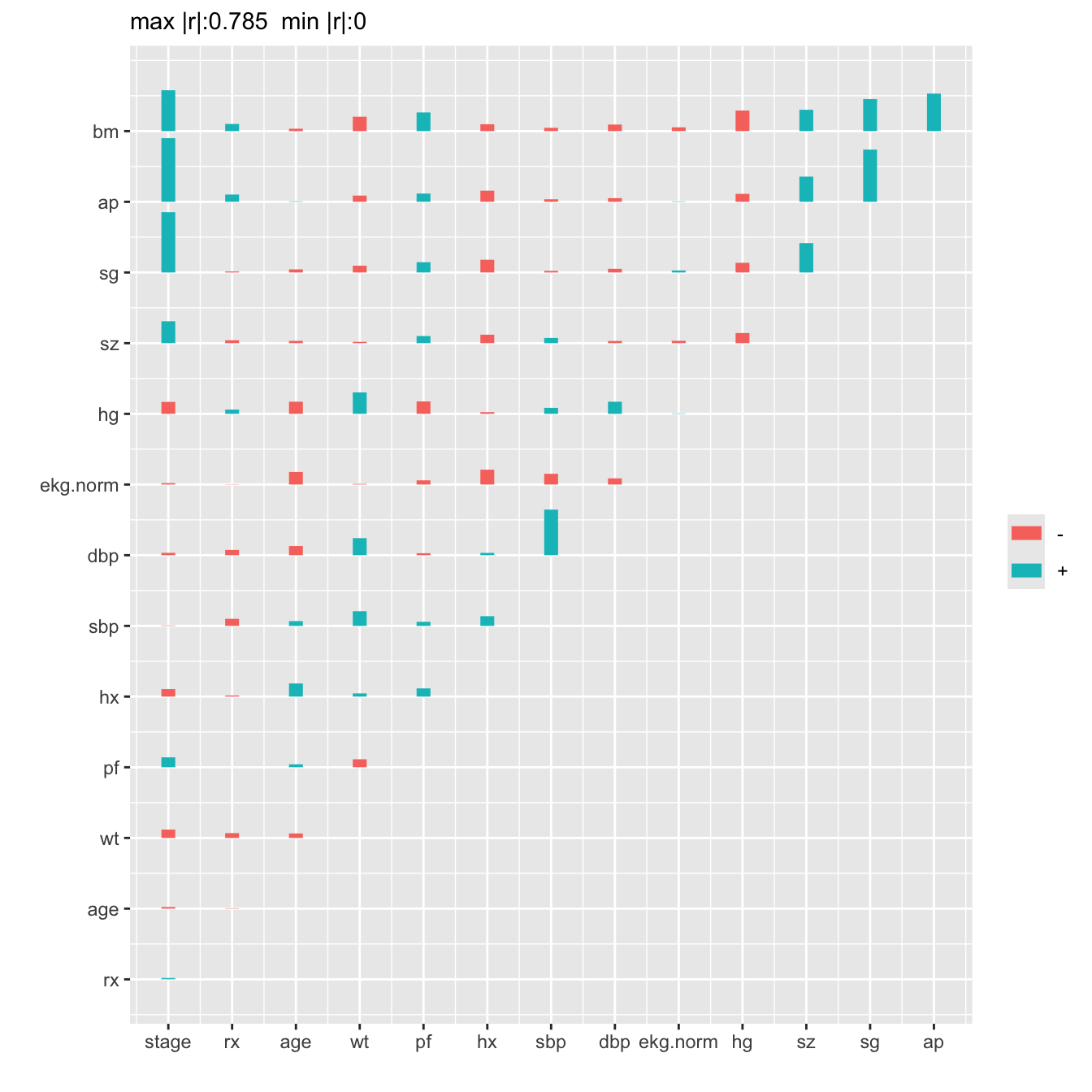
everything else, the Spearman correlations are plotted below.
```{r}
x <- with(prostate,
          cbind(stage, rx, age, wt, pf, hx, sbp, dbp,
                ekg.norm, hg, sz, sg, ap, bm))
# If no missing data, could use cor(apply(x, 2, rank))
r <- rcorr(x, type="spearman")$r    # rcorr in Hmisc
maxabsr <- max(abs(r[row(r) != col(r)]))
```
```{r spearman,h=7,w=7,cap='Matrix of Spearman $\\rho$ rank correlation coefficients between predictors. Horizontal gray scale lines correspond to $\\rho=0$. The tallest bar corresponds to $|\\rho|=0.785$.',scap='Spearman $\\rho$ rank correlations of predictors'}
#| label: fig-impred-spearman
plotCorrM(r)[[1]] # An Hmisc function
```
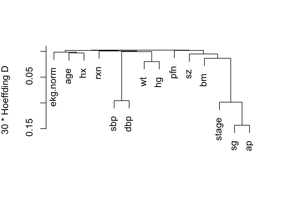
We perform a hierarchical
cluster analysis based on a similarity matrix that contains pairwise
Hoeffding $D$ statistics [@hoe48non] $D$ will detect
nonmonotonic associations.
```{r hclust,h=3.75,w=5,cap="Hierarchical clustering using Hoeffding's $D$ as a similarity measure. Dummy variables were used for the categorical variable `ekg. Some of the dummy variables cluster together since they are by definition negatively correlated.",scap="'Hierarchical clustering"}
#| label: fig-impred-hclust
vc <- varclus(~ stage + rxn + age + wt + pfn + hx +
              sbp + dbp + ekg.norm + hg + sz + sg + ap + bm,
              sim='hoeffding', data=prostate)
plot(vc)
```
We combine `sbp` and `dbp`, and tentatively combine
`ap, sg, sz`, and `bm`.
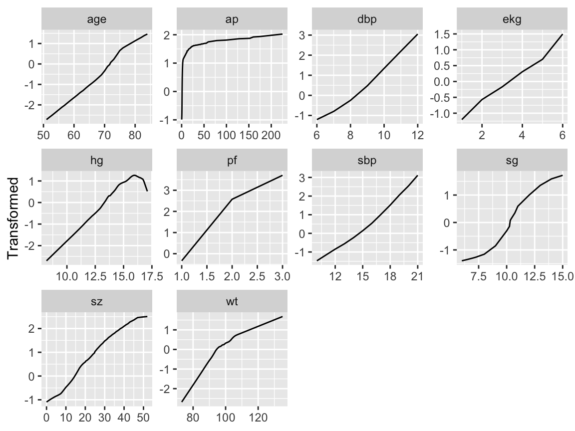
## Transformation and Single Imputation Using `transcan` {#sec-impred-transcan}
Now we turn to the scoring of the predictors to potentially reduce the
number of regression parameters that are needed later by doing away
with the need for nonlinear terms and multiple dummy variables.
The `R` `Hmisc` package `transcan` function
defaults to using a maximum generalized variance
method [@prinqual] that incorporates canonical variates to
optimally transform both sides of a multiple regression model. Each
predictor is treated in turn as a variable being predicted, and all
variables are expanded into restricted cubic splines (for continuous variables) or dummy variables (for categorical ones).
```{r transcan,w=6.5,h=5,cap='Simultaneous transformation and single imputation of all candidate predictors using `transcan`. Imputed values are shown as red plus signs. Transformed values are arbitrarily scaled to $[0,1]$.',scap='Simultaneous transformation and imputation using `transcan`'}
#| label: fig-impred-transcan
spar(bot=1)
# Combine 2 levels of ekg (one had freq. 1)
levels(prostate$ekg)[levels(prostate$ekg) %in%
                     c('old MI', 'recent MI')] <- 'MI'

prostate$pf.coded <- as.integer(prostate$pf)
# make a numeric version; combine last 2 levels of original
levels(prostate$pf) <- levels(prostate$pf)[c(1,2,3,3)]

ptrans <-
  transcan(~ sz + sg + ap + sbp + dbp +
           age + wt + hg + ekg + pf + bm + hx, imputed=TRUE,
           transformed=TRUE, trantab=TRUE, pl=FALSE,
           show.na=TRUE, data=prostate, frac=.1, pr=FALSE)
summary(ptrans, digits=4)
ggplot(ptrans, scale=TRUE) +
  theme(axis.text.x=element_text(size=6))
```
Note that at face value the transformation of `ap` was derived in a
circular manner,
since the combined index of stage and histologic grade, `sg`,
uses in its stage component a cutoff on `ap`. However, if `sg`
is omitted from consideration, the resulting transformation for `ap`
does not change appreciably. Note that `bm` and `hx` are
represented as binary variables, so their coefficients in the table of
canonical variable coefficients
are on a different scale. For the variables that were actually transformed,
the coefficients are for standardized transformed variables (mean 0,
variance 1). From examining the $R^2$s,
`age, wt, ekg, pf`, and `hx` are not
strongly related to other variables. Imputations for `age, wt, ekg`
are thus relying more on the median or modal values from the marginal
distributions.
From the coefficients of first (standardized) canonical variates,
`sbp` is predicted almost solely from `dbp`; `bm` is
predicted mainly from `ap, hg`, and `pf`. ^[@sch97pro used logistic models to impute dichotomizations of the predictors for this dataset.]
## Data Reduction Using Principal Components {#sec-impred-pc}
The first PC, PC$_{1}$, is the linear combination of standardized
variables having maximum variance. PC$_{2}$ is the linear
combination of predictors having the second largest variance such that
PC$_{2}$ is orthogonal to (uncorrelated with) PC$_{1}$. If there are
$p$ raw variables, the first $k$ PCs, where $k < p$, will explain only
part of the variation in the whole system of $p$ variables unless one
or more of the original variables is exactly a linear combination of
the remaining variables. Note that it is common to scale and center
variables to have mean zero and variance 1 before computing PCs.
The response variable (here, time until death due to any cause) is not
examined during data reduction, so that if PCs are selected by
variance explained in the $X$-space and not by variation explained in
$Y$, one needn't correct for model uncertainty or multiple comparisons.
PCA results in data reduction when the analyst uses only a subset of
the $p$ possible PCs in predicting $Y$. This is called
_incomplete principal component regression_.
When one sequentially enters PCs into a predictive model in a strict
pre-specified order (i.e., by descending amounts of variance explained
for the system of $p$ variables), model uncertainty requiring
bootstrap adjustment is minimized. In contrast, model uncertainty associated
with stepwise regression (driven by associations with $Y$) is massive.
For the prostate dataset, consider PCs
on raw candidate predictors, expanding polytomous factors using indicator variables.
The `R` function `princmp` is used, after singly imputing missing raw
values using `transcan`'s optimal additive nonlinear models. In
this series of analyses we ignore the treatment variable, `rx`. `princmp` calls the built-in `princomp` function. `princmp` assists with interpretation of PCs.
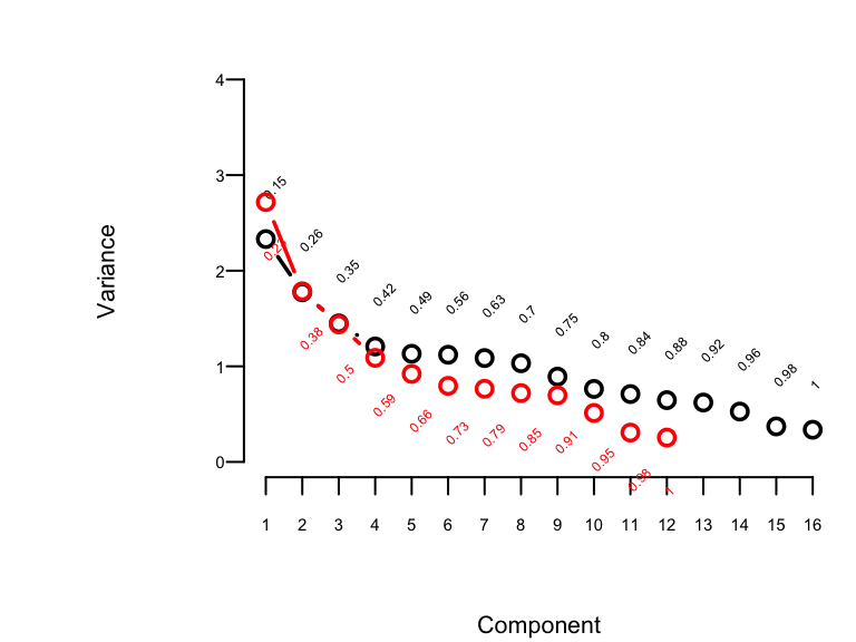
```{r pc,w=4,h=3,cap='Variance of the system of raw predictors (black) explained by individual principal components (lines) along with cumulative proportion of variance explained (text), and variance explained by components computed on `transcan`-transformed variables (red)',scap='Variance of the system explained by principal components.'}
#| label: fig-impred-pc
#| fig.width: 7
#| column: page-inset-right
spar(top=1, ps=7)
# Impute all missing values in all variables given to transcan
imputed <- impute(ptrans, data=prostate, list.out=TRUE)
imputed <- as.data.frame(imputed)

# Compute principal components on imputed data.  princmp will expand
# the categorical variable EKG into indicator variables.
# Use correlation matrix
pfn <- prostate$pfn
prin.raw <- princmp(~ sz + sg + ap + sbp + dbp + age +
          wt + hg + ekg + pfn + bm + hx,
          k=16, sw=TRUE, data=imputed)
prin.raw
plot(prin.raw, ylim=c(0,4), offset=1)
prin.trans <- princmp(ptrans$transformed, k=12)
prin.trans
plot(prin.trans, add=TRUE, col='red', offset=-1.3)
```
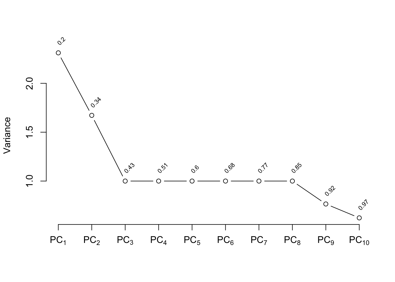
The plot shown in @fig-impred-pc is called a
"scree" plot [@jol10pri; pp. 96--99, 104, 106]. It shows the variation
explained by the first $k$ principal components as $k$ increases all
the way to 16 parameters (no data reduction). It requires 10
of the 16 possible components to explain $> 0.8$ of the variance,
and the first 5 components explain $0.49$ of the variance of the
system. Two of the 16 dimensions are almost totally redundant.
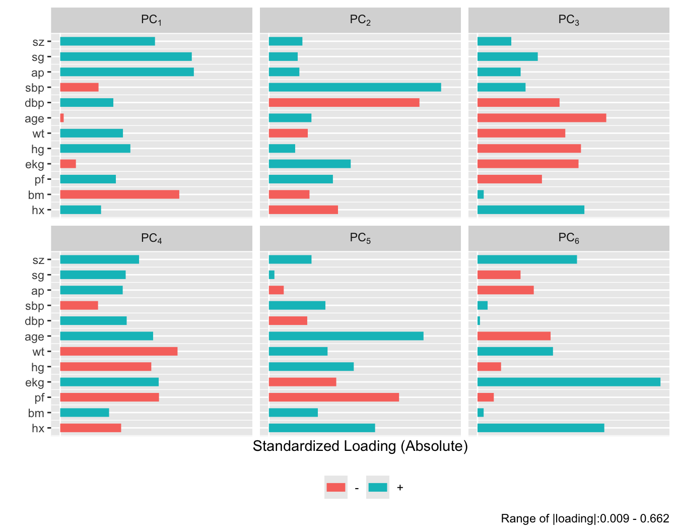
```{r}
#| fig-height: 7
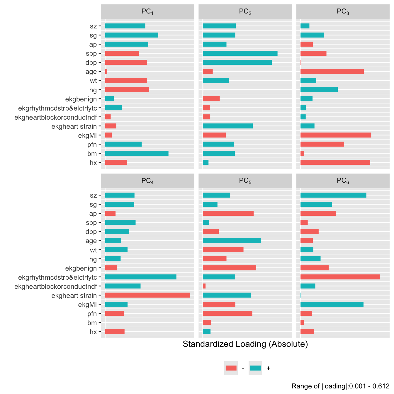
plot(prin.raw, 'loadings', k=6)
```
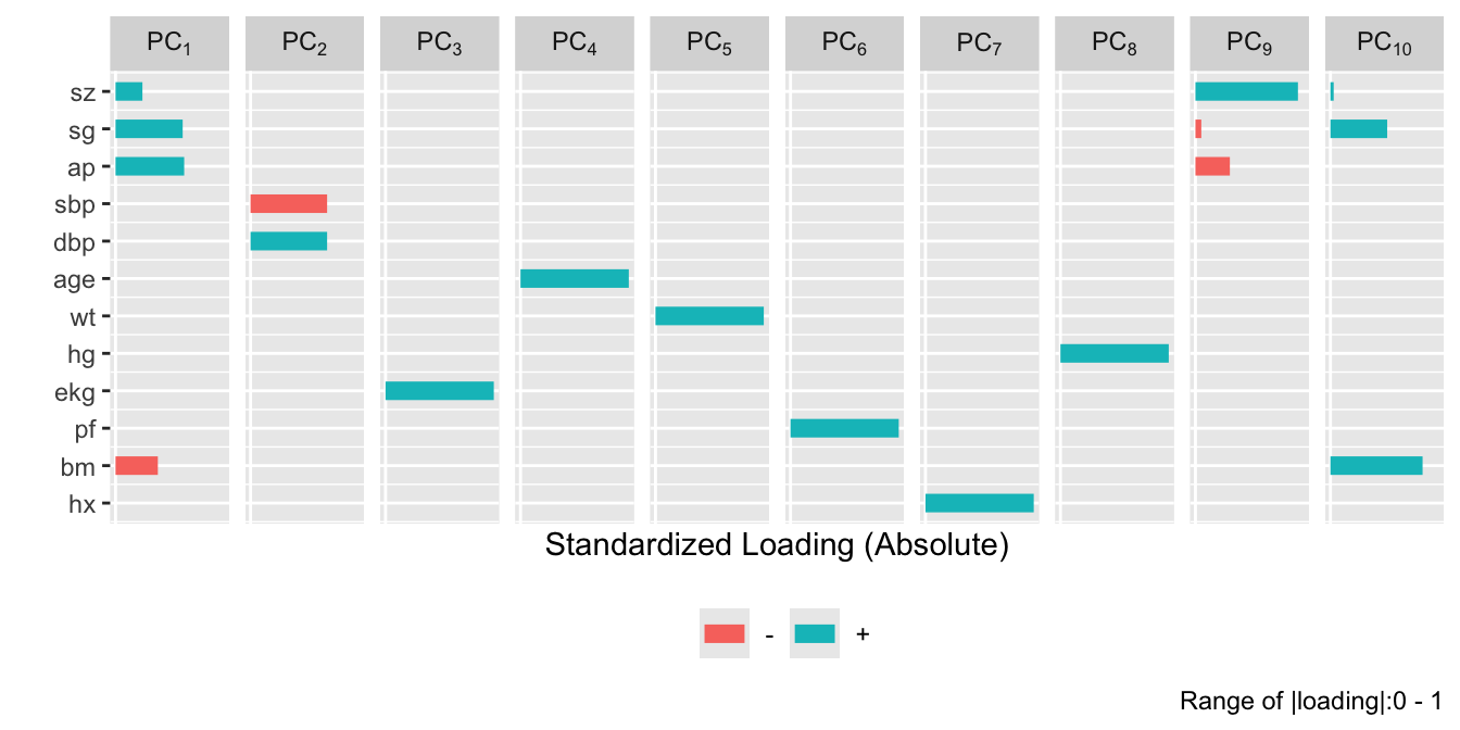
```{r}
#| fig-height: 5.5
plot(prin.trans, 'loadings', k=6)
```
After repeating this process when transforming all predictors via
`transcan`, we have only 12 degrees of freedom for the 12
predictors. The variance explained is depicted in @fig-impred-pc in red.
It requires at least 8 of the 12 possible components to explain $\geq 0.8$
of the variance, and the first 5 components explain $0.66$ of the
variance as opposed to $0.49$ for untransformed variables.
Let us see how the PCs "explain" the times until death using the
Cox regression [@cox72reg] function from `rms`, `cph`, described in
@sec-cox.
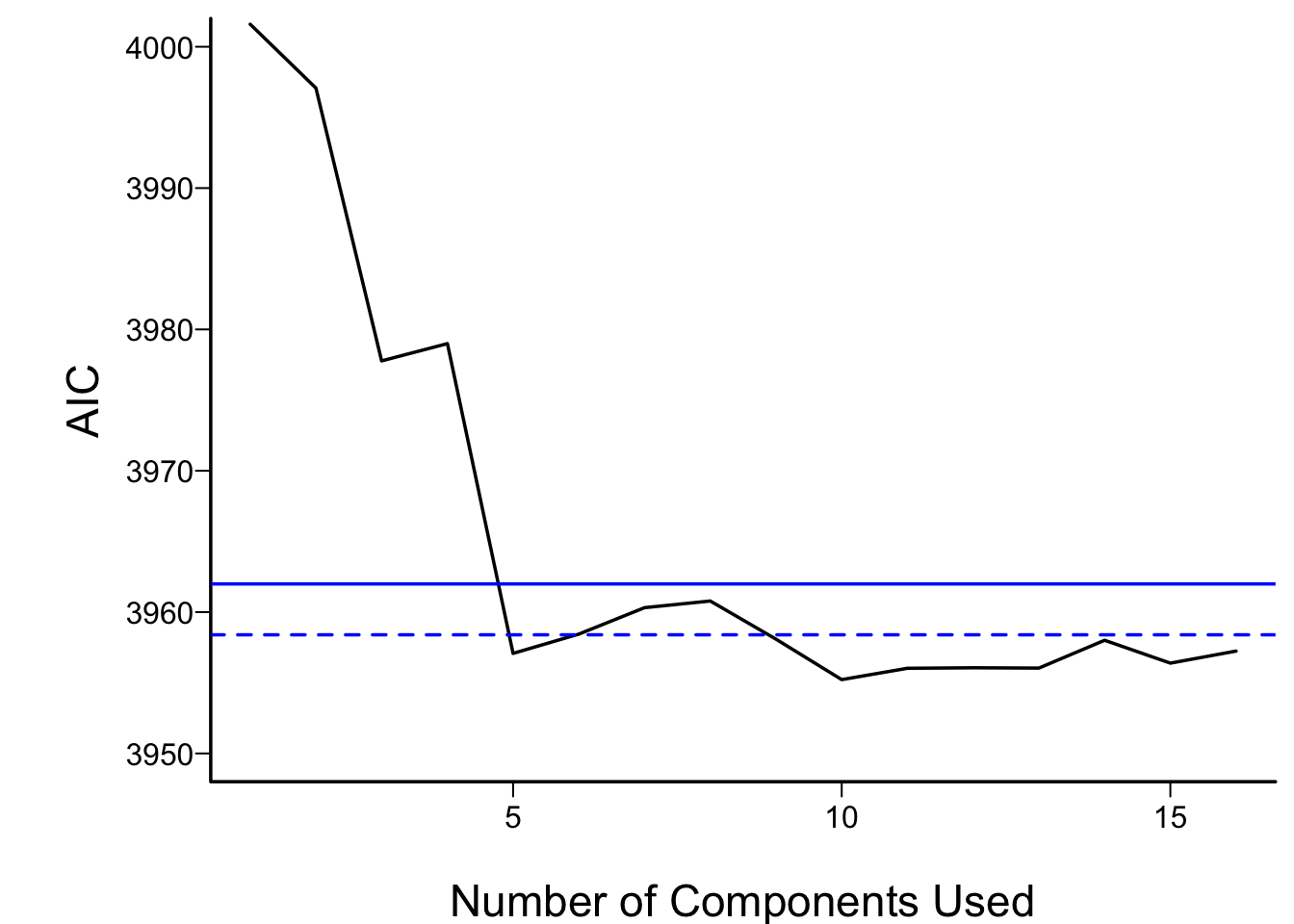
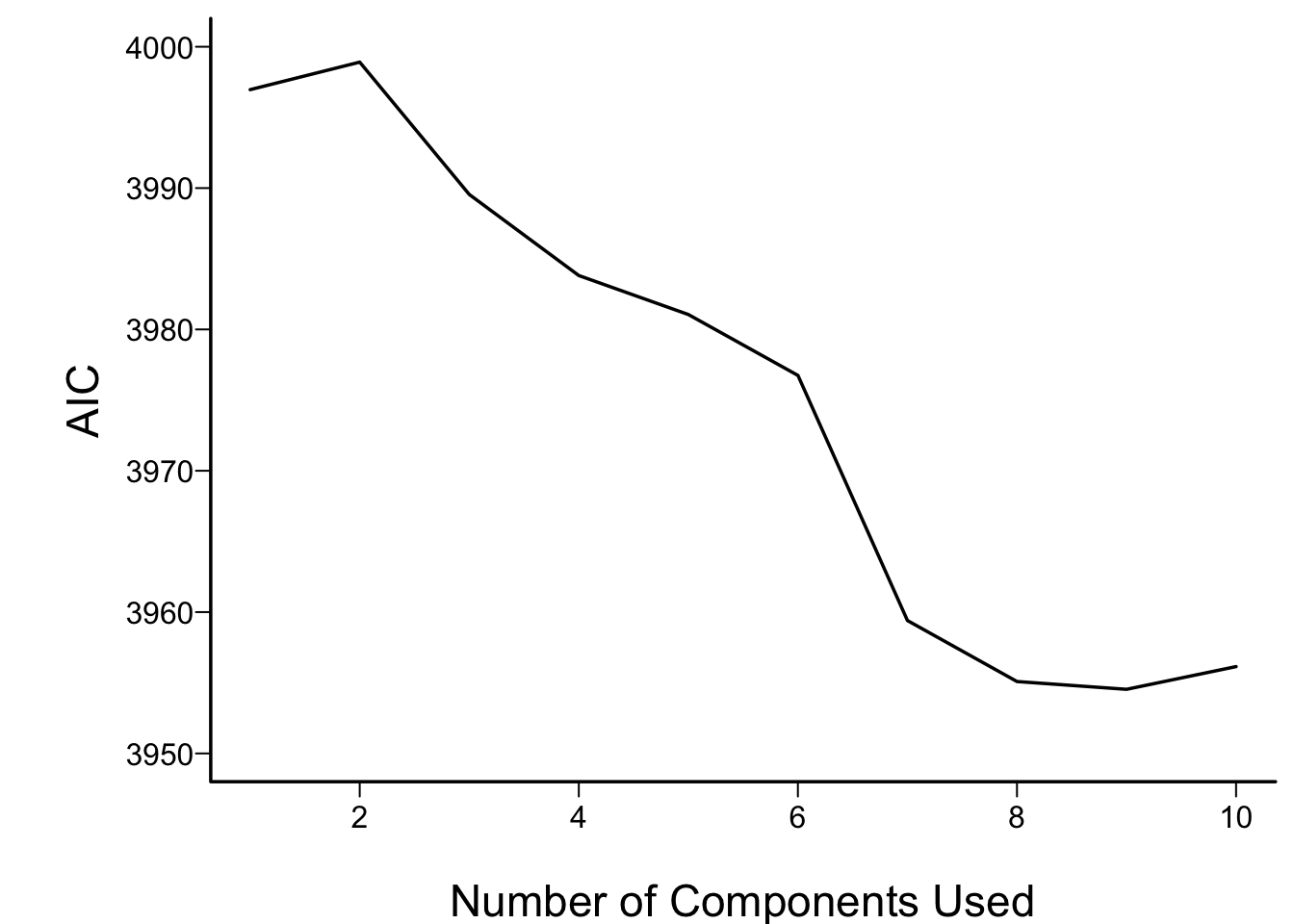
In what follows we vary the number of components used in
the Cox models from 1 to all 16, computing the AIC for each
model. AIC is related to model log likelihood penalized
for number of parameters estimated, and lower is better.
For reference, the AIC of the model using all of the original
predictors, and the AIC of a full additive spline model are shown as
horizontal lines.
```{r aic,cap='AIC of Cox models fitted with progressively more principal components. The solid blue line depicts the AIC of the model with all original covariates. The dotted blue line is positioned at the AIC of the full spline model.',scap='AIC vs. number of principal components'}
#| label: fig-impred-aic
require(rms)
spar(bty='l')
S <- with(prostate, Surv(dtime, status != "alive"))
# two-column response var.

pcs <- prin.raw$scores         # pick off all PCs
aic <- numeric(16)
for(i in 1:16) {
  ps <- pcs[,1:i]
  aic[i] <- AIC(cph(S ~ ps))
}
plot(1:16, aic, xlab='Number of Components Used',
     ylab='AIC', type='l', ylim=c(3950,4000))
f <- cph(S ~ sz + sg + log(ap) + sbp + dbp + age + wt + hg +
         ekg + pf + bm + hx, data=imputed)
abline(h=AIC(f), col='blue')
## The following model in the 2nd edition no longer converges
# f <- cph(S ~ rcs(sz,5) + rcs(sg,5) + rcs(log(ap),5) +
#          rcs(sbp,5) + rcs(dbp,5) + rcs(age,3) + rcs(wt,5) +
#          rcs(hg,5) + ekg + pf + bm + hx,
#          tol=1e-14, data=imputed)
f <- cph(S ~ rcs(sz,4) + rcs(sg,4) + rcs(log(ap),5) +
         rcs(sbp,4) + rcs(dbp,4) + rcs(age,3) + rcs(wt,4) +
         rcs(hg,4) + ekg + pf + bm + hx,
         tol=1e-14, data=imputed)
abline(h=AIC(f), col='blue', lty=2)
```
For the money, the first 5 components adequately summarizes all variables,
if linearly transformed, and the full linear model is no better than
this. The model allowing all continuous predictors to be nonlinear is
not worth its added degrees of freedom.
<!-- TODO The model allowing all continuous predictors to be nonlinear is--->
<!-- better than the linear full model but not b etter than the 5--->
<!-- component model.--->
Next check the performance of a model derived from cluster scores of
transformed variables.
```{r}
# Compute PC1 on a subset of transcan-transformed predictors
pco <- function(v) {
  f <- princmp(ptrans$transformed[,v])
    print(f)
  vars <- attr(f, 'results')$vars
  cat('Fraction of variance explained by PC1:',
      round(vars[1] / sum(vars),2), '\n')
  f$scores[,1]
}
tumor   <- pco(c('sz','sg','ap','bm'))
bp <- pco(c('sbp','dbp'))
cardiac <- pco(c('hx','ekg'))
# Get transformed individual variables that are not clustered
other   <- ptrans$transformed[,c('hg','age','pf','wt')]
f <- cph(S ~ tumor + bp + cardiac + other)  # other is matrix
AIC(f)
```
```{r}
print(f, long=FALSE, title='')
```
The `tumor` and `cardiac` clusters seem to dominate prediction
of mortality, and the AIC of the model built from cluster scores of
transformed variables compares favorably with other models
(@fig-impred-aic).
### Sparse Principal Components {#sec-impred-sparsepc}
A disadvantage of principal components is that every predictor
receives a nonzero weight for every component, so many coefficients
are involved even through the effective degrees of freedom with
respect to the response model are reduced. _Sparse principal components_ [@wit08tes] uses a penalty function to reduce the
magnitude of the loadings variables receive in the components. If an
L1 penalty is used (as with the
_lasso_, some loadings
are shrunk to zero, resulting in some simplicity. Sparse principal
components combines some elements of variable clustering, scoring of
variables within clusters, and
redundancy analysis.
@pcaPP have written a nice `R` package `pcaPP` for doing sparse PC
analysis.^[The `spcr` package is another sparse PC package that should also be considered.]
The following example uses the prostate data again.
To allow for nonlinear transformations and to score the `ekg`
variable in the prostate dataset down to a scalar, we use the
`transcan`-transformed predictors as inputs.
<!-- N% changed s$loadings to unclass() below--->
```{r spca,cap='Variance explained by individual sparse principal components (lines) along with cumulative proportion of variance explained (text)',scap='Sparse principal components'}
#| label: fig-impred-spca
s <- princmp(ptrans$transformed, k=10, method='sparse', sw=TRUE, nvmax=3)
s
plot(s)
```
```{r}
#| fig-height: 3.5
plot(s, 'loadings', nrow=1)
```
<!-- # Computing loadings on the original transcan scales--->
<!-- xtrans <- ptrans$transformed--->
<!-- cof <- matrix(NA, nrow=ncol(xtrans), ncol=10,--->
<!-- dimnames=list(colnames(xtrans), colnames(s$scores)))--->
<!-- for(i in 1:10) cof[,i] <- coef(lsfit(xtrans, s$scores[,i]))[-1]--->
<!-- tcof <- format(round(cof, 5))--->
<!-- tcof[abs(cof) < 1e-8] <- ''--->
<!-- print(tcof, quote=FALSE)--->
Only nonzero loadings are shown. The first sparse PC is the
`tumor` cluster used above, and the second is the blood pressure
cluster. Let us see how well incomplete sparse principal component
regression predicts time until death.
```{r spc,cap='Performance of sparse principal components in Cox models',scap='Performance of sparse principal components'}
#| label: fig-impred-spc
spar(bty='l')
pcs <- s$scores         # pick off sparse PCs
aic <- numeric(10)
for(i in 1:10) {
  ps <- pcs[,1:i]
  aic[i] <- AIC(cph(S ~ ps))
}
plot(1:10, aic, xlab='Number of Components Used',
     ylab='AIC', type='l',  ylim=c(3950,4000))
```
More components are required to optimize AIC than were seen in
@fig-impred-aic, but a model built from 6--8 sparse PCs
performed as well as the other models.
## Transformation Using Nonparametric Smoothers
The ACE nonparametric additive regression method of @bre85est transforms both the left-hand-side variable
and all the right-hand-side variables so as to optimize $R^{2}$. ACE
can be used to transform the predictors using
the `R` `ace` function in the `acepack`
package, called by the `transace` function in the
`Hmisc` package. `transace` does
not impute data but merely does casewise deletion of missing values.
Here `transace` is run after single imputation by `transcan`.
`binary` is used to tell `transace` which variables not to try
to predict (because they need no transformation). Several predictors
are restricted to be monotonically transformed.
```{r ace,h=4.5,w=6,cap='Simultaneous transformation of all variables using ACE.',scap='Transformation of variables using ACE'}
#| label: fig-impred-ace
f <- transace(~ monotone(sz) + monotone(sg) + monotone(ap) + monotone(sbp) +
                monotone(dbp) + monotone(age) + monotone(pf) + wt + hg +
                ekg + bm + hx, data=imputed)
f
ggplot(f)
```
Except for `ekg`, `age`, and for arbitrary sign reversals, the
transformations in @fig-impred-ace determined using
`transace` were similar to those in @fig-impred-transcan.
The `transcan` transformation for `ekg` makes more sense.
## Study Questions
**Section 8.2**
1. Critique the choice of the number of parameters devoted to each
predictor.
**Section 8.3**
1. Explain why the final amount of redundancy can change from the
initial assessment.
**Section 8.5**
1. What is the meaning of the first canonical variate?
1. Explain the first row of numbers in the matrix of coefficients of
canonical variates.
1. The transformations in Figure 8.3 are not optimal for predicting
the outcome. What good can be said of them?
**Section 8.6**
1. Why in general terms do principal components work well in
predictive modeling?
1. What is the advantage of sparse PCs over regular PCs?
```{r echo=FALSE}
saveCap('08')
```