```{r include=FALSE}
require(Hmisc)
options(qproject='rms', prType='html')
require(qreport)
getRs('qbookfun.r')
hookaddcap()
knitr::set_alias(w = 'fig.width', h = 'fig.height', cap = 'fig.cap', scap ='fig.scap')
```
# Binary Logistic Regression Case Study 1 {#sec-lrcase1}
**Case Study in Binary Logistic Regression, Model Selection and Approximation: Predicting Cause of Death**
## Overview
This chapter contains a case study on developing, describing, and
validating a binary logistic regression model. In addition, the
following methods are exemplified:
1. Data reduction using incomplete linear and nonlinear principal components
1. Use of AIC to choose from five modeling variations,
deciding which is best for the number of parameters
1. Model simplification using stepwise variable selection and
approximation of the full model
1. The relationship between the degree of approximation and the
degree of predictive discrimination loss
1. Bootstrap validation that includes penalization for model
uncertainty (variable selection) and that demonstrates a loss of
predictive discrimination over the full model even when compensating
for overfitting the full model.
The data reduction and pre-transformation methods used here were discussed in
more detail in @sec-impred. Single imputation will be
used because of the limited quantity of missing data.
## Background
Consider the randomized trial of estrogen for treatment of
prostate cancer [@bya80cho] described in @sec-impred. In
this trial, larger doses of estrogen reduced the effect of prostate
cancer but at the cost of increased risk of cardiovascular death.
@kay86tre did a formal analysis of the competing risks for
cancer, cardiovascular, and other deaths. It can also be quite
informative to study how treatment and baseline variables relate to
the cause of death for those patients who died. [@lar85mix] We
subset the original dataset of those patients dying from prostate
cancer ($n=130$), heart or vascular disease ($n=96$), or
cerebrovascular disease ($n=31$). Our goal is to predict
cardiovascular--cerebrovascular death (`cvd`, $n=127$) given the
patient died from
either `cvd` or prostate cancer. Of interest is whether the time
to death has an effect on the cause of death, and whether the
importance of certain variables depends on the time of death.
## Data Transformations and Single Imputation
In `R`, first obtain the desired subset of the data and do some preliminary
calculations such as combining an infrequent category with the next
category, and dichotomizing `ekg` for use in ordinary principal
components (PCs).
```{r}
require(rms)
options(prType='html')
getHdata(prostate)
prostate <-
  within(prostate, {
    levels(ekg)[levels(ekg) %in%
                c('old MI','recent MI')] <- 'MI'
    ekg.norm <- 1*(ekg %in% c('normal','benign'))
    levels(ekg) <- abbreviate(levels(ekg))
    pfn <- as.numeric(pf)
    levels(pf)  <- levels(pf)[c(1,2,3,3)]
    cvd <- status %in% c("dead - heart or vascular",
                         "dead - cerebrovascular")
    rxn = as.numeric(rx) })
# Use transcan to compute optimal pre-transformations
ptrans <-   # See Figure (* @fig-prostate-transcan*)
  transcan(~ sz + sg + ap + sbp + dbp +
           age + wt + hg + ekg + pf + bm + hx + dtime + rx,
           imputed=TRUE, transformed=TRUE,
           data=prostate, pl=FALSE, pr=FALSE)
# Use transcan single imputations
imp <- impute(ptrans, data=prostate, list.out=TRUE)
NAvars <- all.vars(~ sz + sg + age + wt + ekg)
for(x in NAvars) prostate[[x]] <- imp[[x]]
subset <- prostate$status %in% c("dead - heart or vascular",
    "dead - cerebrovascular","dead - prostatic ca")
trans <- ptrans$transformed[subset,]
psub  <- prostate[subset,]
```
## Regression on Original Variables, Principal Components and Pretransformations {#sec-lrcase1-pc}
We first examine the performance of data reduction in predicting the
cause of death, similar to what we did for survival time in
Section @sec-impred-pc. The
first analyses assess how well PCs (on raw and
transformed variables) predict the cause of death.
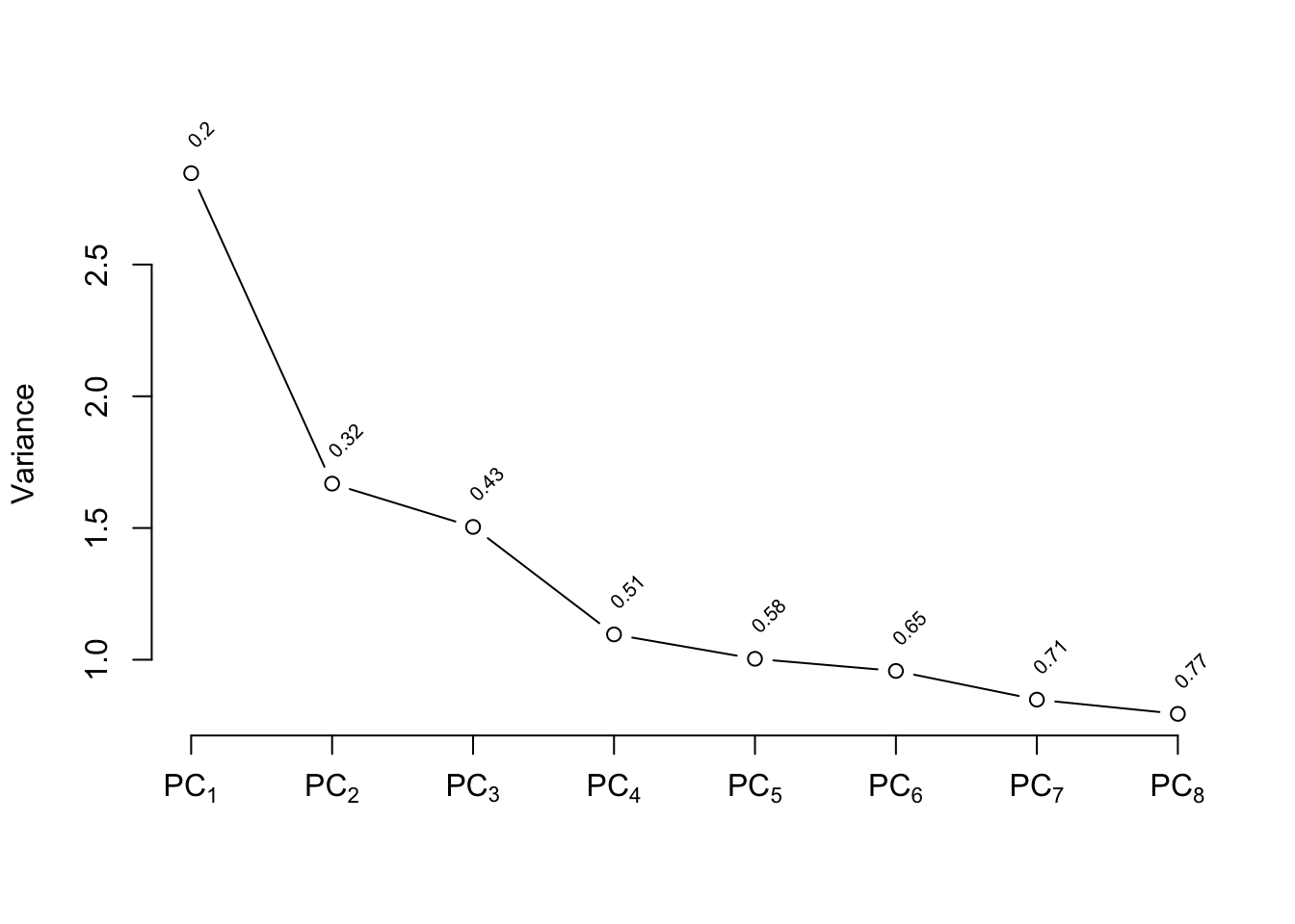
There are 127 `cvd`s. We use the 15:1 rule of thumb
discussed in @sec-multivar-overfit to justify using the
first 8 PCs. `ap` is log-transformed because of
its extreme distribution. We use `Hmisc::princmp`.
```{r}
# Compute the first 8 PCs on raw variables then on
# transformed ones
p <- princmp(~ sz + sg + log(ap) + sbp + dbp + age +
             wt + hg + ekg.norm + pfn + bm + hx + rxn + dtime,
             data=psub, k=8, sw=TRUE, kapprox=2)
p
plot(p)
```
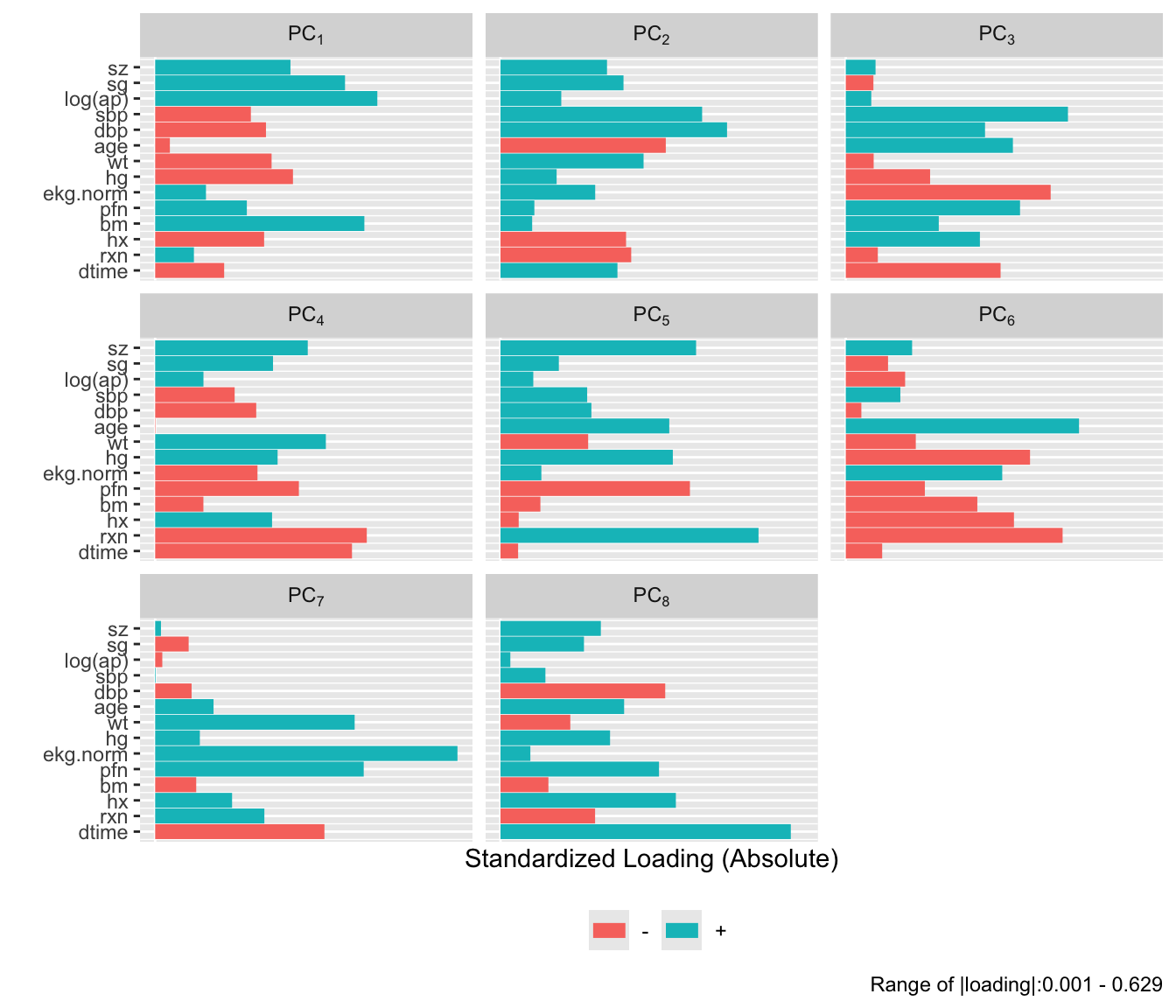
```{r}
#| fig-height: 6
plot(p, 'loadings')
```
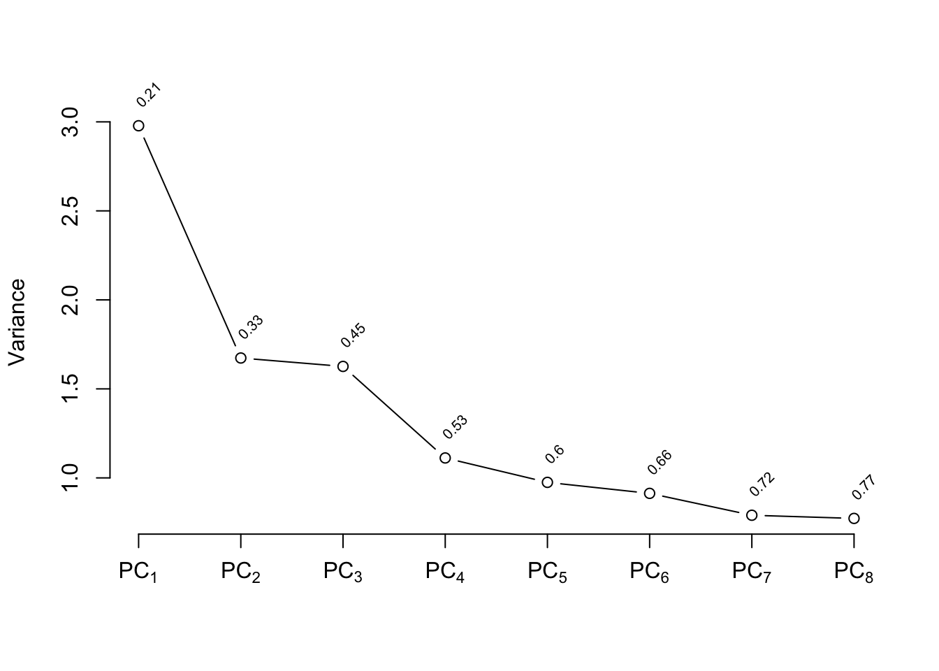
```{r}
pc8 <- p$scores
f8  <- lrm(cvd ~ pc8, data=psub)
p   <- princmp(trans, k=8, sw=TRUE, kapprox=2)
p
plot(p)
```
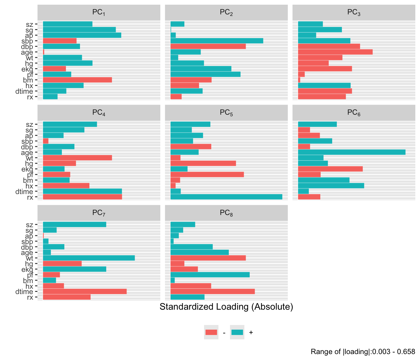
```{r}
#| fig-height: 6
plot(p, 'loadings')
```
```{r}
pc8t <- p$scores
f8t  <- lrm(cvd ~ pc8t, data=psub)
# Fit binary logistic model on original variables
# x=TRUE y=TRUE are for test='LR', validate, calibrate
f <- lrm(cvd ~ sz + sg + log(ap) + sbp + dbp + age +
         wt + hg + ekg + pf + bm + hx + rx + dtime,
                 x=TRUE, y=TRUE, data=psub)
# Expand continuous variables using splines
g <- lrm(cvd ~ rcs(sz,4) + rcs(sg,4) + rcs(log(ap),4) +
         rcs(sbp,4) + rcs(dbp,4) + rcs(age,4) + rcs(wt,4) +
         rcs(hg,4) + ekg + pf + bm + hx + rx + rcs(dtime,4),
         data=psub)
# Fit binary logistic model on individual transformed var.
h <- lrm(cvd ~ trans, data=psub)
```
The five approaches to modeling the outcome are compared using AIC
(where smaller is better).
```{r}
c(f8=AIC(f8), f8t=AIC(f8t), f=AIC(f), g=AIC(g), h=AIC(h))
```
Based on AIC, the more traditional model fitted to the raw data and assuming
linearity for all the continuous predictors has only a slight chance of
producing worse cross-validated predictive accuracy than other methods.
The chances are also good that effect estimates from this simple
model will have competitive mean squared errors.
## Description of Fitted Model
Here we describe the simple all-linear full model.
Summary statistics and Wald and likelihood ratio ANOVA tables are below, followed by partial effects plots with pointwise confidence bands, and odds ratios
over default ranges of predictors.
```{r}
f
anova(f)
an <- anova(f, test='LR')
an
```
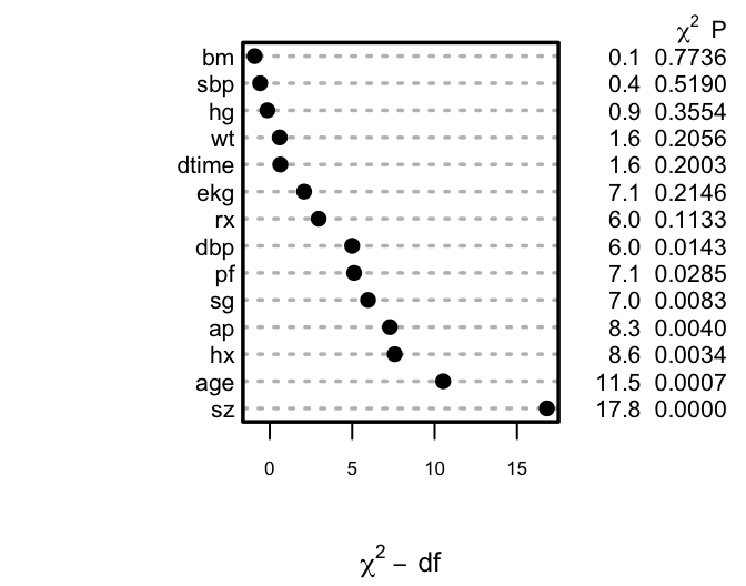
```{r h=2.75,w=3.5,cap='Ranking of apparent importance of predictors of cause of death using LR statistics'}
#| label: fig-lrcase1-full
spar(ps=8,top=0.5)
plot(an)
s <- f$stats
gamma.hat <- (s['Model L.R.'] - s['d.f.'])/s['Model L.R.']
```
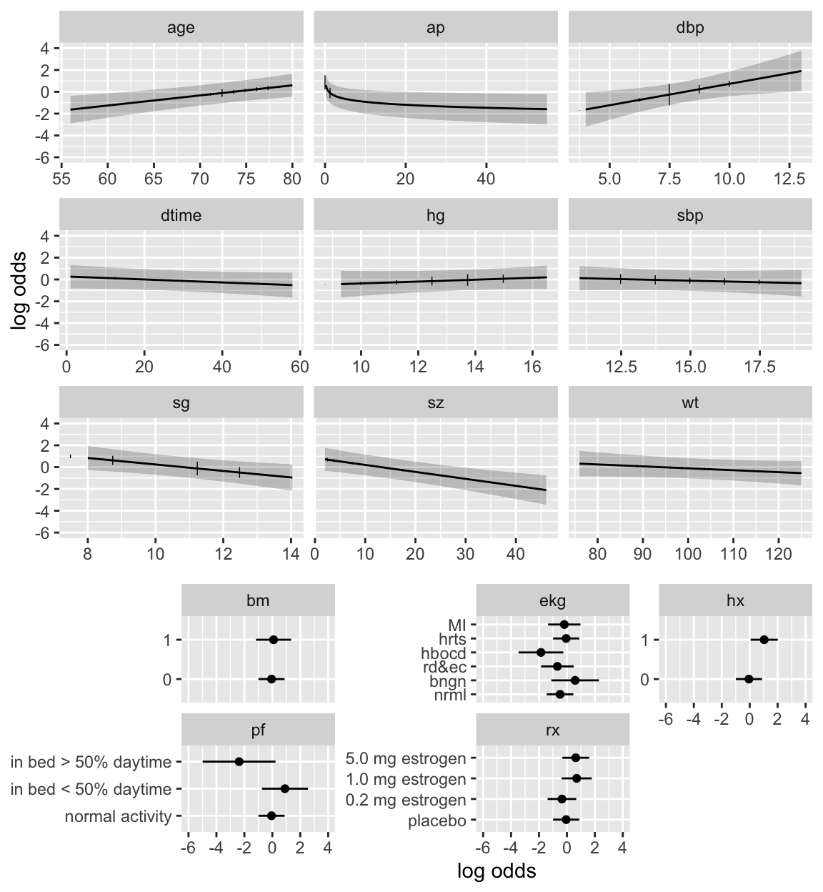
```{r h=6.5,w=6,cap='Partial effects (log odds scale) in full model for cause of death, along with vertical line segments showing the raw data distribution of predictors',scap='Partial effects in cause of death model'}
#| label: fig-lrcase1-fullpeffects
dd <- datadist(psub); options(datadist='dd')
ggplot(Predict(f), sepdiscrete='vertical', vnames='names',
       rdata=psub,
       histSpike.opts=list(frac=function(f) .1*f/max(f) ))
```
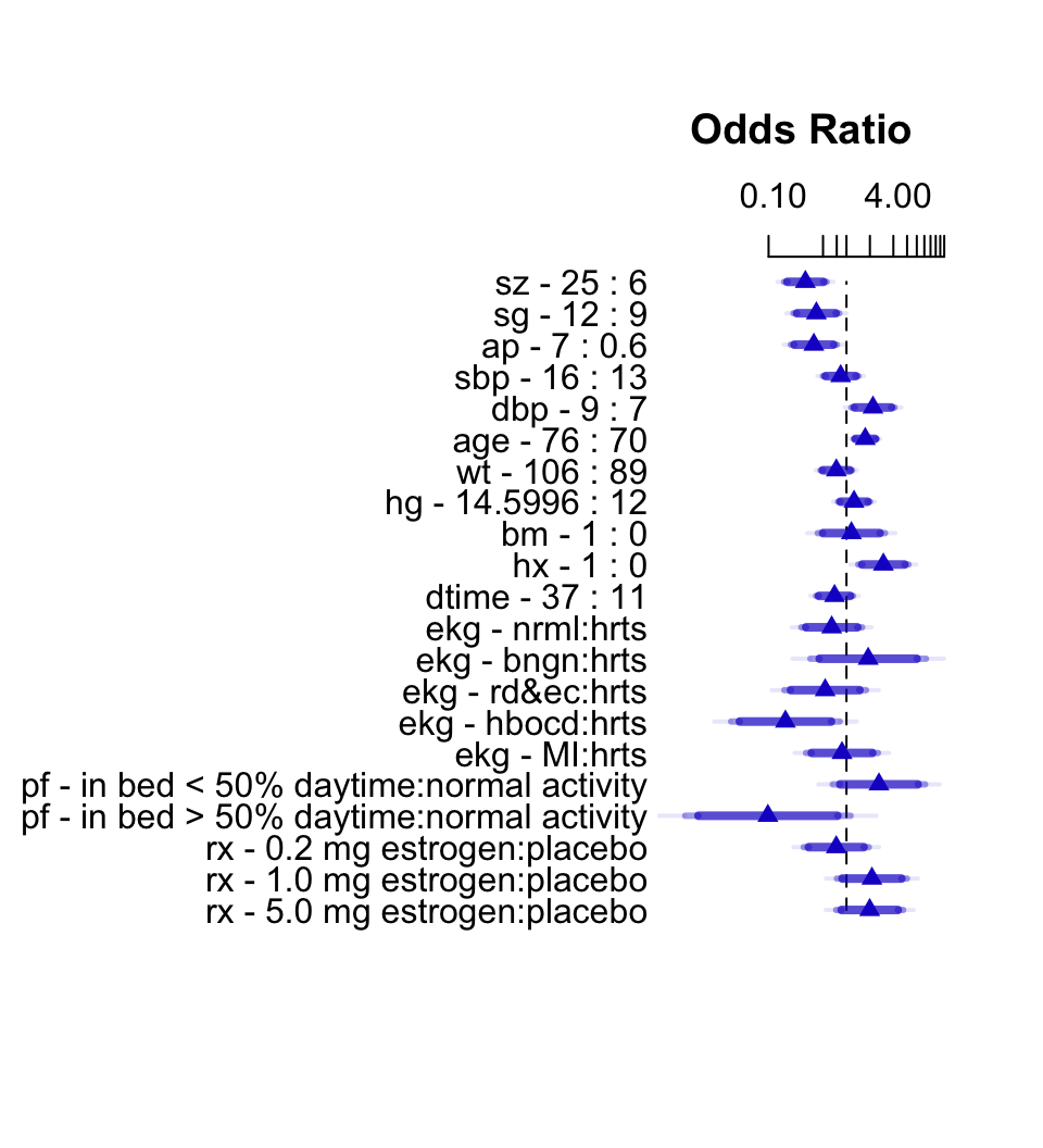
```{r h=5.5,w=5,top=2,cap='Interquartile-range odds ratios for continuous predictors and simple odds ratios for categorical predictors. Numbers at left are upper quartile : lower quartile or current group : reference group. The bars represent $0.9, 0.95, 0.99$ confidence limits. The intervals are drawn on the log odds ratio scale and labeled on the odds ratio scale. Ranges are on the original scale.',scap='Interquartile-range odds ratios and confidence limits'}
#| label: fig-lrcase1-fullor
plot(summary(f), log=TRUE)
```
The van Houwelingen--Le Cessie heuristic
shrinkage estimate (@eq-heuristic-shrink) is
$\hat{\gamma}=`r round(gamma.hat,2)`$, indicating that this model
will validate on new data about `r round(100*(1 - gamma.hat))`%
worse than on this dataset.
## Backwards Step-Down
Now use fast backward step-down (with total residual AIC as the stopping
rule) to identify the variables that explain the bulk of the cause of
death. Later validation will take this screening of variables into
account.
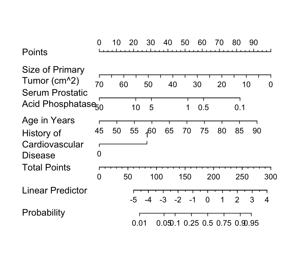
The greatly reduced model results in a simple nomogram.
```{r}
fastbw(f)
```
```{r}
fred <- lrm(cvd ~ sz + log(ap) + age + hx, data=psub)
latex(fred)
```
```{r w=5.5,h=5,ps=8,cap='Nomogram calculating $X\\hat{\\beta}$ and $\\hat{P}$ for `cvd` as the cause of death, using the step-down model. For each predictor, read the points assigned on the 0--100 scale and add these points. Read the result on the `Total Points` scale and then read the corresponding predictions below it.',scap='Nomogram for obtaining $X\\hat{\\beta}$ and $\\hat{P}$ from step-down model'}
#| label: fig-lrcase1-nom
nom <- nomogram(fred, ap=c(.1, .5, 1, 5, 10, 50),
                fun=plogis, funlabel="Probability",
                fun.at=c(.01,.05,.1,.25,.5,.75,.9,.95,.99))
plot(nom, xfrac=.45)
```
It is readily seen from this model that patients with a
history of heart disease, and patients with less extensive prostate cancer
are those more likely to die from `cvd` rather than from
cancer.
But beware that it is easy to over-interpret findings when using
unpenalized estimation, and confidence intervals are too
narrow. Let us use the bootstrap to study the uncertainty in the
selection of variables and to penalize for this uncertainty when
estimating predictive performance of the model. The variables
selected in the first 20 bootstrap resamples are shown, making it
obvious that the set of "significant" variables, i.e., the final
model, is somewhat arbitrary.
```{r results='hide'}
v <- validate(f, B=200, bw=TRUE)
```
```{r}
print(v, B=20, digits=3)
```
The slope shrinkage ($\hat{\gamma}$) is a bit lower than was estimated
above. There is drop-off in all indexes. The estimated likely future
predictive discrimination of the model as measured by Somers' $D_{xy}$
fell from `r round(v['Dxy','index.orig'],3)` to
`r round(v['Dxy','index.corrected'],3)`. The latter estimate is
the one that should be claimed when describing model performance.
A nearly unbiased estimate of future calibration of the
stepwise-derived model is given below.
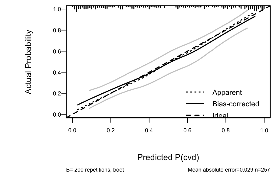
```{r h=3,w=4.75,cap='Bootstrap overfitting-corrected calibration curve estimate for the backwards step-down cause of death logistic model, along with a rug plot showing the distribution of predicted risks. The smooth nonparametric calibration estimator (`loess`) is used.',scap='Bootstrap nonparametric calibration curve for reduced cause of death model'}
#| label: fig-lrcase1-cal
spar(ps=9, bot=1)
cal <- calibrate(f, B=200, bw=TRUE)
plot(cal)
```
The amount of overfitting seen in @fig-lrcase1-cal is
consistent with the indexes produced by the `validate` function.
For comparison, consider a bootstrap validation of the full model
without using variable selection.
```{r}
vfull <- validate(f, B=200)
print(vfull, digits=3)
```
Compared to the validation of the full model, the step-down model
has less optimism, but it started with a smaller $D_{xy}$ due to
loss of information from removing moderately important variables. The
improvement
in optimism was not enough to offset the effect of eliminating variables.
If shrinkage were used with the full model, it would have better
calibration and discrimination than the reduced model, since shrinkage
does not diminish $D_{xy}$. Thus stepwise variable selection failed
at delivering excellent predictive discrimination.
Finally, compare previous results with a bootstrap validation of a
step-down model using a better significance level for a variable to
stay in the model ($\alpha=0.5$, @ste00pro) and using individual
approximate Wald tests rather than tests combining all deleted variables.
```{r}
v5 <- validate(f, bw=TRUE, sls=0.5, type='individual', B=200)
```
```{r}
print(v5, digits=3, B=0)
```
The performance statistics are midway between the full model and the
smaller stepwise model.
## Model Approximation {#sec-lrcase1-approx}
Frequently a better approach than stepwise variable selection is to
approximate the full model, using its estimates of precision, as
discussed in @sec-val-approx. Stepwise variable
selection as well as regression trees are useful for making the
approximations, and the sacrifice in predictive accuracy is always apparent.
We begin by computing the "gold standard" linear predictor from the
full model fit ($R^{2} = 1.0$), then running backwards step-down OLS
regression to approximate it.
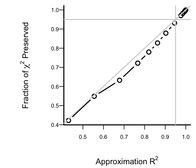
```{r h=3,w=3.5,cap='Fraction of explainable variation (full model LR $\\chi^2$) in `cvd` that was explained by approximate models, along with approximation accuracy ($x$-axis)',scap='Model approximation vs. LR $\\chi^2$ preserved'}
#| label: fig-lrcase1-approxr2
spar(bty='l', ps=9)
lp <- predict(f)   # Compute linear predictor from full model
# Insert sigma=1 as otherwise sigma=0 will cause problems
a <- ols(lp ~ sz + sg + log(ap) + sbp + dbp + age + wt +
         hg + ekg + pf + bm + hx + rx + dtime, sigma=1,
         data=psub)
# Specify silly stopping criterion to remove all variables
s <- fastbw(a, aics=10000)
betas <- s$Coefficients   # matrix, rows=iterations
X     <- cbind(1, f$x)    # design matrix
# Compute the series of approximations to lp
ap <- X %*% t(betas)
# For each approx. compute approximation R^2 and ratio of
# likelihood ratio chi-square for approximate model to that
# of original model
m <- ncol(ap) - 1   # all but intercept-only model
r2 <- frac <- numeric(m)
fullchisq <- f$stats['Model L.R.']
for(i in 1:m) {
  lpa <- ap[,i]
  r2[i] <- cor(lpa, lp)^2
  fapprox <- lrm(cvd ~ lpa, data=psub)
  frac[i] <- fapprox$stats['Model L.R.'] / fullchisq
  }
plot(r2, frac, type='b',
     xlab=expression(paste('Approximation ', R^2)),
     ylab=expression(paste('Fraction of ',
         chi^2, ' Preserved')))
abline(h=.95, col=gray(.83)); abline(v=.95, col=gray(.83))
abline(a=0, b=1, col=gray(.83))
```
After 6 deletions, slightly more than 0.05 of both the LR $\chi^2$ and
the approximation $R^2$ are
lost. Therefore we take as our
approximate model the one that removed 6 predictors. The equation for
this model is below, and its nomogram is in the figure below.
```{r}
fapprox <- ols(lp ~ sz + sg + log(ap) + age + ekg + pf + hx +
               rx, data=psub)
fapprox$stats['R2']   # as a check
latex(fapprox)
```
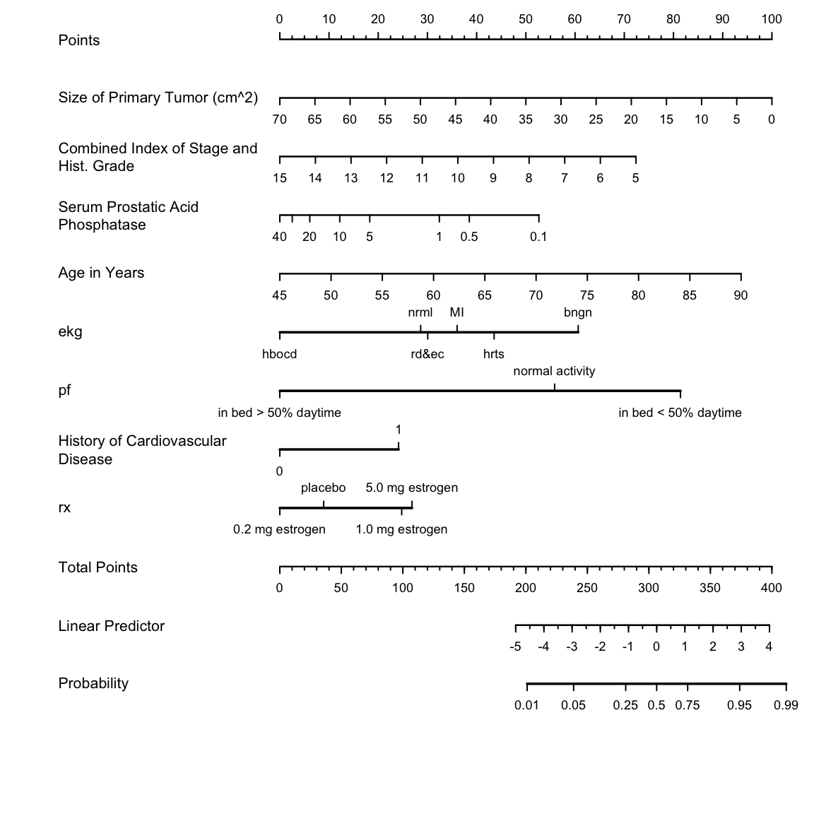
```{r h=6,w=6,cap='Nomogram for predicting the probability of `cvd` based on the approximate model',scap='Approximate nomogram for predicting cause of death'}
#| label: fig-lrcase1-nomapprox
spar(ps=8)
nom <- nomogram(fapprox, ap=c(.1, .5, 1, 5, 10, 20, 30, 40),
                fun=plogis, funlabel="Probability",
                lp.at=(-5):4,
           fun.lp.at=qlogis(c(.01,.05,.25,.5,.75,.95,.99)))
plot(nom, xfrac=.45)
```
```{r echo=FALSE}
saveCap('11')
```