```{r include=FALSE}
require(Hmisc)
options(qproject='rms', prType='html')
require(qreport)
getRs('qbookfun.r')
hookaddcap()
knitr::set_alias(w = 'fig.width', h = 'fig.height', cap = 'fig.cap', scap ='fig.scap')
```
# Ordinal Logistic Regression {#sec-ordinal}
**Resources**: [fharrell.com/post/rpo](https://fharrell.com/post/rpo)
## Background
`r mrg(sound("olr-1"))`
* Levels of $Y$ are ordered; no spacing assumed `r ipacue()`
* If no model assumed, one can still assess association between
$X$ and $Y$
* Example: $Y=0,1,2$ corresponds to no event, heart attack,
death. Test of association between race (3 levels) and outcome (3
levels) can be obtained from a $2 \times 2$ d.f. $\chi^2$ test for
a contingency table
* If willing to assuming an ordering of $Y$ _and_ a model,
can test for association using $2 \times 1$ d.f.
* Proportional odds model: generalization of
Wilcoxon-Mann-Whitney-Kruskal-Wallis-Spearman
* Can have $n$ categories for $n$ observations!
* Continuation ratio model: discrete proportional hazards model
* Ordinal models are _semiparametric_, i.e., distribution-free on the left-hand-side and parametric on the right hand $X\beta$ side of the model
## Ordinality Assumption {#sec-ordinal-ordinality}
A backwards way to look at ordinality ---
* Assume $X$ is linearly related to some appropriate log odds `r ipacue()`
* Estimate mean $X | Y$ with and without assuming the model holds
* For simplicity assume $X$ discrete
* Let $P_{jx} = \Pr(Y=j | X=x, model)$
\begin{array}{ccc}
\Pr(X=x | Y=j) &=& \Pr(Y=j | X=x) \frac{\Pr(X=x)}{\Pr(Y=j)} \nonumber \\
E(X | Y=j) &=& \sum_{x} x P_{jx} \frac{\Pr(X=x)}{\Pr(Y=j)} ,
\end{array}
and the expectation can be estimated by
$$
\hat{E}(X | Y=j) = \sum_{x} x \hat{P}_{jx} f_{x} / g_{j},
$$
where $\hat{P}_{jx}$ = estimate of $P_{jx}$ from the 1-predictor model
$$
\hat{E}(X | Y=j) = \sum_{i=1}^{n} x_{i} \hat{P}_{jx_{i}} / g_{j} .
$$
## Proportional Odds Model
`r mrg(sound("olr-2"))`
### Model
* @wal67est --- most popular ordinal response `r ipacue()`
model
* For convenience $Y=0, 1, 2, \ldots, k$
$$
\Pr[Y \geq j | X] = \frac{1}{1 + \exp[-(\alpha_{j} + X\beta)]} = \text{expit}(\alpha_{j} + X\beta)
$$
where $j=1, 2, \ldots, k$.
* $\alpha_j$ is the logit of Prob$[Y \geq j]$ when all $X$s are zero
* Odds $Y \geq j | X = \exp(\alpha_{j}+X\beta)$
* Odds $Y \geq j | X_{m}=a+1$ / Odds $Y \geq j | X_{m}=a = e^{\beta_{m}}$
* Same odds ratio $e^{\beta_{m}}$ for any $j=1,2,\ldots,k$
* Odds$[Y \geq j | X]$ / Odds$[Y \geq v | X] =
\frac{e^{\alpha_{j}+X\beta}}{e^{\alpha_{v}+X\beta}} =
e^{\alpha_{j}-\alpha_{v}}$
* Odds $Y \geq j | X$ = constant $\times$ Odds $Y \geq v | X$
* Assumes OR for 1 unit increase in age is the same when
considering the probability of death as when considering the
probability of death or heart attack
* PO model only uses ranks of $Y$; same $\hat{\beta}$s if
transform $Y$; is robust to outliers
## Assumptions and Interpretation of Parameters
### Estimation
### Residuals
* Construct binary events $Y\geq j, j=1,2,\ldots,k$ and use `r ipacue()`
corresponding predicted probabilities
$$
\hat{P}_{ij} = \text{expit}(\hat{\alpha}_{j}+X_{i}\hat{\beta}),
$$
* Score residual for subject $i$ predictor $m$:
$$
U_{im} = X_{im} ( [Y_{i}\geq j] - \hat{P}_{ij} ),
$$
* For each column of $U$ plot mean $\bar{U}_{\cdot m}$ and C.L.\
against $Y$
* Score residuals are not as useful in general semiparametric models for continuous $Y$ as they are in the Cox proportional hazards model
* Partial residuals may be more useful as they can also estimate
covariable transformations[@lan84gra; @col02mod]:
$$
r_{im} = \hat{\beta}_{m}X_{im} + \frac{Y_{i} - \hat{P}_{i}}{\hat{P}_{i}
(1 - \hat{P_{i}})},
$$
where
$$
\hat{P_{i}} = \frac{1}{1 + \exp[-(\alpha + X_{i}\hat{\beta})]} = \text{expit}(\alpha + X_{i}\hat{\beta}).
$$
* Smooth $r_{im}$ vs. $X_{im}$ to estimate how $X_{m}$ relates to
the log relative odds that $Y=1 | X_{m}$
* For ordinal $Y$ compute binary model partial res. for all
cutoffs $j$:
$$
r_{im} = \hat{\beta}_{m}X_{im} + \frac{ [Y_{i} \geq j] - \hat{P}_{ij}}{\hat{P}_{ij}
(1 - \hat{P}_{ij})},
$$
@li12new have a residual for ordinal models that
serves for the entire range of $Y$ without the need to consider
cutoffs. Their residual is useful for checking functional form of
predictors but not the proportional odds assumption.
### Assessment of Model Fit
`r ipacue()`
* @sec-ordinal-ordinality
* Stratified proportions $Y \geq j, j = 1, 2, \ldots, k$, since
$\text{logit}(Y \geq j | X) - \text{logit}(Y \geq i | X) = \alpha_{j} - \alpha_{i}$, for any constant $X$
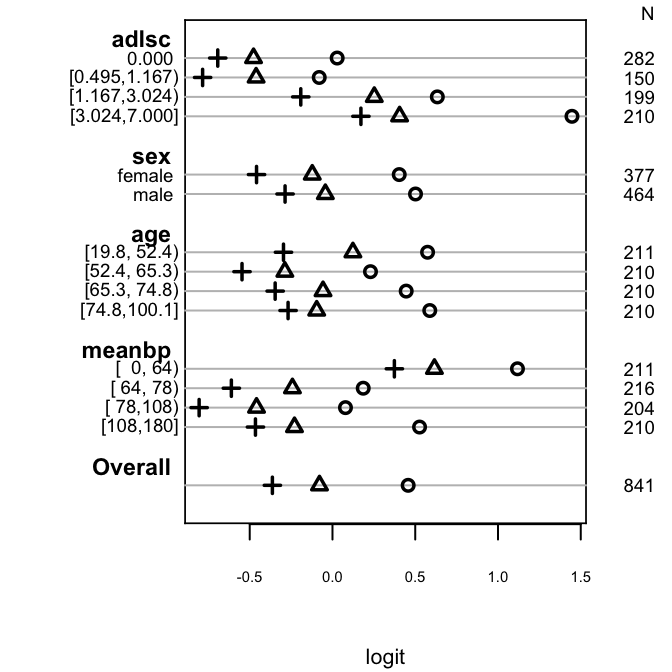
```{r po-assumpts-support,h=3.5,w=3.5,cap='Checking PO assumption separately for a series of predictors. The circle, triangle, and plus sign correspond to $Y \\geq 1, 2, 3$, respectively. PO is checked by examining the vertical constancy of distances between any two of these three symbols. Response variable is the severe functional disability scale `sfdm2` from the $1000$-patient SUPPORT dataset, with the last two categories combined because of low frequency of coma/intubation.',scap='Simple method for checking PO assumption using stratification'}
#| label: fig-ordinal-po-assumpts-support
spar(ps=7)
require(Hmisc)
getHdata(support)
sfdm <- as.integer(support$sfdm2) - 1
sf <- function(y)
  c('Y>=1'=qlogis(mean(y >= 1)), 'Y>=2'=qlogis(mean(y >= 2)),
    'Y>=3'=qlogis(mean(y >= 3)))
s <- summary(sfdm ~ adlsc + sex + age + meanbp, fun=sf, data=support)
plot(s, which=1:3, pch=1:3, xlab='logit', vnames='names', main='',
     width.factor=1.5)
```
<!-- %NEW 2022-03-01--->
Note that computing ORs for various cutoffs and seeing disagreements among them can cause reviewers to confuse lack of fit with sampling variation (random chance). For a 4-level Y having a given vector of probabilities in a control group, let's assume PO with a true OR of 3 and simulate 10 experiments to show variation of observed ORs over all cutoffs of Y. First do it for a sample size of n=10,000 then for n=200.
```{r randomor}
p <- c(.1, .2, .3, .4)
set.seed(7)
simPOcuts(10000, odds.ratio=3, p=p)
simPOcuts( 200, odds.ratio=3, p=p)
```
A better approach for discrete Y is to show the
_impact_ of making the PO assumption:
* Select a set of covariate settings over which to evaluate `r ipacue()`
accuracy of predictions
* Vary at least one of the predictors, i.e., the one for which you
want to assess the impact of the PO assumption
* Fit a PO model the usual way
* Fit other models that relax the PO assumption
+ to relax the PO assumption for all predictors fit a
multinomial logistic model
+ to relax the PO assumption for a subset of predictors fit a
partial PO model [@pet90par] (here using the `R` `VGAM` function)
* For all the covariate combinations evaluate predicted
probabilities for all levels of Y using the PO model and the relaxed
assumption models
* Use the bootstrap to compute confidence intervals for the
difference in predicted probabilities between a PO and a relaxed
model. This guards against over-emphasis of differences when the
sample size does not support estimation, especially for the relaxed
model with more parameters. Note that the sample problem occurs
when comparing predicted unadjusted probabilities to observed
proportions, as observed proportions can be noisy.
Example: re-do the assessment above. Note that the `VGAM` package `vglm` function did not converge when fitting the partial proportional odds model. So in what follows we only compare the fully PO model with the fully non-PO multinomial model.
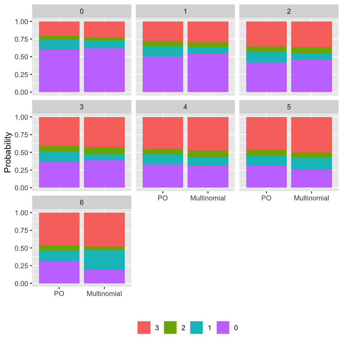
```{r po-assumpts-impact,h=6,w=6,cap='Checking the impact of the PO assumption by comparing predicted probabilities of all outcome categories from a PO model with a multinomial logistic model that assumes PO for no variables',scap='Checking impact of the PO assumption'}
#| label: fig-ordinal-po-assumpts-impact
spar(ps=7)
require(rms)
require(ggplot2)
# One headache: since using a non-rms fitting function need to hard
# code knots in splines.  This is not necessary in rms 6.5-0 and later
kq   <- seq(0.05, 0.95, length=4)
kage <- quantile(support$age,    kq, na.rm=TRUE)
kbp  <- quantile(support$meanbp, kq, na.rm=TRUE)

d    <- expand.grid(adlsc=0:6, sex='male', age=65, meanbp=78)

# Because of very low frequency (7) of sfdm=3, combine categories 3, 4
support$sfdm3 <- pmin(sfdm, 3)

done.impact <- TRUE
if(done.impact) w <- readRDS('impactPO.rds') else {
  set.seed(1)
  w <- impactPO(sfdm3 ~ pol(adlsc, 2) + sex + rcs(age, kage) +
                  rcs(meanbp, kbp),
                newdata=d, B=300, data=support)
  saveRDS(w, 'impactPO.rds')
}
w
# Reverse levels of y so stacked bars have higher y located higher
revo <- function(z) {
  z <- as.factor(z)
  factor(z, levels=rev(levels(as.factor(z))))
}
ggplot(w$estimates, aes(x=method, y=Probability, fill=revo(y))) +
    facet_wrap(~ adlsc) + geom_col() +
    xlab('') + guides(fill=guide_legend(title='')) +
    theme(legend.position='bottom')
```
AIC indicates that a model assuming PO nowhere is better than
one that assumes PO everywhere. In an earlier run in which convergence was obtained using `vglm`, the PPO model with far fewer
parameters is just as good, and is also better than the PO model,
indicating non-PO with respect to `adlsc`.
The fit of the PO model is such that cell probabilities become more
inaccurate for higher level outcomes. This can also be seen by the
increasing mean absolute differences with probability estimates from
the PO model. Bootstrap nonparametric percentile confidence intervals
(300 resamples, not all of which converged)
for differences in predicted cell probabilities between the PO model
and a relaxed model are also found above. Some of these intervals
exclude 0, in line with the other evidence for non-PO.
See
[fharrell.com/post/impactpo](https://fharrell.com/post/impactpo)
for a similar example.
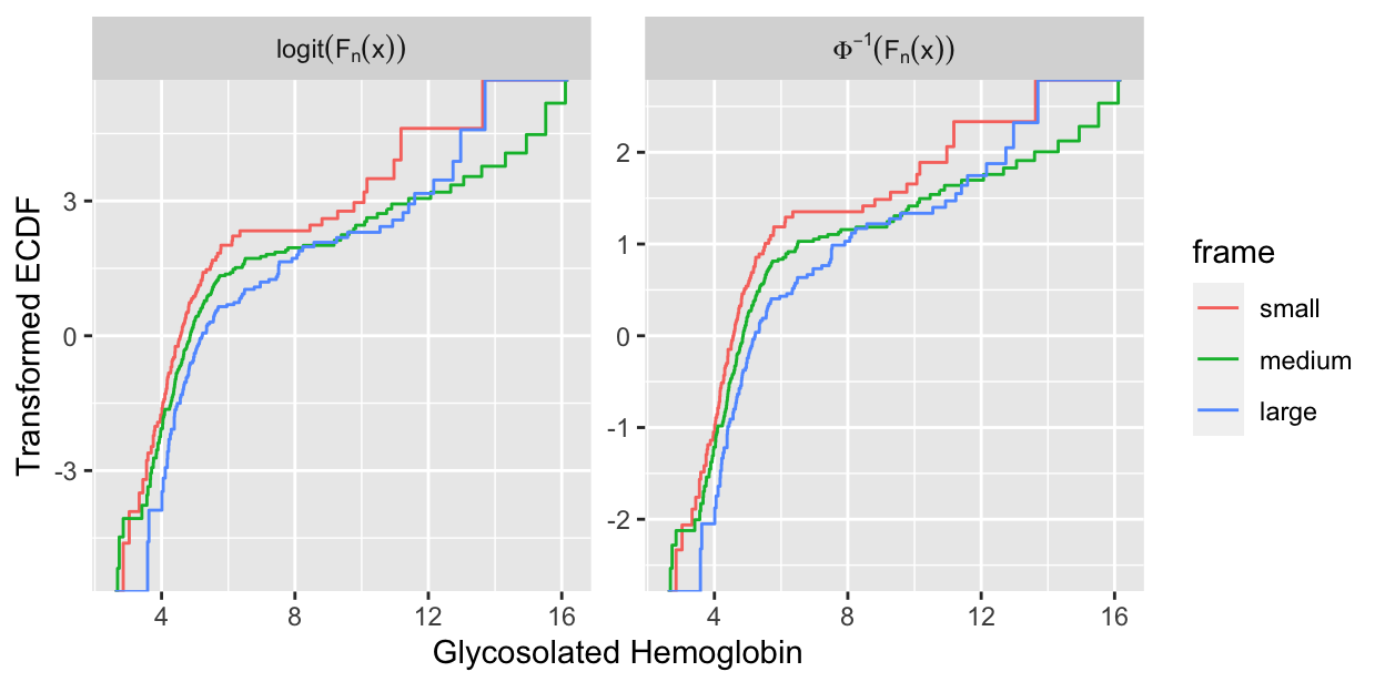
When $Y$ is continuous or almost continuous and $X$ is discrete, the
PO model assumes that the logit of the cumulative distribution
function of $Y$ is parallel across categories of $X$.
The corresponding, more rigid, assumptions of the ordinary linear
model (here, parametric ANOVA) are parallelism and linearity of the
normal inverse cumulative
distribution function across categories of $X$. As an example
consider the web site's `diabetes` dataset, where we consider the
distribution of log glycohemoglobin across subjects' body frames.
```{r glyhb,h=3.25,w=6.5,cap='Transformed empirical cumulative distribution functions stratified by body frame in the `diabetes` dataset. Left panel: checking all assumptions of the parametric ANOVA. Right panel: checking all assumptions of the PO model (here, Kruskal--Wallis test).',scap='Checking assumptions of PO and parametric model'}
#| label: fig-ordinal-glyhb
require(data.table)
getHdata(diabetes)
d <- subset(diabetes, ! is.na(frame))
setDT(d)  # make it a data table
w <- d[, ecdfSteps(glyhb, extend=c(2.6, 16.2)), by=frame]
# ecdfSteps is in Hmisc
# Duplicate ECDF points for trying 2 transformations
u <- rbind(data.table(trans='paste(Phi^-1, (F[n](x)))', w[, z := qnorm(y) ]),
           data.table(trans='logit(F[n](x))',           w[, z := qlogis(y)]))
# See https://hbiostat.org/rflow/graphics.html#sec-graphics-ggplot2
ggplot(u, aes(x, z, color=frame)) + geom_step() +
  facet_wrap(~ trans, label='label_parsed', scale='free_y') +
  ylab('Transformed ECDF') +
  xlab(hlab(glyhb))   # hlab is in Hmisc; looks up label in d
```
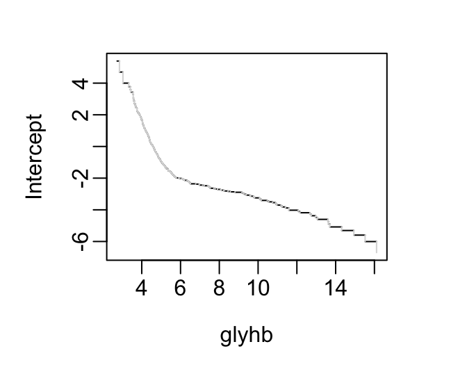
See how these distributions are reflected in proportional odds model intercepts.
```{r ints}
#| fig-height: 2.75
#| fig-width: 3.5
f <- orm(glyhb ~ frame, data=d)
plotIntercepts(f)
```
<!-- NEW -->
Especially for continuous predictors, the `rms` package `ordParallel` provides graphical and formal assessments of proportionality (adequacy of link). See @sec-cony for an example.
### Quantifying Predictive Ability
### Describing the Model
For PO models there are four and sometimes five types of
relevant predictions:
1. logit$[Y \geq j | X]$, i.e., the linear predictor `r ipacue()`
1. Prob$[Y \geq j | X]$
1. Prob$[Y = j | X]$
1. Quantiles of $Y | X$ (e.g., the median^[If $Y$ does not have very many levels, the median will be a discontinuous function of $X$ and may not be satisfactory.])
1. $E(Y | X)$ if $Y$ is interval scaled.
Graphics:
1. Partial effect plot (prob. scale or mean) `r ipacue()`
1. Odds ratio chart
1. Nomogram (possibly including the mean)
### Validating the Fitted Model
### `R` Functions
`r mrg(sound("olr-3"))`
The `rms` package's `lrm` and `orm` functions fit the PO model
directly, assuming that the levels of the response variable (e.g., the
`levels` of a `factor` variable) are listed in the proper
order. `predict` computes all types of estimates except for quantiles.
`orm` allows for more link functions than the logistic and is
intended to efficiently handle hundreds of intercepts as happens when
$Y$ is continuous.
The `R` functions `popower` and `posamsize` (in the
`Hmisc` package) compute power and sample size estimates for
ordinal responses using the proportional odds model.
The function `plot.xmean.ordinaly` in `rms` computes and graphs the
quantities described in @sec-ordinal-ordinality. It plots
simple $Y$-stratified means overlaid with $\hat{E}(X | Y=j)$, with
$j$ on the $x$-axis. The $\hat{E}$s are computed for both PO and
continuation ratio ordinal logistic models.
The `Hmisc` package's `summary.formula` function is also useful
for assessing the PO assumption.
Generic `rms` functions such as `validate`, `calibrate`,
and `nomogram` work with PO model fits from `lrm` as long as the
analyst specifies which intercept(s) to use.
`rms` has a special function generator `Mean` for
constructing an easy-to-use function for getting the predicted mean
$Y$ from a PO model. This is handy with `plot` and `nomogram`.
If the fit has been run through `bootcov`, it is easy to use the
`Predict` function to estimate bootstrap confidence limits for
predicted means.
## Continuation Ratio Model
`r mrg(sound("olr-4"))`
### Model
Unlike the PO model, which is based on _cumulative_ probabilities, the
continuation ratio (CR) model is based on _conditional_ probabilities.
The (forward) CR model[@fie07ana; @arm89ord; @ber91ana] is stated as follows
for $Y=0,\ldots,k$:
$$\begin{array}{c}
\Pr(Y=j | Y \geq j, X) &=& \text{expit}(\theta_{j} + X\gamma)
\nonumber \\
\text{logit}(Y=0 | Y \geq 0, X) &=& \text{logit}(Y=0 | X) \nonumber \\
&=& \theta_{0} + X\gamma \\
\text{logit}(Y=1 | Y \geq 1, X) &=& \theta_{1} + X\gamma \nonumber \\
\ldots & & \nonumber \\
\text{logit}(Y=k-1 | Y \geq k-1, X) &=& \theta_{k-1} + X\gamma . \nonumber
\end{array}$$ {#eq-cr-equation}
The CR model has been said to be likely to fit ordinal responses when
subjects have to "pass through" one category to get to the next
The CR model is a discrete version of the Cox proportional hazards
model. The discrete hazard function is defined as $\Pr(Y=j | Y \geq j)$.
Advantage of CR model: easy to allow unequal slopes across $Y$ for
selected $X$.
### Assumptions and Interpretation of Parameters
### Estimation
### Residuals
To check CR model assumptions, binary logistic model partial residuals
are again valuable. We separately fit a sequence of binary logistic
models using a series of binary events and the corresponding
applicable (increasingly small) subsets of subjects, and plot smoothed partial
residuals against $X$ for all of the binary events. Parallelism in
these plots indicates that the CR model's constant $\gamma$
assumptions are satisfied.
### Assessment of Model Fit
### Extended CR Model
### Role of Penalization in Extended CR Model
### Validating the Fitted Model
### `R` Functions
The `cr.setup` function in `rms` returns a list of vectors
useful in constructing a dataset used to trick a binary logistic
function such as `lrm` into fitting CR models.
```{r echo=FALSE}
saveCap('13')
```