```{r include=FALSE}
require(Hmisc)
require(qreport)
options(qproject='rms', prType='html')
getRs('qbookfun.r')
hookaddcap()
knitr::set_alias(w = 'fig.width', h = 'fig.height', cap = 'fig.cap', scap ='fig.scap')
```
# Logistic Model Case Study: Survival of Titanic Passengers {#sec-titanic}
`r mrg(sound("titanic-1"))`
**Data source**: _The Titanic Passenger List_ edited by
Michael A. Findlay, originally published in Eaton \& Haas (1994) _Titanic: Triumph and Tragedy_, Patrick Stephens Ltd, and expanded with
the help of the Internet community. The original `html` files were
obtained from [Philip Hind (1999)](http://atschool.eduweb.co.uk/phind). The dataset was
compiled and interpreted by Thomas Cason. It is available in `R` and
spreadsheet formats from [hbiostat.org/data](https://hbiostat.org/data) under the name `titanic3`.
## Descriptive Statistics
```{r desc}
require(rms)
options(prType='html')   # for print, summary, anova
getHdata(titanic3)        # get dataset from web site
# List of names of variables to analyze
v <- c('pclass','survived','age','sex','sibsp','parch')
t3 <- titanic3[, v]
units(t3$age) <- 'years'
describe(t3)
```
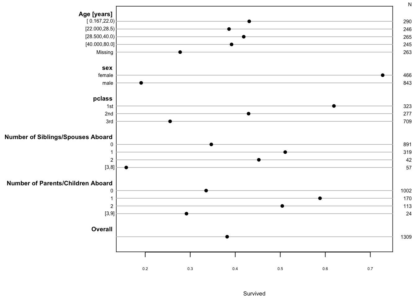
```{r summary,cap='Univariable summaries of Titanic survival'}
#| label: fig-titanic-summary
spar(ps=6,rt=3)
dd <- datadist(t3)
# describe distributions of variables to rms
options(datadist='dd')
s <- summary(survived ~ age + sex + pclass +
             cut2(sibsp,0:3) + cut2(parch,0:3), data=t3)
plot(s, main='', subtitles=FALSE)
```
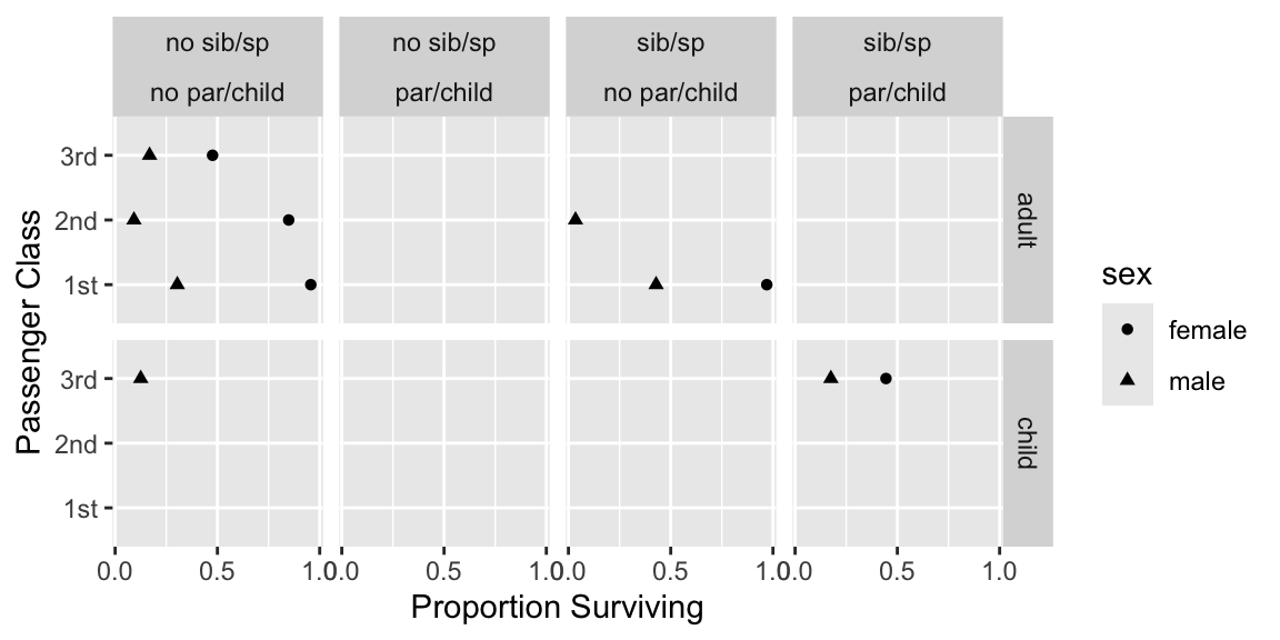
Show 4-way relationships after collapsing levels. Suppress estimates `r ipacue()` based on $<25$ passengers.
```{r dot,h=3,w=6,cap='Multi-way summary of Titanic survival'}
#| label: fig-titanic-dot
require(ggplot2)
tn <- transform(t3,
  agec = ifelse(age < 21, 'child', 'adult'),
  sibsp= ifelse(sibsp == 0, 'no sib/sp', 'sib/sp'),
  parch= ifelse(parch == 0, 'no par/child', 'par/child'))
g <- function(y) if(length(y) < 25) NA else mean(y)
s <- with(tn, summarize(survived,
           llist(agec, sex, pclass, sibsp, parch), g))
# llist, summarize in Hmisc package
ggplot(subset(s, agec != 'NA'),
  aes(x=survived, y=pclass, shape=sex)) +
  geom_point() + facet_grid(agec ~ sibsp * parch) +
  xlab('Proportion Surviving') + ylab('Passenger Class') +
  scale_x_continuous(breaks=c(0, .5, 1))
```
## Exploring Trends with Nonparametric Regression
`r mrg(sound("titanic-2"))`
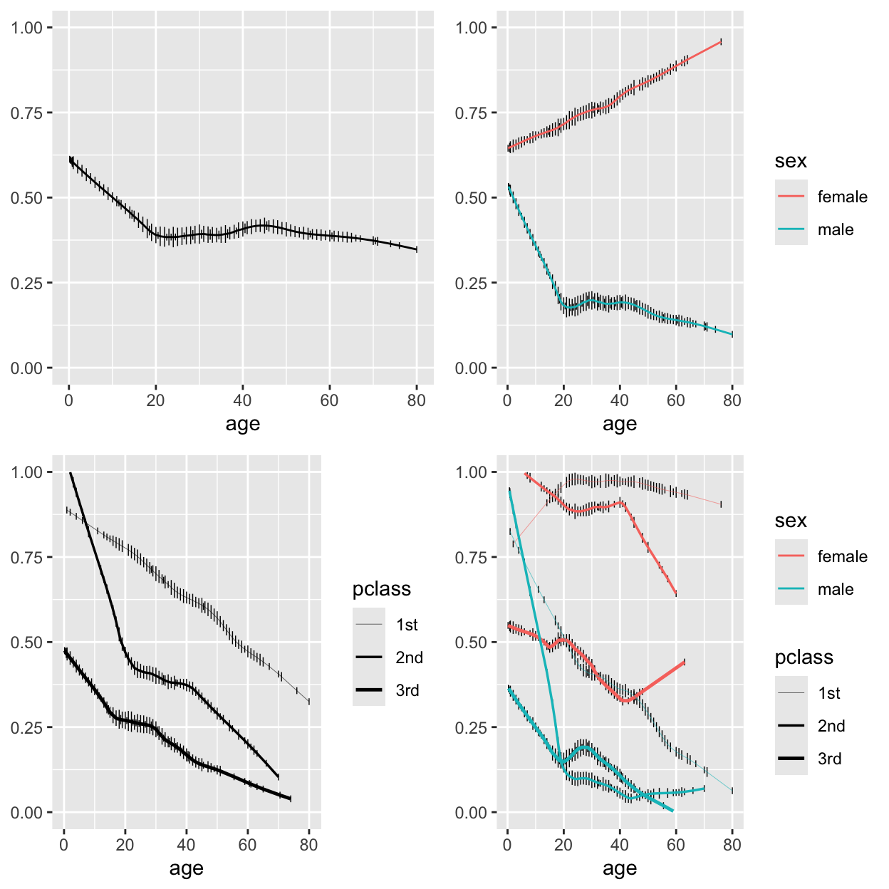
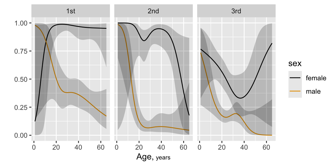
```{r plsmoa,h=6.5,w=6.5,cap='Nonparametric regression (`loess`) estimates of the relationship between age and the probability of surviving the Titanic, with tick marks depicting the age distribution. The top left panel shows unstratified estimates of the probability of survival. Other panels show nonparametric estimates by various stratifications.',scap='Nonparametric regression for age, sex, class, and passenger survival'}
#| label: fig-titanic-plsmoa
b  <- scale_size_discrete(range=c(.1, .85))
yl <- ylab(NULL)
p1 <- ggplot(t3, aes(x=age, y=survived)) +
      histSpikeg(survived ~ age, lowess=TRUE, data=t3) +
      ylim(0,1) + yl
p2 <- ggplot(t3, aes(x=age, y=survived, color=sex)) +
      histSpikeg(survived ~ age + sex, lowess=TRUE,
                 data=t3) + ylim(0,1) + yl
p3 <- ggplot(t3, aes(x=age, y=survived, size=pclass)) +
      histSpikeg(survived ~ age + pclass, lowess=TRUE,
                 data=t3) + b + ylim(0,1) + yl
p4 <- ggplot(t3, aes(x=age, y=survived, color=sex,
       size=pclass)) +
      histSpikeg(survived ~ age + sex + pclass,
                 lowess=TRUE, data=t3) +
      b + ylim(0,1) + yl
gridExtra::grid.arrange(p1, p2, p3, p4, ncol=2)   # combine 4
```
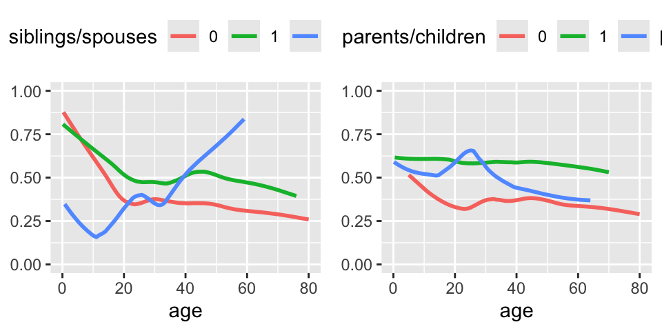
```{r plsmob, w=5, h=2.5,cap='Relationship between age and survival stratified by the number of siblings or spouses on board (left panel) or by the number of parents or children of the passenger on board (right panel).',scap='Relationship between age and survival stratified by family size variables'}
#| label: fig-titanic-plsmob
top <- theme(legend.position='top')
p1 <- ggplot(t3, aes(x=age, y=survived, color=cut2(sibsp,
       0:2))) + stat_plsmo() + b + ylim(0,1) + yl + top +
      scale_color_discrete(name='siblings/spouses')
p2 <- ggplot(t3, aes(x=age, y=survived, color=cut2(parch,
       0:2))) + stat_plsmo() + b + ylim(0,1) + yl + top +
      scale_color_discrete(name='parents/children')
gridExtra::grid.arrange(p1, p2, ncol=2)
```
## Binary Logistic Model with Casewise Deletion of Missing Values {#sec-titanic-cd}
`r mrg(sound("titanic-3"))`
<!-- NEW -->
* First fit a model that is saturated with respect to `age, sex, pclass`
* Insufficient variation in `sibsp`, `parch` to fit complex interactions or nonlinearities.
* With `age` appearing in so many terms, giving too many parameters to `age` creates instabilities and makes many bootstrap repetitions fail to converge or to yield singular covariance matrices
* Use AIC to determine the global number of knots for `age` that is "best for the money" in terms of being the most likely to cross-validate well
```{r anova3}
for(k in 3 : 5) {
  f <- lrm(survived ~ sex*pclass*rcs(age, k) +
           rcs(age, k)*(sibsp + parch), data=t3)
  cat('k=', k, '  AIC=', AIC(f), '\n')
}
```
* 4 knots has best (lowest) AIC and we'll use that going forward
* Refit that model with x=TRUE, y=TRUE so can do likelihood ratio (LR) tests
* But start with Wald tests
```{r}
f1 <- lrm(survived ~ sex*pclass*rcs(age,4) +
          rcs(age,4)*(sibsp + parch), data=t3, x=TRUE, y=TRUE)
print(f1, r2=1:4)   # print all 4 R^2 measures that use only the global LR chi-square
anova(f1)
```
Compute the slightly more time-consuming LR tests
```{r}
af1 <- anova(f1, test='LR')
print(af1, which='subscripts')
```
* In the RMS text, 5 knots were used for `age` and only Wald tests were performed
* Large $p$-value for the 3rd order interaction was used to justify exclusion of these highest-order interactions from the model (and one other term)
* More evidence for 3rd order interaction from the more accurate LR test
* Keep this model
Show the many effects of predictors. `r ipacue()`
```{r plot1, h=3, w=6, cap='Effects of predictors on probability of survival of Titanic passengers, estimated for zero siblings/spouses and zero parents/children',scap='Effects of predictors on probability of surviving the Titanic'}
#| label: fig-titanic-plota
p <- Predict(f1, age, sex, pclass, sibsp=0, parch=0, fun=plogis)
ggplot(p)
```
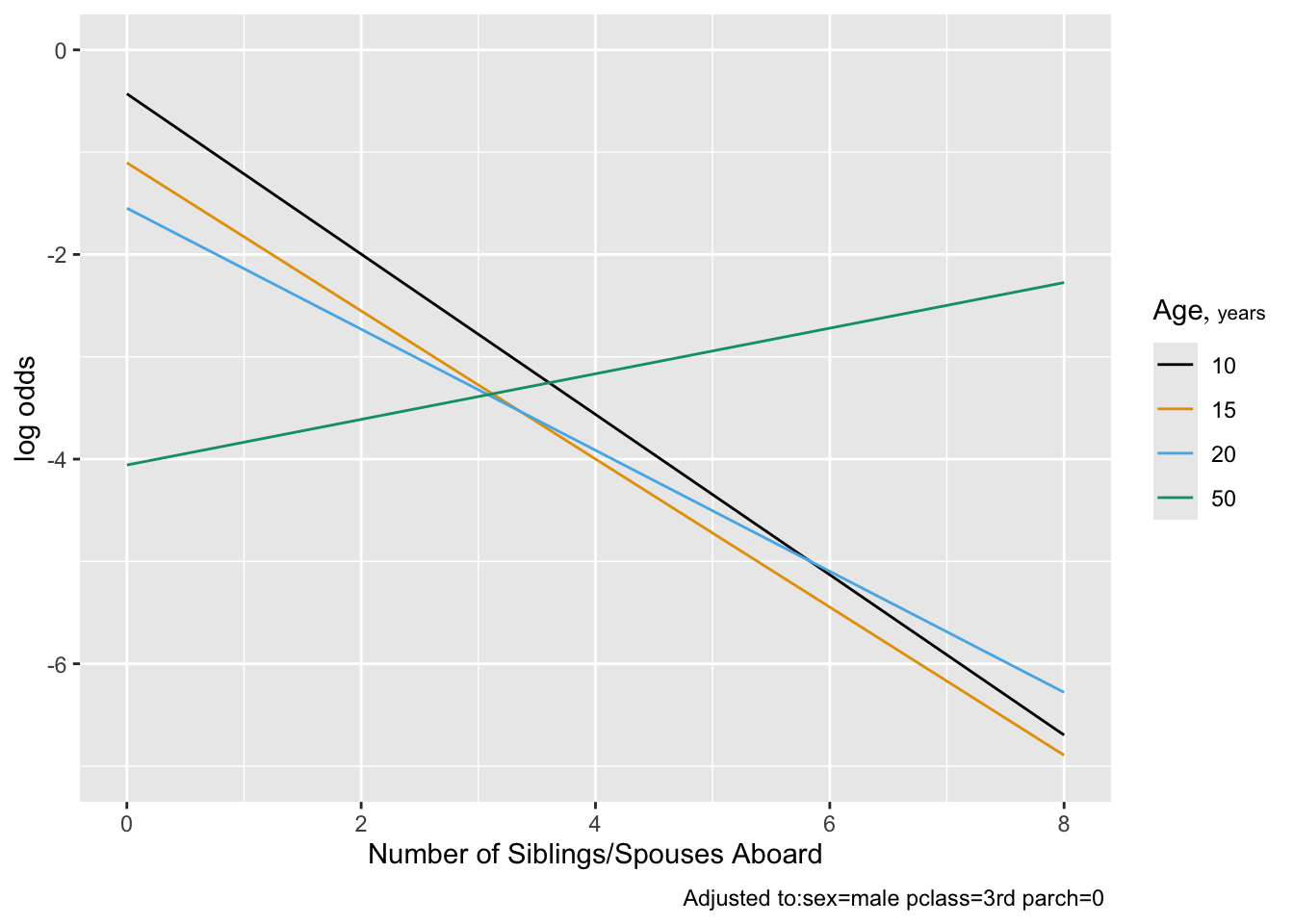
```{r plot2,cap='Effect of number of siblings and spouses on the log odds of surviving, for third class males',scap='Effect of number of siblings/spouses on survival'}
#| label: fig-titanic-plotb
ggplot(Predict(f1, sibsp, age=c(10,15,20,50), conf.int=FALSE))
#
```
Note that children having many siblings apparently had lower
survival. Married adults had slightly higher survival than unmarried
ones.
`r ipacue()`
**But** moderate problem with missing data must be dealt with
## Examining Missing Data Patterns {#sec-titanic-naclus}
`r mrg(sound("titanic-4"))`
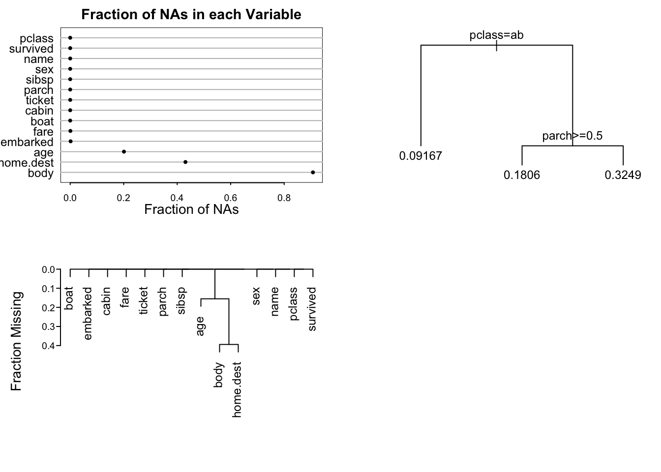
```{r napatterns,h=5,w=7,cap='Patterns of missing data. Upper left panel shows the fraction of observations missing on each predictor. Lower panel depicts a hierarchical cluster analysis of missingness combinations. The similarity measure shown on the $Y$-axis is the fraction of observations for which both variables are missing. Right panel shows the result of recursive partitioning for predicting `is.na(age)`. The `rpart` function found only strong patterns according to passenger class.',scap='Patterns of missing Titanic data'}
#| label: fig-titanic-napatterns
spar(mfrow=c(2,2), top=1, ps=11)
na.patterns <- naclus(titanic3)
require(rpart)      # Recursive partitioning package
who.na <- rpart(is.na(age) ~ sex + pclass + survived +
                sibsp + parch, data=titanic3, minbucket=15)
naplot(na.patterns, 'na per var')
plot(who.na, margin=.1); text(who.na)
plot(na.patterns)
```
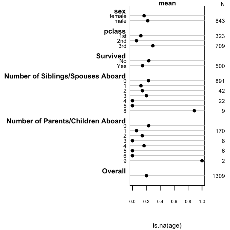
```{r summary-na,w=4,h=4,cap='Univariable descriptions of proportion of passengers with missing age'}
#| label: fig-titanic-summary-na
spar(ps=7, rt=3)
plot(summary(is.na(age) ~ sex + pclass + survived +
             sibsp + parch, data=t3))
```
But models almost always provide better descriptive statistics
```{r nalrm}
m <- lrm(is.na(age) ~ sex * pclass + survived + sibsp + parch,
         data=t3)
m
anova(m)
```
`pclass` and `parch` are the important predictors of missing age.
## Single Conditional Mean Imputation
Single imputation is not the preferred approach here. Click below to see this section.
::: {.callout-note collapse="true"}
### Single Imputation and Analysis Result
`r ipacue()`
First try: conditional mean imputation <br>
Default spline transformation for age caused distribution of
imputed values to be much different from non-imputed ones; constrain
to linear. Also force discrete numeric variables to be linear because knots are hard to determine for them.
```{r transcan}
xtrans <- transcan(~ I(age) + sex + pclass + I(sibsp) + I(parch),
                   imputed=TRUE, pl=FALSE, pr=FALSE, data=t3)
summary(xtrans)
# Look at mean imputed values by sex,pclass and observed means
# age.i is age, filled in with conditional mean estimates
age.i <- with(t3, impute(xtrans, age, data=t3))
i <- is.imputed(age.i)
with(t3, tapply(age.i[i], list(sex[i],pclass[i]), mean))
with(t3, tapply(age, list(sex,pclass), mean, na.rm=TRUE))
```
```{r fit.si}
dd   <- datadist(dd, age.i)
f.si <- lrm(survived ~ sex * pclass * rcs(age.i, 4) +
            rcs(age.i, 4) * (sibsp + parch), data=t3, x=TRUE, y=TRUE)
print(f.si, coefs=FALSE)
```
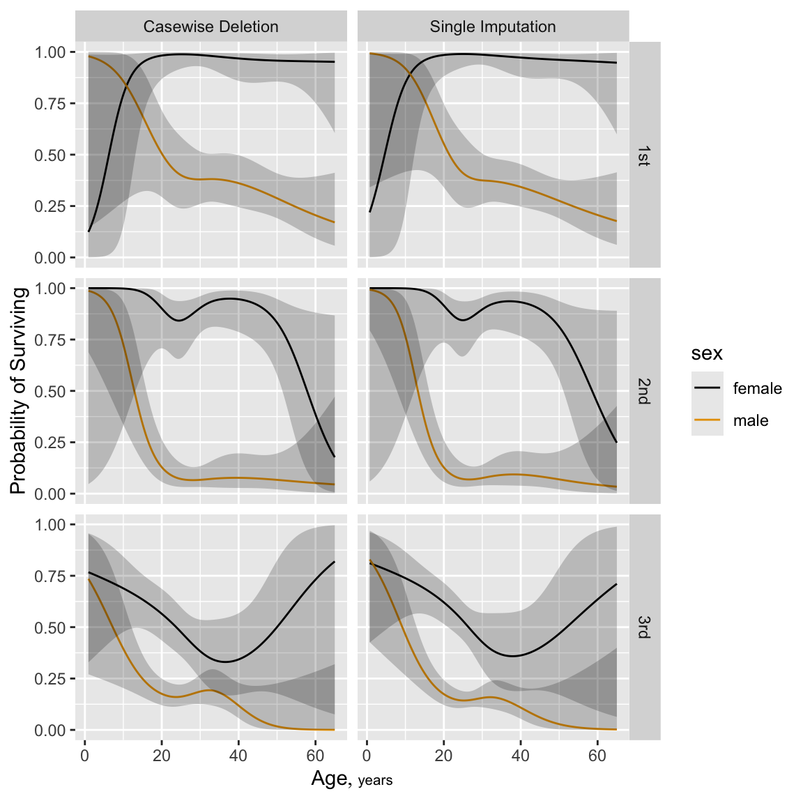
```{r h=6, w=6, cap='Predicted probability of survival for males from fit using casewise deletion (bottom) and single conditional mean imputation (top). `sibsp` is set to zero for these predicted values.',scap='Predicted log odds of survival in Titanic using casewise deletion'}
#| label: fig-titanic-nasingle
spar(ps=12)
p1 <- Predict(f1,   age,   pclass, sex, sibsp=0, fun=plogis)
p2 <- Predict(f.si, age.i, pclass, sex, sibsp=0, fun=plogis)
p  <- rbind('Casewise Deletion'=p1, 'Single Imputation'=p2,
            rename=c(age.i='age'))   # creates .set. variable
ggplot(p, groups='sex', ylab='Probability of Surviving')
anova(f.si, test='LR')
```
:::
## Multiple Imputation
`r mrg(sound("titanic-5"))`
The following uses `aregImpute` with predictive mean matching. By
default, `aregImpute` does not transform `age` when it is being
predicted from the other variables. Four knots are used to transform
`age` when used to impute other variables (not needed here as no
other missings were present). Since the fraction of observations with
missing age is $\frac{263}{1309} = 0.2$ we use 20 imputations. [Force `sibsp` and `parch` to be linear for imputation, because their highly discrete distributions make it difficult to choose knots for splines.]{.aside}
```{r aregi}
set.seed(17)         # so can reproduce random aspects
mi <- aregImpute(~ age + sex + pclass +
                 I(sibsp) + I(parch) + survived,
                 data=t3, n.impute=20, nk=4, pr=FALSE)
mi
# Print the first 10 imputations for the first 10 passengers
#  having missing age
mi$imputed$age[1:10, 1:10]
```
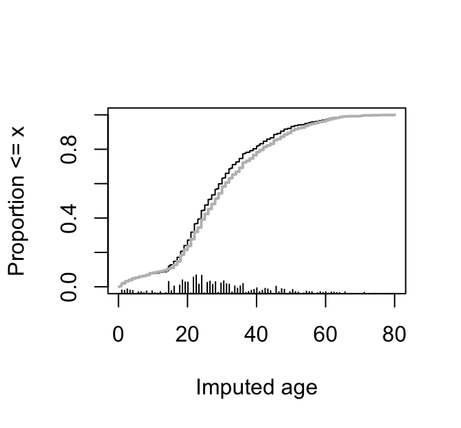
Show the distribution of imputed (black) and actual ages (gray). `r ipacue()`
```{r ageDist,w=3.5,h=3.25,cap='Distributions of imputed and actual ages for the Titanic dataset. Imputed values are in black and actual ages in gray.',scap='Distribution of imputed and actual ages'}
#| label: fig-titanic-agedist
plot(mi)
Ecdf(t3$age, add=TRUE, col='gray', lwd=2,
     subtitles=FALSE)
```
* Fit logistic models for 20 completed datasets and print the ratio `r ipacue()`
of imputation-corrected variances to average ordinary variances.
* Use method of [Chan & Meng](missing#lrt) to get LR tests
* This method takes final $\hat{\beta}$ from a single model fit on 20 stacked completed datasets
* But standard errors come from the usual Rubin's rule and the 20 fits
* `rms::processMI` computes the LR statistics from special information saved by `fit.mult.impute` triggered by `lrt=TRUE`
* The `Hmisc` package `runifChanged` function is used to save the result and not spend 1m running it again until an input changes
* The `rms` `LRupdate` function is run to fix likelihood ratio-related statistics (LR test, its $p$-value, various $R^2$ measures) using the overall Chan & Meng model LR $\chi^2$ computed by `processMI`
* Two of the $R^2$ printed use an effective sample size of 927 for the unbalanced binary `survived` variable
```{r fmi}
runmi <- function()
  fit.mult.impute(survived ~ sex * pclass * rcs(age, 4) + rcs(age, 4) * (sibsp + parch),
                  lrm, mi, data=t3, pr=FALSE, lrt=TRUE)  # lrt implies x=TRUE y=TRUE + more
seed <- 17
f.mi <- runifChanged(runmi, seed, mi, t3)
afmi <- processMI(f.mi, 'anova')
# Print imputation penalty indexes
prmiInfo(afmi)
```
* None of the denominator d.f. is small enough for us to worry about the $\chi^2$ approximation
* Take the ratio of selected LR statistics after multiple imputation to that from casewise deletion
```{r}
afmi
f.mi <- LRupdate(f.mi, afmi)
print(f.mi, r2=1:4)   # print all 4 imputation-adjusted R^2
round(afmi[c(1,3,5,30), 'Chi-Square'] / af1[c(1,3,5,30), 'Chi-Square'], 3)
```
`r ipacue()`
* Using all available data resulted in increases in predictive information for `sex, pclass` and strangely a reduction for `age`
For each completed dataset run bootstrap validation of model performance indexes and the nonparametric calibration curve. Because the 20 analyses of completed datasets help to average out some of the noise in bootstrap estimates we can use fewer bootstrap repetitions (100) than usual (300 or so).
```{r fmival}
val <- function(fit)
  list(validate  = validate (fit, B=100),
       calibrate = calibrate(fit, B=100) )

runmi <- function()
  fit.mult.impute(       # 1m
    survived ~ sex * pclass * rcs(age,4) +
    rcs(age,4) * (sibsp + parch),
    lrm, mi, data=t3, pr=FALSE,
    fun=val, fitargs=list(x=TRUE, y=TRUE))
seed <- 19
f <- runifChanged(runmi, seed, mi, t3, val)
```
`r mrg(sound("titanic-6"))`
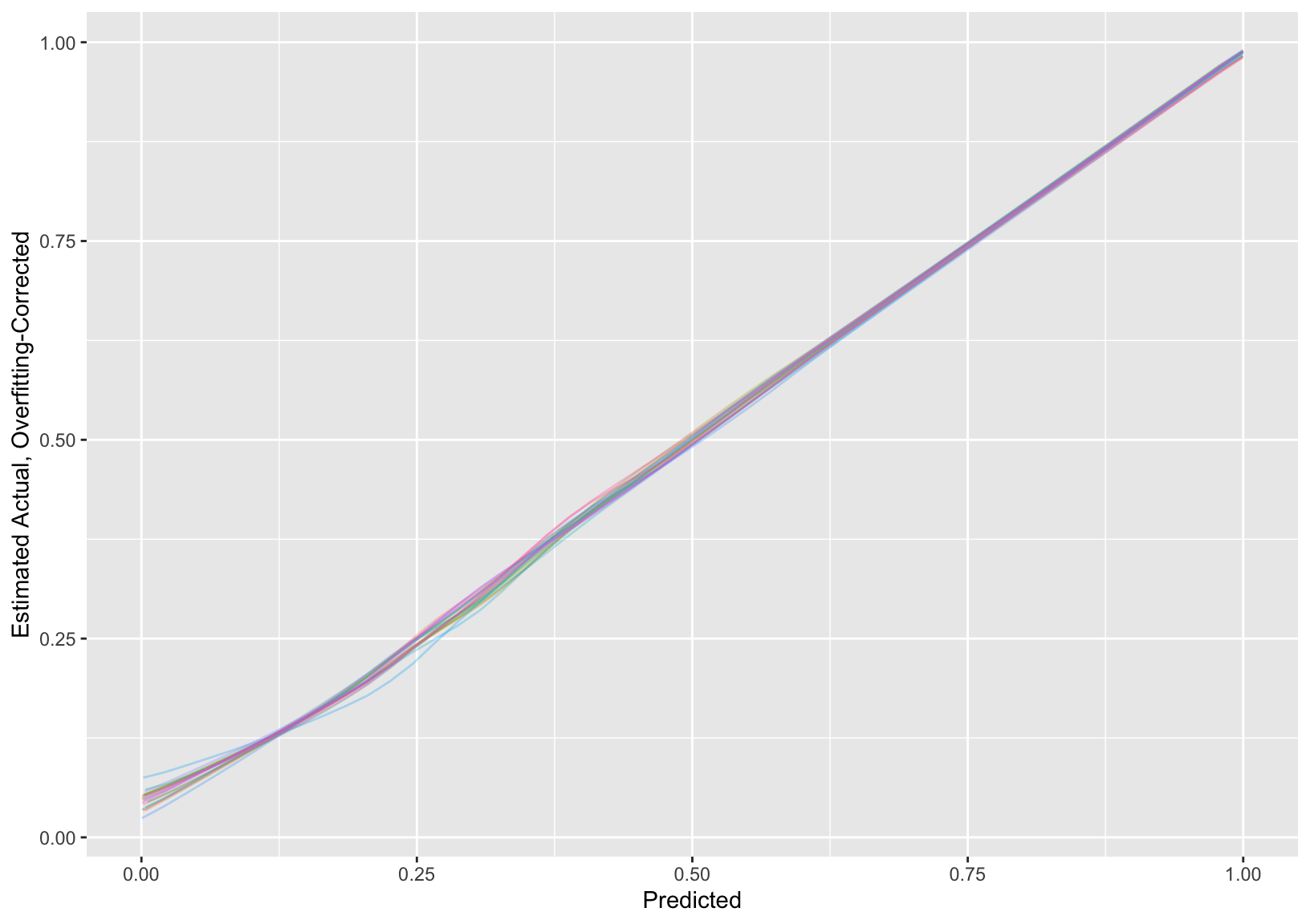
* Display the 20 bootstrap internal validations averaged over the multiple imputations.
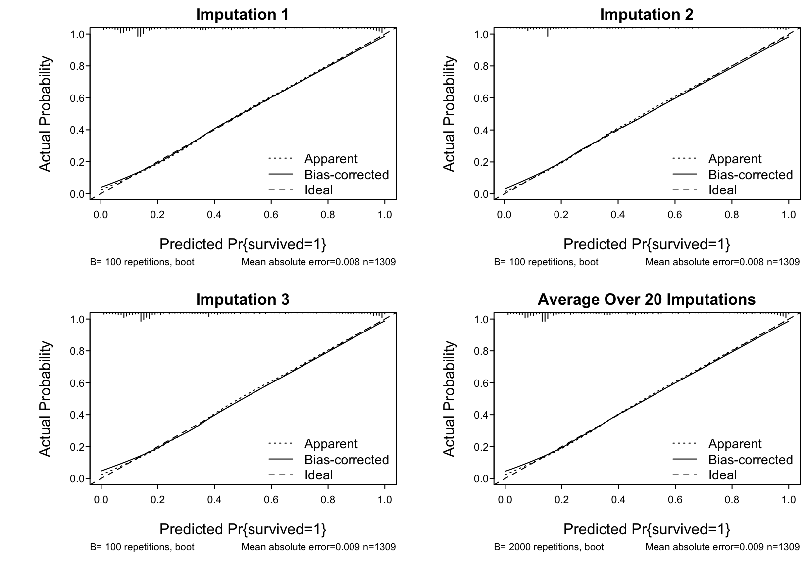
* Show the 20 individual calibration curves then the first 3 in more detail followed by the overall calibration estimate
```{r}
val <- processMI(f, 'validate')
print(val, digits=3)
```
```{r}
#| label: fig-titanic-calibrate
#| fig.cap: "Estimated calibration curves for the Titanic risk model, accounting for multiple imputation"
#| fig.width: 8.5
#| fig.height: 6
#| column: screen-inset-right
spar(mfrow=c(2,2), top=1, bot=2)
cal <- processMI(f, 'calibrate', nind=3)
# plot(cal) for full-size final calibration curve
```
Return to the stacked fit and compare it to the fit from single imputation
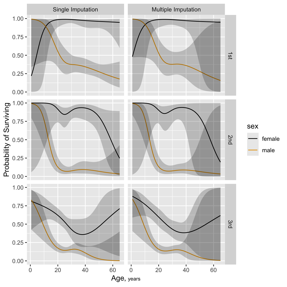
```{r namult, h=6, w=6, cap='Predicted probability of survival for males from fit using single conditional mean imputation again (top) and multiple random draw imputation (bottom). Both sets of predictions are for `sibsp`=0.',scap='Predicted Titanic survival using multiple imputation'}
#| label: fig-titanic-namult
p1 <- Predict(f.si,  age.i, pclass, sex, sibsp=0, fun=plogis)
p2 <- Predict(f.mi,  age,   pclass, sex, sibsp=0, fun=plogis)
p  <- rbind('Single Imputation'=p1, 'Multiple Imputation'=p2,
            rename=c(age.i='age'))
ggplot(p, groups='sex', ylab='Probability of Surviving')
```
## Summarizing the Fitted Model
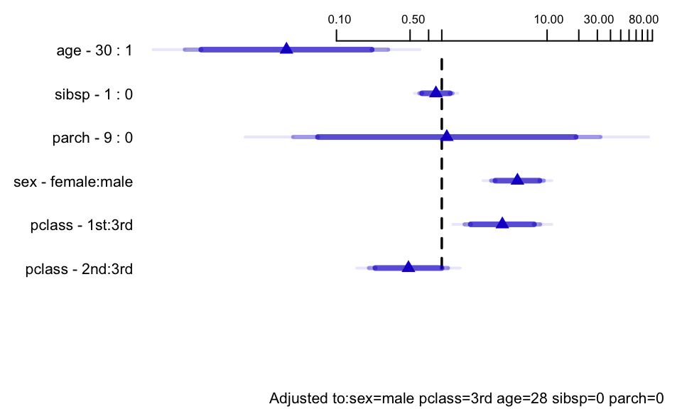
Show odds ratios for changes in predictor values `r ipacue()`
```{r ors, w=5, h=3, cap='Odds ratios for some predictor settings'}
#| label: fig-titanic-ors
spar(bot=1, top=0.5, ps=8)
# Get predicted values for certain types of passengers
s <- summary(f.mi, age=c(1,30), sibsp=0:1)
# override default ranges for 3 variables
plot(s, log=TRUE, main='')
```
```{r phat}
phat <- predict(f.mi,
                combos <-
         expand.grid(age=c(2,21,50),sex=levels(t3$sex),
                     pclass=levels(t3$pclass),
                     sibsp=0, parch=0), type='fitted')
# Can also use Predict(f.mi, age=c(2,21,50), sex, pclass,
#                      sibsp=0, fun=plogis)$yhat
options(digits=1)
data.frame(combos, phat)
options(digits=5)
```
We can also get predicted values by creating an R function that will `r ipacue()`
evaluate the model on demand, but that only works if there are no 3rd-order interactions.
```{r pred.logit,eval=FALSE}
pred.logit <- Function(f.mi)
# Note: if don't define sibsp to pred.logit, defaults to 0
plogis(pred.logit(age=c(2,21,50), sex='male', pclass='3rd'))
```
A nomogram could be used to obtain predicted values manually, but this `r ipacue()`
is not feasible when so many interaction terms are present.
## Bayesian Analysis
* Repeat the multiple imputation-based approach but using a `r ipacue()`
Bayesian binary logistic model
* Using default `blrm` function normal priors on regression
coefficients with zero mean and large SD making the priors almost flat
* `blrm` uses the `rcmdstan` and `rstan` packages that provides the full power of Stan to `R`
* Here we use `cmdstan` with `rcmdstan`
* `rmsb` has its own caching mechanism that efficiently stores the model fit object (and all its posterior draws) and reads it back from disk install of running it again, until one of the inputs change
* See [this](https://hbiostat.org/R/rmsb) for more about the `rmsb` package
* Could use smaller prior SDs to get penalized estimates
* Using 4 independent Markov chain Hamiltonion posterior sampling
procedures each with 1000 burn-in iterations that are discarded, and
1000 "real" iterations for a total of 4000 posterior sample draws
* Use the first 10 multiple imputations already developed
above (object `mi`), running the Bayesian procedure separately for 10 completed datasets
* Merely have to stack the posterior draws into one giant sample
to account for imputation and get correct posterior distribution
```{r blrm}
#| column: page-inset-right
# Use all available CPU cores less 1.  Each chain will be run on its
# own core.
require(rmsb)
options(mc.cores=parallel::detectCores() - 1, rmsb.backend='cmdstan')
cmdstanr::set_cmdstan_path(cmdstan.loc)
# cmdstan.loc is defined in ~/.Rprofile

# 10 Bayesian analyses took 3m on 11 cores
set.seed(21)
bt <- stackMI(survived ~ sex * pclass * rcs(age, 4) +
          rcs(age, 4) * (sibsp + parch),
          blrm, mi, data=t3, n.impute=10, refresh=25,
          file='bt.rds')
bt
```
* Note that fit indexes have HPD uncertainty intervals `r ipacue()`
* Everthing above accounts for imputation
* Look at diagnostics
::: {.callout-note collapse="true"}
### Separate Diagnostics for Each of 10 Imputed Datasets
```{r}
stanDx(bt)
```
:::
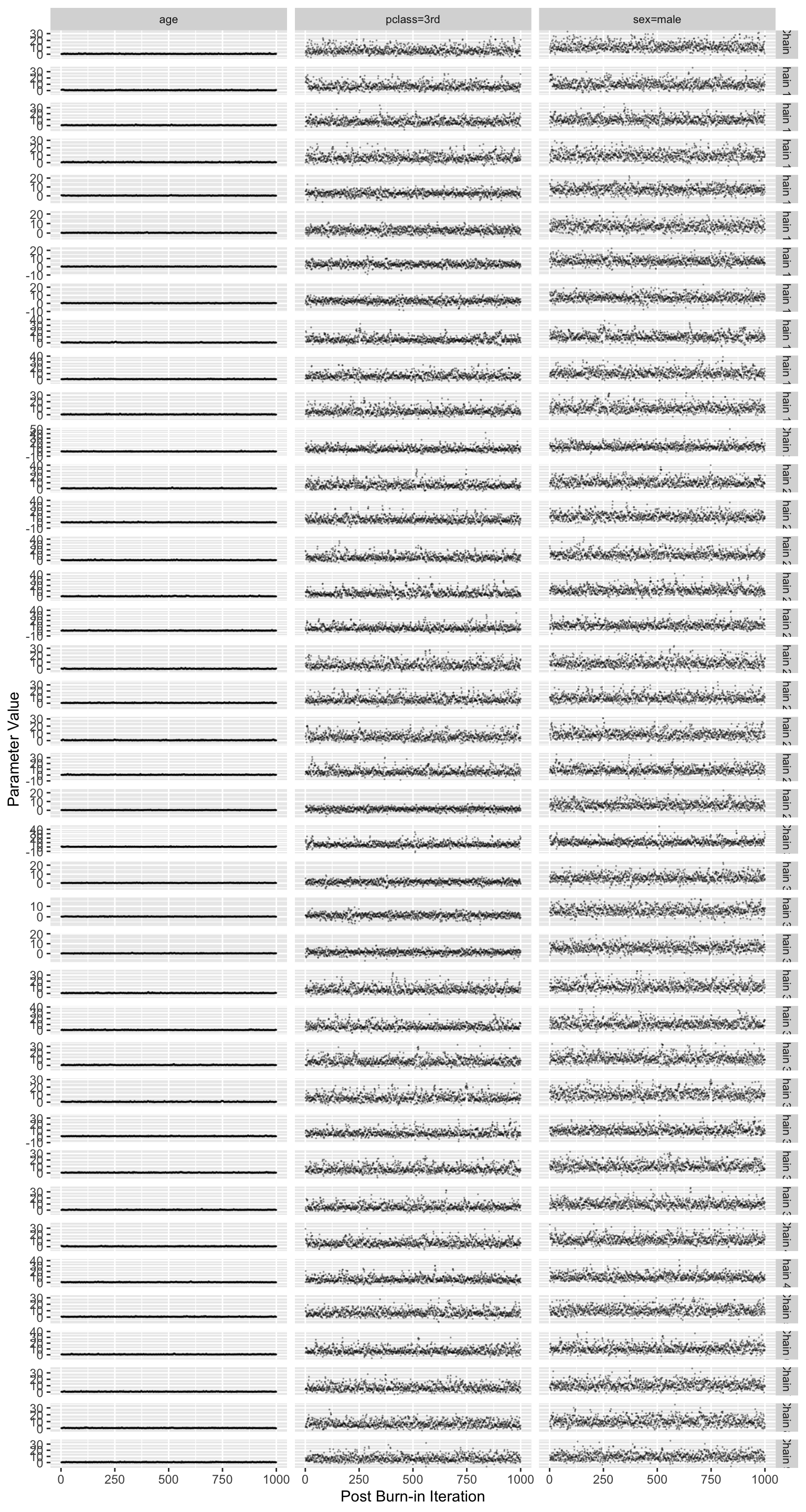
```{r blrmdx,w=8,h=15}
#| column: screen-right
# Look at convergence of only 2 parameters
stanDxplot(bt, c('sex=male', 'pclass=3rd', 'age'), rev=TRUE)
```
* Difficult to see but there are 40 traces (10 imputations `r ipacue()`
$\times$ 4 chains)
* Diagnostics look good; posterior samples can be trusted
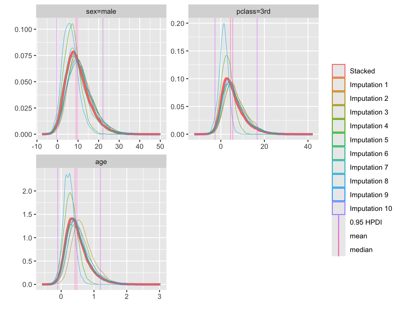
* Plot posterior densities for select parameters
* Also shows the 10 densities before stacking
```{r btdens,w=7,h=5.5}
plot(bt, c('sex=male', 'pclass=3rd', 'age'), nrow=2)
```
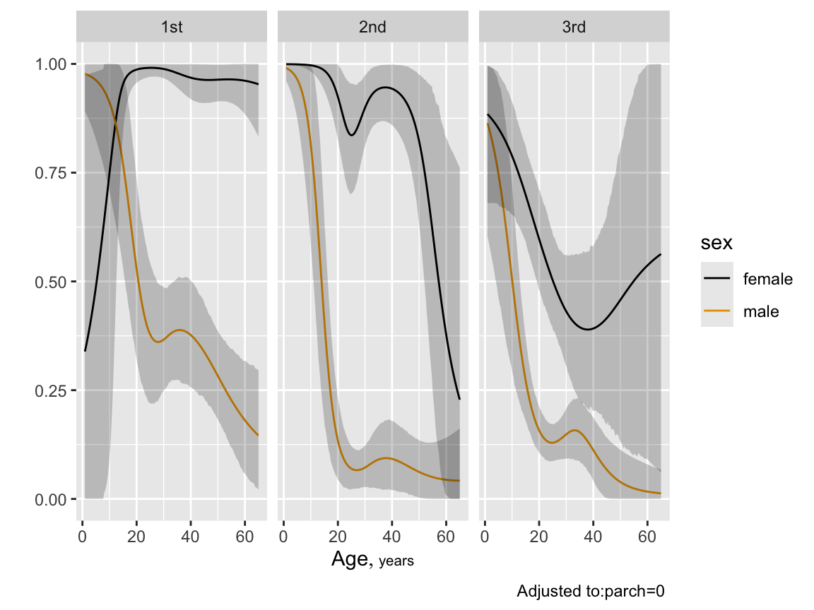
* Plot partial effect plots with 0.95 highest posterior density intervals `r ipacue()`
```{r btpe,w=6,h=4.5}
p <- Predict(bt, age, sex, pclass, sibsp=0, fun=plogis, funint=FALSE)
ggplot(p)
```
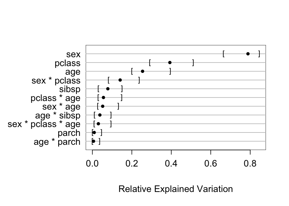
* Compute approximate measure of explained outcome variation for predictors `r ipacue()`
```{r bev,w=5.25,h=3.75}
plot(anova(bt))
```
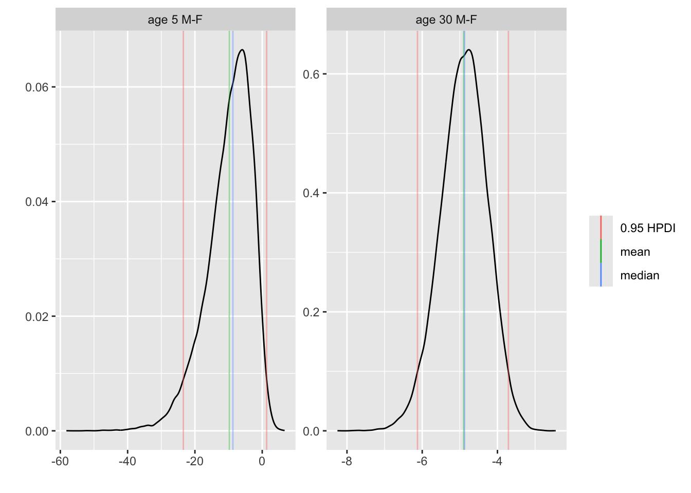
* Contrast second class males and females, both at 5 years and 30 `r ipacue()`
years of age, all other things being equal
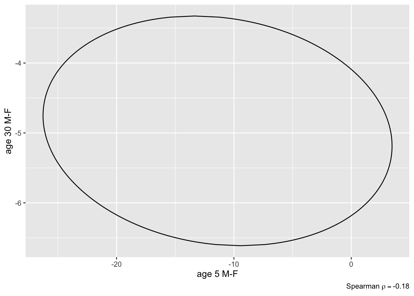
* Compute 0.95 HPD interval for the contrast and a joint
uncertainty region
* Compute P(both contrasts < 0), both < -2, and P(either one < 0)
```{r brcon}
k <- contrast(bt, list(sex='male',   age=c(5, 30), pclass='2nd'),
                  list(sex='female', age=c(5, 30), pclass='2nd'),
              cnames = c('age 5 M-F', 'age 30 M-F'))
k
plot(k)
```
```{r brcon2,fig.show='hold',out.width='3.5in'}
plot(k, bivar=TRUE)                        # assumes an ellipse
plot(k, bivar=TRUE, bivarmethod='kernel')  # doesn't
P <- PostF(k, pr=TRUE)
P(`age 5 M-F` < 0 & `age 30 M-F` < 0) # note backticks
P(`age 5 M-F` < -2 & `age 30 M-F` < -2)
P(`age 5 M-F` < 0 | `age 30 M-F` < 0)
```
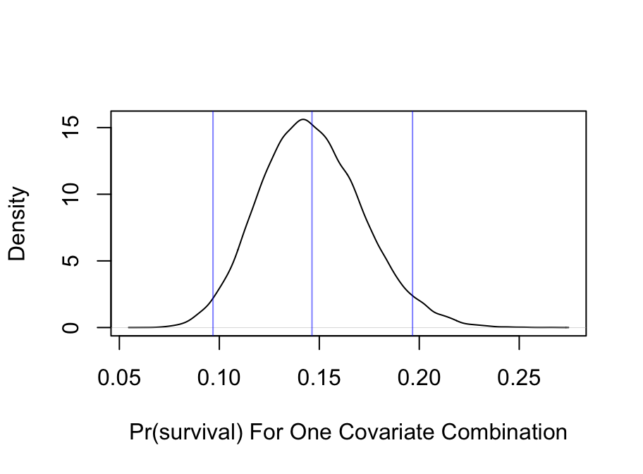
* Show posterior distribution of predicted survival probability for a 21 year old male in third class with `sibsp=0`
* `Predict` summarizes with a posterior mean (set `posterior.summary='median'` to use posterior median)
* Frequentist multiple imputation estimate was 0.1342
```{r}
#| fig.height: 3.5
#| fig.width: 4.75
pmean <- Predict(bt, age=21, sex='male', pclass='3rd', sibsp=0, parch=0,
                 fun=plogis, funint=FALSE)
pmean
p <- predict(bt,
             data.frame(age=21, sex='male', pclass='3rd', sibsp=0, parch=0),
             posterior.summary='all', fun=plogis, funint=FALSE)
plot(density(p), main='',
     xlab='Pr(survival) For One Covariate Combination')
abline(v=with(pmean, c(yhat, lower, upper)), col=alpha('blue', 0.5))
```
* Compute Pr(survival probability > 0.2) for this man
```{r}
mean(p > 0.2)
```
| Package | Purpose | Functions |
|-----|-----|-----|
| `Hmisc` | Miscellaneous functions | `summary,plsmo,naclus,llist,latex, summarize,Dotplot,describe` |
| `Hmisc` | Imputation | `transcan,impute,fit.mult.impute,aregImpute,stackMI` |
| `rms` | Modeling | `datadist,lrm,rcs` |
| | Accounting for imputation | `processMI, LRupdate` |
| | Model presentation | `plot,summary,nomogram,Function,anova` |
| | Estimation | `Predict,summary,contrast` |
| | Model validation | `validate,calibrate` |
| `rmsb` | Misc. Bayesian | `blrm`, `stanDx`,`stanDxplot`,`plot` |
| `rpart`^[Written by Atkinson and Therneau] | Recursive partitioning | `rpart` |
: `R` software used
```{r echo=FALSE}
saveCap('12')
```