```{r include=FALSE}
require(Hmisc)
options(qproject='rms', prType='html')
require(qreport)
getRs('qbookfun.r')
hookaddcap()
knitr::set_alias(w = 'fig.width', h = 'fig.height', cap = 'fig.cap', scap ='fig.scap')
```
# Semiparametric Ordinal Longitudinal Models
**MOST**: Markov Ordinal State Transition model
**Key references**
* @roh24bay; 2024 Statistics in Medicine tutorial
* [Navigating the landscape of hierarchical multi-component strategies: GPC, DOOR, and MOST](https://doi.org/10.48550/arXiv.2604.12662) by De Backer, Verbeeck, Lanius, Vandemeulebroecke, Evans, Hamasaki, Buyse, Harrell 2026
## Longitudinal Ordinal Models as Unifying Concepts
This material in this section is taken from [hbiostat.org/talks/rcteff.html](https://hbiostat.org/talks/rcteff.html).
See also [hbiostat.org/proj/covid19/ordmarkov.html](http://hbiostat.org/proj/covid19/ordmarkov.html) and [hbiostat.org/endpoint](https://hbiostat.org/endpoint) and [Ordinal state transition models as a unifying risk prediction framework](https://www.fharrell.com/talk/icsa).
### General Outcome Attributes
* Timing and severity of outcomes
* Handle
+ terminal events (death)
+ non-terminal events (MI, stroke)
+ recurrent events (hospitalization)
* Break the ties; the more levels of Y the better: [fharrell.com/post/ordinal-info](https://fharrell.com/post/ordinal-info)
+ Maximum power when there is only one patient at each level (continuous Y)
### What is a Fundamental Outcome Assessment?
* In a given week or day what is the severity of the worst thing that happened to the patient?
* Expert clinician consensus of outcome ranks
* Spacing of outcome categories irrelevant
* Avoids defining additive weights for multiple events on same week
* Events can be graded & can code common co-occurring events as worse event
* Can translate an ordinal longitudinal model to obtain a variety of estimates
+ time until a condition
+ expected time in state
* Bayesian partial proportional odds model can compute the probability that the treatment affects mortality differently than it affects nonfatal outcomes
* Model also elegantly handles partial information: at each day/week the ordinal Y can be left, right, or interval censored when a range of the scale was not measured
### Examples of Longitudinal Ordinal Outcomes
* 0=alive 1=dead
+ censored at 3w: 000
+ death at 2w: 01
+ longitudinal binary logistic model OR $\approx$ HR
* 0=at home 1=hospitalized 2=MI 3=dead
+ hospitalized at 3w, rehosp at 7w, MI at 8w \& stays in hosp, f/u ends at 10w: 0010001211
* 0-6 QOL excellent--poor, 7=MI 8=stroke 9=dead
+ QOL varies, not assessed in 3w but pt event free, stroke at 8w, death 9w: 12[0-6]334589
+ MI status unknown at 7w: 12[0-6]334[5-7]89^[Better: treat the outcome as being in one of two non-contiguous values {5,7} instead of [5-7] but no software is currently available for this]
+ Can make first 200 levels be a continuous response variable and the remaining values represent clinical event overrides
### Statistical Model
* Proportional odds ordinal logistic model with covariate adjustment
* Patient random effects (intercepts) handle intra-patient correlation
* Better fitting: Markov model
+ handles absorbing states, extremely high day-to-day correlations within subject
+ faster, flexible, uses standard software
+ state transition probabilities
+ after fit translate to unconditional state occupancy probabilities
+ use these to estimate expected time in a set of states (e.g.,
on ventilator or dead); restricted mean survival time without
assuming PH
* Extension of binary logistic model
* Generalization of Wilcoxon-Mann-Whitney Two-Sample Test
* No assumption about Y distribution for a given patient type
* Does not use the numeric Y codes
### Model Robustness {#sec-markov-robust}
* If $Y$ consists of different event types, model will not fit well unless non-PO is allowed for time
* Model has a high chance of finding the best treatment even if PO is assumed for treatment and it is strongly violated
* Probabiliity estimates for being in specific states may be inaccurate for some levels of $X$ if PO is falsely assumed for $X$
* State occupancy probabilities and expected time in states are relatively robust
* Uncertainties in $\hat{\beta}$ may be very inaccurate if correlation structure is badly misspecified
+ Frequentist: SEs too small and $\alpha$ inflated; Bayesian: posteriors too narrow, posterior probs miscalibrated
* Example: ORBITA <small>(Personal communication, Matthew Shun-Shin, Imperial College, London)</small>
+ Daily angina frequency with huge within-person variability
+ May lead a Markov model to think that prior states are irrelevant
+ $\rightarrow$ multiple observations on a subject have the same information as new subjects
+ $\rightarrow$ inflates apparent effective sample size
+ Need to incorporate each subject's latent angina tendencies to account for this
+ Most easily done with random intercepts
* Include random intercepts to protect against deflation of uncertainties in $\beta$
+ Serial correlation dominant structure $\rightarrow$ variance of random effects small and including them unnecessarily will not harm the analysis
+ Compound symmetry dominant structure $\rightarrow$ inclusion of lags in the model will not harm the analysis, and effects of lags may be small
+ Bayesian modeling handles random effects much more naturally
- Automatic marginalization over random effects when examining posterior draws for $\beta$
## Case Studies
* Random effects model for continuous Y: @sec-long-bayes-re
* Markov model for continuous Y: @sec-long-bayes-markov
* Multiple detailed case studies for discrete ordinal Y:
[hbiostat.org/proj/covid19](https://hbiostat.org/proj/covid19).
+ ORCHID: hydroxychloroquine for treatment of COVID-19 with
patient assessment on select days
+ VIOLET: vitamin D for serious respiratory illness with
assessment on 28 consecutive days
- Large power gain demonstrated over time to recovery or
ordinal status at a given day
- Loosely speaking serial assessments for each 5 day period
had the same statistical information as a new patient assessed once
+ ACTT-1: NIH-NIAID Remdesivir study
for treatment of COVID-19 with daily assessment while in hospital,
select days after that with interval censoring
- Assesses time-varying effect of remdesivir
- Handles death explicitly, unlike per-patient time to recovery
+ Other: Bayesian and frequentist power simulation, exploration
of unequal time gaps, etc.
## Case Study For 4-Level Ordinal Longitudinal Outcome
* VIOLET: randomized clinical trial of seriously ill adults in
ICUs to study the effectiveness of vitamin D vs. placebo
* Daily ordinal outcomes assessed for 28 days with very little missing data
* Original paper: [DOI:10.1056/NEJMoa1911124](https://www.nejm.org/doi/full/10.1056/NEJMoa1911124) focused on 1078 patients with confirmed baseline vitamin D deficiency
* Focus on 1352 of the original 1360 randomized patients
* Extensive re-analyses:
+ [hbiostat.org/proj/covid19/violet2.html](https://hbiostat.org/proj/covid19/violet2.html)
+ [hbiostat.org/proj/covid19/orchid.html](https://hbiostat.org/proj/covid19/orchid.html)
+ [hbiostat.org/R/Hmisc/markov/sim.html](https://hbiostat.org/R/Hmisc/markov/sim.html)
* Fitted a frequentist first-order Markov partial proportional
odds (PO) model to 1352 VIOLET patients using the `R` `VGAM`
package to simulate 250,000 patient longitudinal records with daily
assessments up to 28d: [hbiostat.org/data/repo/simlongord.html](http://hbiostat.org/data/repo/simlongord.html)
* Simulation inserted an odds ratio of 0.75 for `tx`=1 : `tx`=0 (log OR = -0.288)
* Case study uses the first 500 simulated patients
+ 13203 records
+ average of 26.4 records per patient out of a maximum of 28, due to deaths
+ full 250,00 and 500-patient datasets available at [hbiostat.org/data](https://hbiostat.org/data)
* 4-level outcomes:
+ patient at home
+ in hospital or other health facility
+ on ventilator or diagnosed with acute respiratory distress
syndrome (ARDS)
+ dead
* Death is an absorbing state
+ only possible _previous_ states are the first 3
+ at baseline no one was at home
+ a patient who dies has Dead as the status on their final
record, with no "deaths carried forward"
+ later we will carry deaths forward just to be able to look at
empirical state occupancy probabilities (SOPs) vs. model estimates
* Frequentist modeling using the `VGAM` package allows us to
use the unconstrained partial PO (PPO) model with regard to time,
but does not allow us to compute uncertainty intervals for derived
parameters (e.g., SOPs and mean time in states)
* Can use the bootstrap to obtain approximate confidence limits (as below)
* Bayesian analysis using the `rmsb` package provides exact uncertainty intervals for derived parameters but at present `rmsb` only implements the constrained PPO model when getting predicted values
* PPO for time allows mix of outcomes to change over time (which
occurred in the real data)
* Model specification:
+ For day $t$ let $Y(t)$ denote the ordinal outcome for a patient<br>
$\Pr(Y \geq y | X, Y(t-1)) = \text{expit}(\alpha_{y} + X\beta +
g(Y(t-1), t))$
+ $g$ contains regression coefficients for the previous state
$Y(t-1)$ effect, the absolute time $t$ effect, and any
$y$-dependency on the $t$ effect (non-PO for $t$)
+ Baseline covariates: `age`, `SOFA` score (a measure of organ
function), treatment (`tx`)
+ Time-dependent covariate: previous state (`yprev`, 3 levels)
+ Time trend: linear spline with knot at day 2 (handles exception at
day 1 when almost no one was sent home)
+ Changing mix of outcomes over time
- effect of time on transition ORs for different cutoffs of Y
- 2 time components (one slope change) $\times$ 3 Y cutoffs =
6 parameters related to `day`
* Reverse coding of Y so that higher levels are worse
### Descriptives
* all state transitions from one day to the next
* SOPs estimated by proportions (need to carry death forward)
```{r setdata}
require(rms)
require(data.table)
require(VGAM)
getHdata(simlongord500)
d <- simlongord500
setDT(d, key='id')
d[, y     := factor(y,     levels=rev(levels(y    )))]
d[, yprev := factor(yprev, levels=rev(levels(yprev)))]
setnames(d, 'time', 'day')
# Show descriptive statistics for baseline data
describe(d[day == 1, .(yprev, age, sofa, tx)], 'Baseline Variables')
# Check that death can only occur on the last day
d[, .(ddif=if(any(y == 'Dead')) min(day[y == 'Dead']) -
                                max(day) else NA_integer_),
          by=id][, table(ddif)]
```
```{r trans,h=7,w=7}
#| label: fig-markov-trans
#| fig-cap: "Transition proportions from data simulated from VIOLET"
require(ggplot2)
propsTrans(y ~ day + id, data=d, maxsize=4, arrow='->') +
    theme(axis.text.x=element_text(angle=90, hjust=1))
```
Show state occupancy proportions by creating a data table with death carried forward.
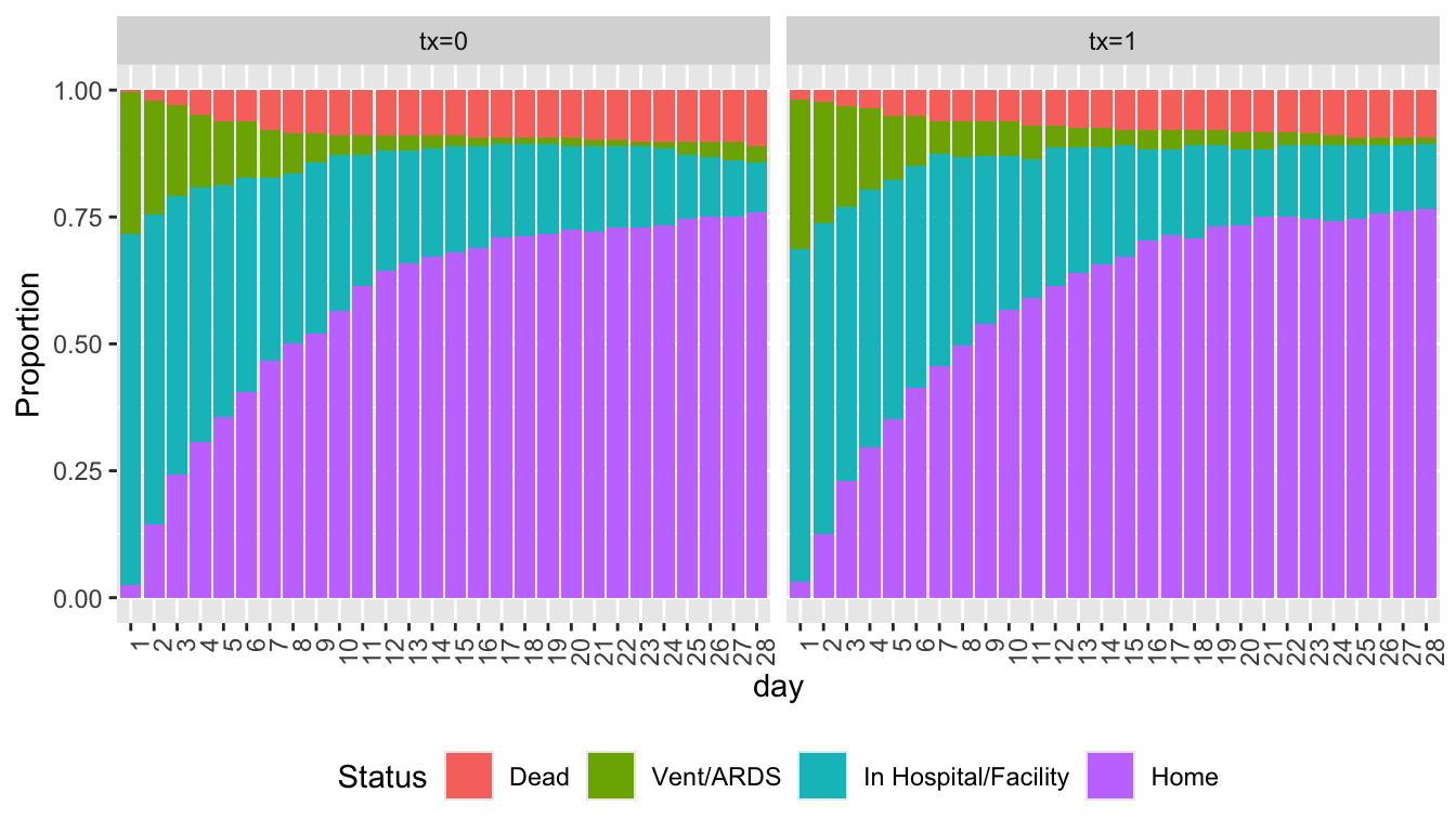
```{r soprops,w=7,h=4}
#| label: fig-markov-soprops
#| fig-cap: "State occupancy proportions from simulated VIOLET data with death carried forward"
w <- d[day < 28 & y == 'Dead', ]
w[, if(.N > 1) stop('Error: more than one death record'), by=id]
w <- w[, .(day = (day + 1) : 28, y = y, tx=tx), by=id]
u <- rbind(d, w, fill=TRUE)
setkey(u, id)
u[, Tx := paste0('tx=', tx)]
propsPO(y ~ day + Tx, data=u) +
  guides(fill=guide_legend(title='Status')) +
  theme(legend.position='bottom', axis.text.x=element_text(angle=90, hjust=1))
```
### Model Fitting
* Fit the PPO first-order Markov model without assuming PO for the time effect
* Also fit a model that has linear splines with more knots to add flexibility in how time and baseline covariates are transformed
* Disregard the terrible statistical practice of using asterisks to denote "significant" results
```{r ppofit}
f <- vglm(ordered(y) ~ yprev + lsp(day, 2) + age + sofa + tx,
          cumulative(reverse=TRUE, parallel=FALSE ~ lsp(day, 2)), data=d)
summary(f)
g <- vglm(ordered(y) ~ yprev + lsp(day, c(2, 4, 8, 15)) +
            lsp(age, c(35, 60, 75)) + lsp(sofa, c(2, 6, 10)) + tx,
          cumulative(reverse=TRUE, parallel=FALSE ~ lsp(day, c(2, 4, 8, 15))),
          data=d)
summary(g)
lrtest(g, f)
AIC(f); AIC(g)
```
We will use the simpler model, which has the better (smaller) AIC. Check the PO assumption on time by comparing the simpler model's AIC to the AIC from a fully PO model.
```{r testpo}
h <- vglm(ordered(y) ~ yprev + lsp(day, 2) + age + sofa + tx,
          cumulative(reverse=TRUE, parallel=TRUE), data=d)
lrtest(f, h)
AIC(f); AIC(h)
```
The model allowing for non-PO in time is better. Now show Wald tests on the parameters.
```{r }
wald <- function(f) {
  se <- sqrt(diag(vcov(f)))
  s <- round(cbind(beta=coef(f), SE=se, Z=coef(f) / se), 3)
  a <- c('>= in hospital/facility', '>= vent/ARDS', 'dead',
         'previous state in hospital/facility',
         'previous state vent/ARDS',
         'initial slope for day, >= hospital/facility',
         'initial slope for day, >= vent/ARDS',
         'initial slope for day, dead',
         'slope increment, >= hospital/facilty',
         'slope increment, >= vent/ARDS',
         'slope increament, dead',
         'baseline age linear effect',
         'baseline SOFA score linear effect',
         'treatment log OR')
  rownames(s) <- a
  s
}
wald(f)
```
We see evidence for a benefit of treatment. Compute the treatment transition OR and approximate 0.95 confidence interval.
```{r }
lor <- coef(f)['tx']
se  <- sqrt(vcov(f)['tx', 'tx'])
b   <- exp(lor + qnorm(0.975) * se * c(0, -1, 1))
names(b) <- c('OR', 'Lower', 'Upper')
round(b, 3)
```
The maximum likelihood estimate of the OR is somewhat at odds with the true OR of 0.75 on which the simulations were based.
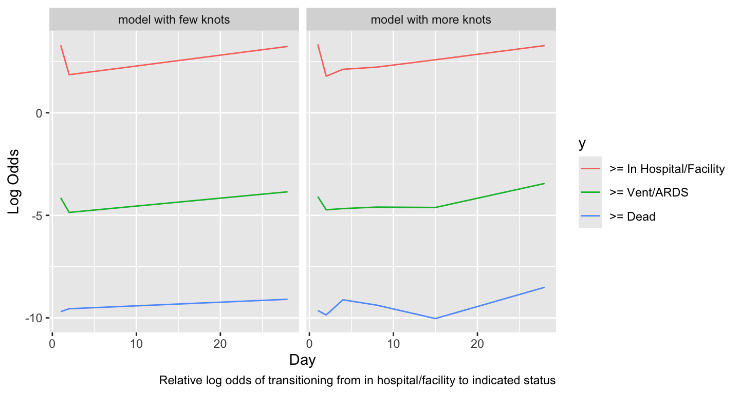
### Covariate Effects
* Most interesting covariate effect is effect of time since randomization
```{r timeeff,w=7.5,h=4}
#| label: fig-markov-timeeff
#| fig-cap: "Estimated time trends in relative log odds of transitions. Variables not shown are set to median/mode and `tx=0`."
#| fig-scap: "Estimated time trends in relative log transition odds"
w <- d[day == 1]
dat <- expand.grid(yprev = 'In Hospital/Facility', age=median(w$age),
                   sofa=median(w$sofa), tx=0, day=1:28)
ltrans <- function(fit, mod) {
  p <- predict(fit, dat)
  u <- data.frame(day=as.vector(row(p)), y=as.vector(col(p)), logit=as.vector(p))
  u$y   <- factor(u$y, 1:3, paste('>=', levels(d$y)[-1]))
  u$mod <- mod
  u
}
u <- rbind(ltrans(f, 'model with few knots'),
           ltrans(g, 'model with more knots'))
ggplot(u, aes(x=day, y=logit, color=y)) + geom_line() +
  facet_wrap(~ mod, ncol=2) +
  xlab('Day') + ylab('Log Odds') +
  labs(caption='Relative log odds of transitioning from in hospital/facility to indicated status')
```
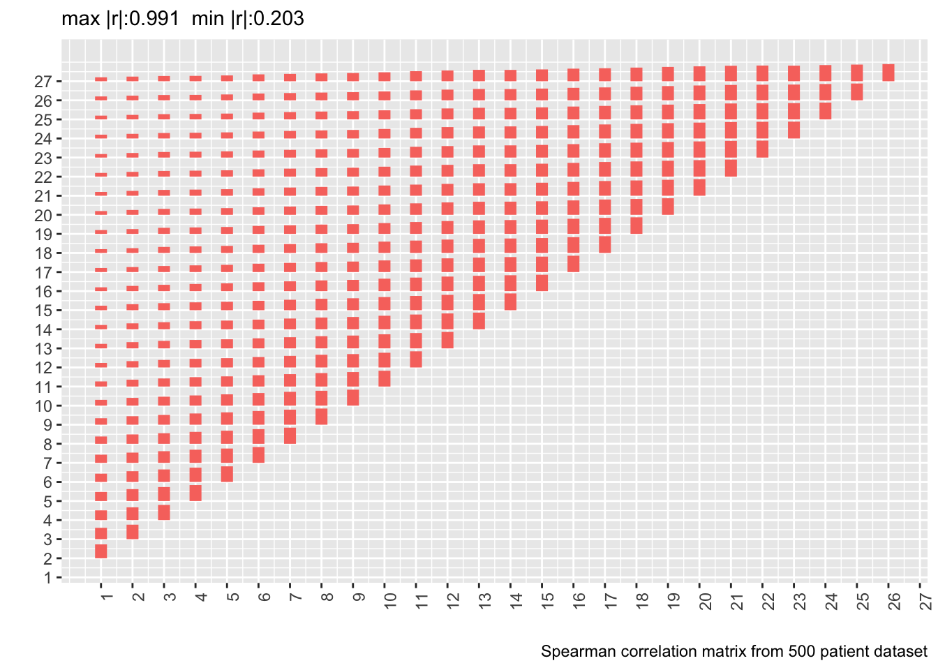
### Correlation Structure
* The data were simulated under a first-order Markov process so it doesn't make sense to check correlation pattern assumptions for our model
* When the simulated data were created, the within-patient correlation pattern was checked against the pattern from the fitted model by simulating a large trial from the model fit and comparing correlations in the simulated data to those in the real data
* It showed excellent agreement
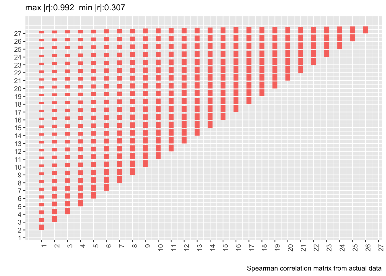
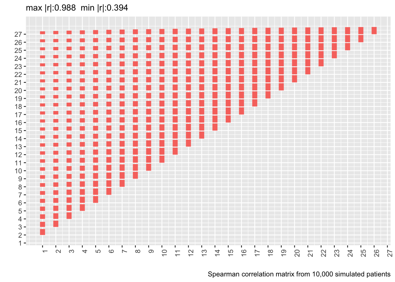
* Let's compute the Spearman $\rho$ correlation matrix on the 500 patient dataset and show the matrix from the real data next to it
* Delete day 28 from the new correlation matrix to conform with correlation matrix computed on real data
* Also show correlation matrix from 10,000 patient sample
* Heights of bars are proportional to Spearman $\rho$
```{r corm,fig.show='asis'}
# Tall and thin -> short and wide data table
w <- dcast(d[, .(id, day, y=as.numeric(y))],
           id ~ day, value.var='y')
r <- cor(as.matrix(w[, -1]), use='pairwise.complete.obs',
         method='spearman')[-28, -28]
p <- plotCorrM(r, xangle=90)
p[[1]] + theme(legend.position='none') +
  labs(caption='Spearman correlation matrix from 500 patient dataset')
vcorr <- readRDS('markov-vcorr.rds')
ra    <- vcorr$r.actual
plotCorrM(ra, xangle=90)[[1]] + theme(legend.position='none') +
  labs(caption='Spearman correlation matrix from actual data')
rc    <- vcorr$r.simulated
plotCorrM(rc, xangle=90)[[1]] + theme(legend.position='none') +
  labs(caption='Spearman correlation matrix from 10,000 simulated patients')
```
* Estimating the whole correlation matrix from 500 patients is noisy
* Compute the mean absolute difference between two correlation matrices (the first on 10,000 simulated patients assuming a first-order Markov process and the second from the real data)
* Compute means of mean absolute differences stratified by the day involved
```{r madr}
ad <- abs(rc[-28, -28] - ra)
round(apply(ad, 1, mean), 2)
```
Actual and simulated with-patient correlations agree well except when day 1 is involved.
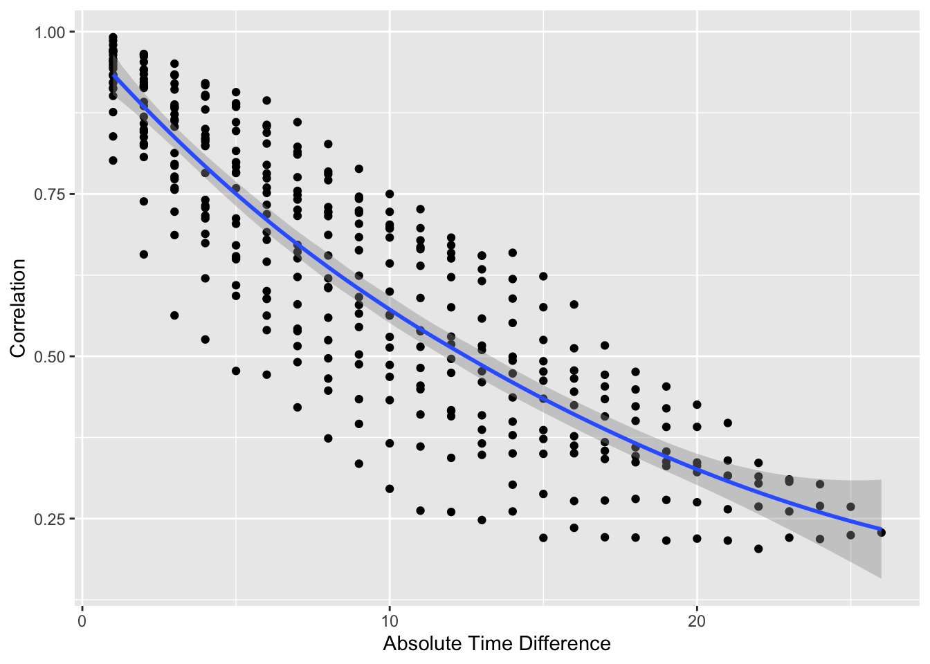
```{r vario}
#| label: fig-markov-vario
#| fig-cap: "Variogram-like graph for checking intra-patient correlation structure. $x$-axis shows the number of days between two measurements."
#| fig-scap: "Variogram-like graph"
p[[2]]
```
* Usual serial correlation declining pattern; outcome status values become less correlated within patient as time gap increases
* Also see non-isotropic pattern: correlations depend also on absolute time, not just gap
#### Formal Goodness of Fit Assessments for Correlation Structure
* Data simulation model $\rightarrow$ we already know that the first order Markov process has to fit
* Do two formal assessments to demonstrate how this can be done in general. Both make the correlation structure more versatile.
+ Add patient-specific intercepts to see if a compound symmetry structure adds anything to the first-order Markov structure
+ Add a dependency on state before last in addition to our model's dependency on the last state to see if a second-order Markov process fits better
**Add Random Effects**
* Bayesian models handle random effects more naturally than frequentist models $\rightarrow$ use a Bayesian partial PO first-order Markov model (`R` `rmsb` package)
* Use `cmdstan` software in place of the default of `rstan`
```{r bayesre}
require(rmsb)
cmdstanr::set_cmdstan_path(cmdstan.loc)   # cmdstan.loc is defined in ~/.Rprofile
options(prType='html')
# Use all but one core
options(mc.cores = parallel::detectCores() - 1, rmsb.backend='cmdstan')
seed <- 2   # The following took 15m using 4 cores
# Specify adapt_delta since the default of 0.8 resulted in divergent samples
b <- blrm(y ~ yprev + lsp(day, 2) + age + sofa + tx + cluster(id),
          ~ lsp(day, 2), data=d,
          sampling.args=list(adapt_delta = 0.95),
          file='markov-bppo.rds')
stanDx(b)
```
```{r bayesre2}
b
```
* Note that `blrm` parameterizes the partial PO parameters differently than `vglm`.
* Posterior median of the standard deviation of the random effects $\sigma_\gamma$ is 0.39
* This is fairly small on the logit scale in which most of the action takes place in $[-4, 4]$
* Random intercepts add an inconsequential improvement in the fit, justifying the Markov process' conditional (on prior state) independence assumption
* Another useful analysis would entail comparing the SD of the posterior distributions for the main parameters with and without inclusion of the random effects
**Second-order Markov Process**
* On follow-up days 2-28
* Frequentist partial PO model
```{r markov2}
# Derive time-before-last states (lag-1 `yprev`)
h <- d[, yprev2 := shift(yprev), by=id]
h <- h[day > 1, ]
# Fit first-order model ignoring day 1 so can compare to second-order
# We have to make time linear since no day 1 data
f1 <- vglm(ordered(y) ~ yprev + day + age + sofa + tx,
           cumulative(reverse=TRUE, parallel=FALSE ~ day), data=h)
f2 <- vglm(ordered(y) ~ yprev + yprev2 + day + age + sofa + tx,
           cumulative(reverse=TRUE, parallel=FALSE ~ day), data=h)
lrtest(f2, f1)
AIC(f1); AIC(f2)
```
* First-order model has better fit "for the money" by AIC
* Formal chunk test of second-order terms not impressive
### Computing Derived Quantities
From the fitted Markov state transition model, compute for one covariate setting and two treatments:
* state occupancy probabilities
* mean time in state
* differences between treatments in mean time in state
To specify covariate setting:
* most common initial state is `In Hospital/Facility` so use that
* within that category look at relationship between the two covariates
* they have no correlation so use the individual medians
```{r cov2}
istate <- 'In Hospital/Facility'
w <- d[day == 1 & yprev == istate, ]
w[, cor(age, sofa, method='spearman')]
x <- w[, lapply(.SD, median), .SDcols=Cs(age, sofa)]
adjto <- x[, paste0('age=', x[, age], '  sofa=', x[, sofa],
                    '  initial state=', istate)]
# Expand to cover both treatments and initial state
x <- cbind(tx=0:1, yprev=istate, x)
x
```
Compute all SOPs for each treatment. `soprobMarkovOrdm` is in `Hmisc`.
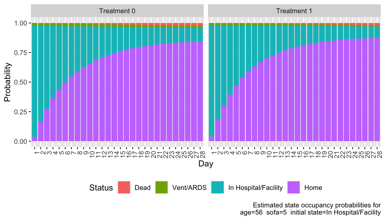
```{r sops,w=7,h=4}
#| label: fig-markov-sops
#| fig-cap: "State occupancy probabilities for each treatment"
S <- z <- NULL
for(Tx in 0:1) {
  s <- soprobMarkovOrdm(f, x[tx == Tx, ], times=1:28, ylevels=levels(d$y),
                        absorb='Dead', tvarname='day')
  S <- rbind(S, cbind(tx=Tx, s))
  u <- data.frame(day=as.vector(row(s)), y=as.vector(col(s)), p=as.vector(s))
  u$tx <- Tx
  z <- rbind(z, u)
}
z$y <- factor(z$y, 1:4, levels(d$y))
revo <- function(z) {
  z <- as.factor(z)
  factor(z, levels=rev(levels(as.factor(z))))
}
ggplot(z, aes(x=factor(day), y=p, fill=revo(y))) +
    facet_wrap(~ paste('Treatment', tx), nrow=1) + geom_col() +
    xlab('Day') + ylab('Probability') +
    guides(fill=guide_legend(title='Status')) +
    labs(caption=paste0('Estimated state occupancy probabilities for\n',
                        adjto)) +
    theme(legend.position='bottom',
          axis.text.x=element_text(angle=90, hjust=1))
```
Compute by treatment the mean time unwell (expected number of days not at home). Expected days in state is simply the sum over days of daily probabilities of being in that state.
```{r mtu}
mtu  <- tapply(1. - S[, 'Home'], S[, 'tx'], sum)
dmtu <- diff(mtu)
w    <- c(mtu, dmtu)
names(w) <- c('tx=0', 'tx=1', 'Days Difference')
w
```
We estimate that patients on treatment 1 have 1 less day unwell than those on treatment 0 for the given covariate settings.
Do a similar calculation for the expected number of days alive out of 28 days (similar to restricted mean survival time.
```{r mta}
mta <- tapply(1. - S[, 'Dead'], S[, 'tx'], sum)
w <- c(mta, diff(mta))
names(w) <- c('tx=0', 'tx=1', 'Days Difference')
w
```
### Bootstrap Confidence Interval for Difference in Mean Time Unwell
* Need to sample with replacement from _patients_, not records
+ code taken from `rms` package's `bootcov` function
+ sampling patients entails including some patients multiple times and omitting others
+ save all the record numbers, group them by patient ID, sample from these IDs, then use all the original records whose record numbers correspond to the sampled IDs
* Use the basic bootstrap to get 0.95 confidence intervals
* Speed up the model fit by having each bootstrap fit use as starting parameter estimates the values from the original data fit
```{r boot}
B         <- 500    # number of bootstrap resamples
recno     <- split(1 : nrow(d), d$id)
npt       <- length(recno)   # 500
startbeta <- coef(f)
seed      <- 3
if(file.exists('markov-boot.rds')) {
  z        <- readRDS('markov-boot.rds')
  betas    <- z$betas
  diffmean <- z$diffmean
} else {
  betas <- diffmean <- numeric(B)
  ylev  <- levels(d$y)
  for(i in 1 : B) {
    j <- unlist(recno[sample(npt, npt, replace=TRUE)])
    g <- vglm(ordered(y) ~ yprev + lsp(day, 2) + age + sofa + tx,
              cumulative(reverse=TRUE, parallel=FALSE ~ lsp(day, 2)),
              coefstart=startbeta, data=d[j, ])
    betas[i] <- coef(g)['tx']
    s0 <- soprobMarkovOrdm(g, x[tx == 0, ], times=1:28, ylevels=ylev,
                           absorb='Dead', tvarname='day')
    s1 <- soprobMarkovOrdm(g, x[tx == 1, ], times=1:28, ylevels=ylev,
                           absorb='Dead', tvarname='day')
    # P(not at home) =  1 - P(home); sum these probs to get E[days]
    mtud <- sum(1. - s1[, 'Home']) - sum(1. - s0[, 'Home'])
    diffmean[i] <- mtud
  }
  saveRDS(list(betas=betas, diffmean=diffmean), 'markov-boot.rds', compress='xz')
}
```
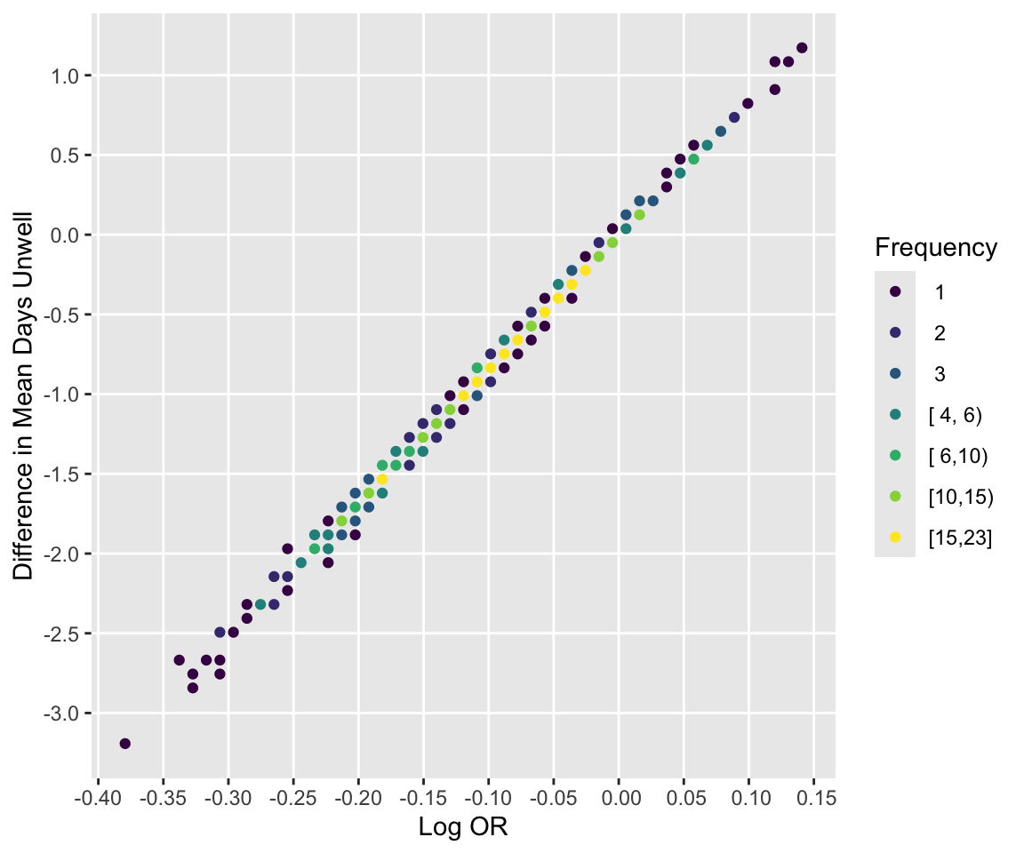
See how bootstrap treatment log ORs relate to differences in days unwell.
```{r compare,h=5,w=6}
#| label: fig-markov-compare
#| fig-cap: "Relationship between bootstrap log ORs and differences in mean days unwell"
ggfreqScatter(betas, diffmean,
              xlab='Log OR', ylab='Difference in Mean Days Unwell')
```
Compute basic bootstrap 0.95 confidence interval for OR and differences in mean time
```{r bootci}
# bootBCa is in the rms package and uses the boot package
clb <- exp(bootBCa(coef(f)['tx'], betas, seed=seed, n=npt, type='basic'))
clm <- bootBCa(dmtu, diffmean, seed=seed, n=npt, type='basic')
a   <- round(c(clb, clm), 3)[c(1,3,2,4)]
data.frame(Quantity=c('OR', 'Difference in mean days unwell'),
            Lower=a[1:2], Upper=a[3:4])
```
### Notes on Inference
* Differences between treatments in mean time in state(s) is zero if and only if the treatment OR=1
+ note agreement in bootstrap estimates
+ will not necessarily be true if PO is relaxed for treatment
+ inference about _any_ treatment effect is the same for all covariate settings that do not interact with treatment
+ $\rightarrow p$-values are the same for the two metrics, and Bayesian posterior probabilities are also identical
* Bayesian posterior probabilities for mean time in state $> \epsilon$, for $\epsilon > 0$, will vary with covariate settings (sicker patients at baseline have more room to move)
```{r echo=FALSE}
saveCap('22')
```