Without Risk Factor
|
With Risk Factor
|
|||
|---|---|---|---|---|
| Probability | Odds | Odds | Probability | |
| 0.20 | 0.25 | 0.5 | 0.333 | |
| 0.50 | 1.00 | 2.0 | 0.667 | |
| 0.80 | 4.00 | 8.0 | 0.889 | |
| 0.90 | 9.00 | 18.0 | 0.947 | |
| 0.98 | 49.00 | 98.0 | 0.990 | |
10 Binary Logistic Regression
A
- \(Y=0, 1\)
- Time of event not important
- In \(C(Y|X)\) \(C\) is \(\Pr(Y=1)\)
- \(g(u)\) is \(\frac{1}{1+e^{-u}} = \text{expit}(u)\)
10.1 Model
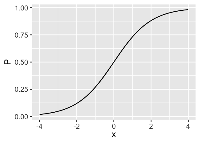
\[ \Pr(Y=1|X) = [1+\exp(-X\beta)]^{-1} \]
\[ P = [1+\exp(-x)]^{-1} = \text{expit}(x) \]
B
- \(O = \frac{P}{1-P}\)
- \(P = \frac{O}{1+O}\)
- \(X\beta = \log\frac{P}{1-P} = \text{logit}(P)\)
- \(e^{X\beta} = O\)
10.1.1 Model Assumptions and Interpretation of Parameters
C
- Increase \(X_{j}\) by \(d\) \(\rightarrow\) increase odds \(Y=1\) by \(\exp(\beta_{j}d)\), increase log odds by \(\beta_{j}d\).
- If there is only one predictor \(X\) and that predictor is binary, the model can be written
- One continuous predictor: \[ \text{logit}(Y=1|X) = \beta_{0}+\beta_{1} X, \]
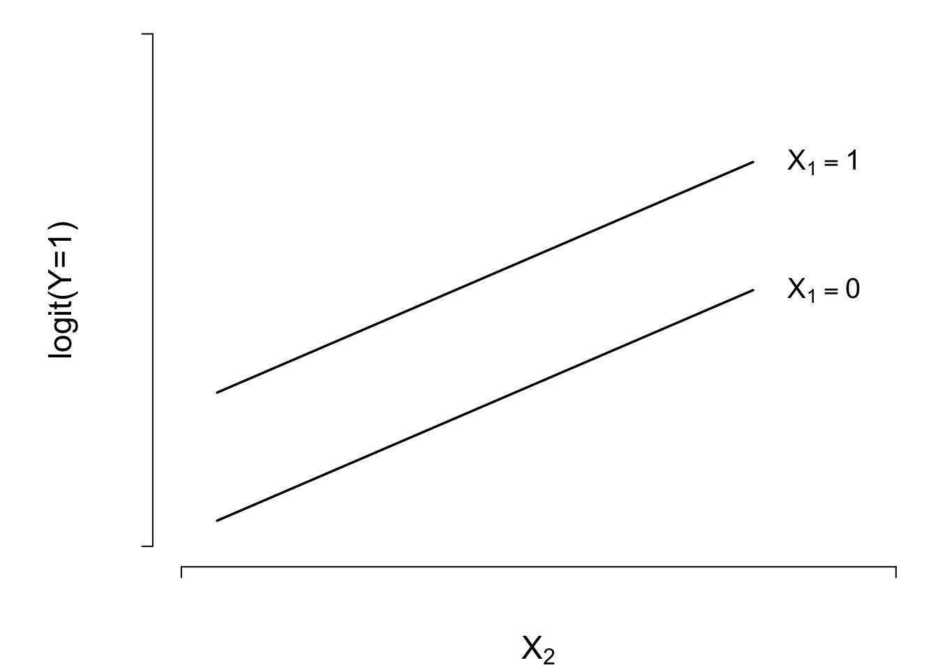
- Two treatments (indicated by \(X_{1}=0\) or \(1\)) and one continuous covariable (\(X_{2}\)). \[ \text{logit}(Y=1|X) = \beta_{0}+\beta_{1}X_{1}+\beta_{2}X_{2} , \]
10.1.2 Odds Ratio, Risk Ratio, and Risk Difference
D
- Odds ratio capable of being constant
- Ex: risk factor doubles odds of disease
Code
spar(bty='l')
plot(0, 0, type="n", xlab="Risk for Subject Without Risk Factor",
     ylab="Increase in Risk",
     xlim=c(0,1), ylim=c(0,.6))
i <- 0
or <- c(1.1,1.25,1.5,1.75,2,3,4,5,10)
for(h in or) {
  i <- i + 1
  p <- seq(.0001, .9999, length=200)
  logit <- log(p/(1 - p))  # same as qlogis(p)
  logit <- logit + log(h)  # modify by odds ratio
  p2 <- 1/(1 + exp(-logit))# same as plogis(logit)
  d <- p2 - p
  lines(p, d, lty=i)
  maxd <- max(d)
  smax <- p[d==maxd]
  text(smax, maxd + .02, format(h), cex=.6)
}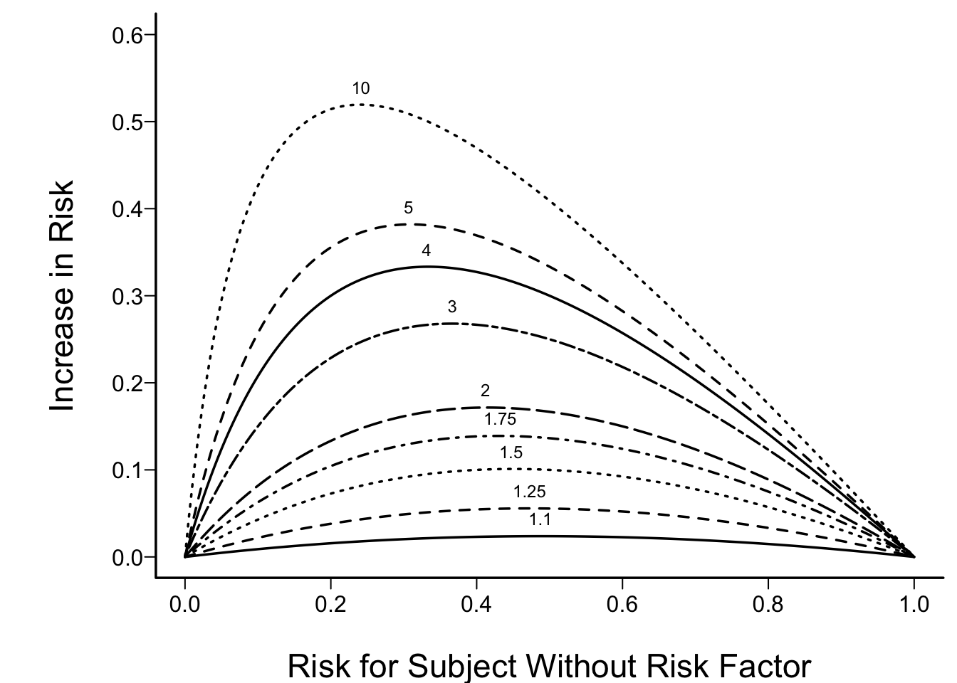
Let \(X_{1}\) be a binary risk factor and let
\(A=\{X_{2},\ldots,X_{p}\}\) be the other factors. Then the estimate of \(\Pr(Y=1|X_{1}=1, A) -\) \(\Pr(Y=1|X_{1}=0, A)\) is
E
where \(R=\Pr(Y=1|X_{1}=0, A)\).
- Risk ratio is \(\frac{1+e^{-X_{2}\beta}}{1+e^{-X_{1}\beta}}\)
- Does not simplify like odds ratio, which is \(\frac{e^{X_{1}\beta}}{e^{X_{2}\beta}} = e^{(X_{1}-X_{2})\beta}\)
10.1.3 Detailed Example
| Age: Females | 37 | 39 | 39 | 42 | 47 | 48 | 48 | 52 | 53 | 55 | 56 | 57 | 58 | 58 | 60 | 64 | 65 | 68 | 68 | 70 |
| Response: | 0 | 0 | 0 | 0 | 0 | 0 | 1 | 0 | 0 | 0 | 0 | 0 | 0 | 1 | 0 | 0 | 1 | 1 | 1 | 1 |
| Age: Males | 34 | 38 | 40 | 40 | 41 | 43 | 43 | 43 | 44 | 46 | 47 | 48 | 48 | 50 | 50 | 52 | 55 | 60 | 61 | 61 |
| Response: | 1 | 1 | 0 | 0 | 0 | 1 | 1 | 1 | 0 | 0 | 1 | 1 | 1 | 0 | 1 | 1 | 1 | 1 | 1 | 1 |
Code
require(rms)
options(prType='html')     # output format for certain rms functions
getHdata(sex.age.response)
d <- as.data.table(sex.age.response)  # so can do easy aggregation
dd <- datadist(d); options(datadist='dd')
f <- lrm(response ~ sex + age, data=d)
fasr <- f   # Save for later
p <- Predict(f, age=seq(34, 70, length=200), sex, fun=plogis)
# Function to bin a variable and represent bin by mean x within bin
mb <- function(x, ...) as.numeric(as.character(cut2(x, ..., levels.mean=TRUE)))
d[, ageg := mb(age, cuts=c(45, 55))]
props <- d[, .(prop = mean(response)), by=.(ageg, sex)]
ggplot(p, ylab='Pr(response)') +
  geom_point(data=d, aes(x=age, y=response, color=sex)) +
  geom_point(data=props, aes(x=ageg, y=prop, color=sex, shape=I(2)))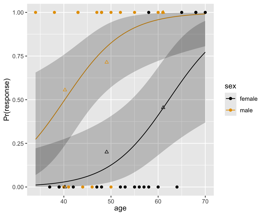
Code
ltx <- function(fit) {
  w <- latex(fit, inline=TRUE, columns=54,
             after='', digits=3,
             before='$$X\\hat{\\beta}=$$')
    rendHTML(w, html=FALSE)
  }
ltx(f)
\[X\hat{\beta}=\]
\[\begin{array}{l} -9.84\\ +3.49[\mathrm{male}] +0.158\:\mathrm{age} \end{array}\]
                 sex        response
                 Frequency
                 Row Pct      0        1    Total     Odds/Log

                 F           14        6       20    6/14=.429
                          70.00    30.00                 -.847

                 M            6       14       20    14/6=2.33
                          30.00    70.00                  .847

                 Total       20       20       40

                M:F odds ratio = (14/6)/(6/14) = 5.44, log=1.695
F
| Statistic | DF | Value | Prob |
|---|---|---|---|
| Wald \(\chi^2\) | 1 | 6.400 | 0.011 |
| Likelihood Ratio \(\chi^2\) | 1 | 6.583 | 0.010 |
| Parameter | Estimate | Std Err | Wald \(\chi^{2}\) | P |
|---|---|---|---|---|
| \(\beta_{0}\) | -0.847 | 0.488 | 3.015 | |
| \(\beta_{1}\) | 1.695 | 0.690 | 6.030 | 0.014 |
| Log likelihood (\(\beta_{1}=0\)) | -27.727 |
| Log likelihood (max) | -24.435 |
| LR \(\chi^{2} (H_{0}:\beta_{1}=0)\) -2(-27.727- -24.435) = 6.584 |
Next, consider the relationship between age and response, ignoring sex.
                 age        response
                 Frequency
                 Row Pct      0        1    Total     Odds/Log

                 <45          8        5       13     5/8=.625
                           61.5     38.4                  -.47

                 45-54        6        6       12        6/6=1
                           50.0     50.0                     0

                 55+          6        9       15      9/6=1.5
                           40.0     60.0                  .405

                 Total       20       20       40

                55+ : <45 odds ratio = (9/6)/(5/8) = 2.4, log=.875
G
| Parameter | Estimate | Std Err | Wald \(\chi^{2}\) | P |
|---|---|---|---|---|
| \(\beta_{0}\) | -2.734 | 1.838 | 2.213 | |
| \(\beta_{1}\) | 0.054 | 0.036 | 2.276 | 0.131 |
The estimate of \(\beta_{1}\) is in rough agreement with that obtained from the frequency table. The 55+:<45 log odds ratio is .875, and since the respective mean ages in the 55+ and <45 age groups are 61.1 and 40.2, an estimate of the log odds ratio increase per year is .875/(61.1 - 40.2)=.875/20.9=.042.
H
The likelihood ratio test for \(H_{0}\): no association between age and response is obtained as follows:
| Log likelihood (\(\beta_{1}=0\)) | -27.727 |
| Log likelihood (max) | -26.511 |
| LR \(\chi^{2} (H_{0}:\beta_{1}=0)\) | -2(-27.727- -26.511) = 2.432 |
(Compare 2.432 with the Wald statistic 2.28.)
Next we consider the simultaneous association of age and sex with response.
I
                                 sex=F

                 age        response
                 Frequency
                 Row Pct      0        1    Total

                 <45          4        0        4
                          100.0      0.0

                 45-54        4        1        5
                           80.0     20.0

                 55+          6        5       11
                           54.6     45.4

                 Total       14        6       20
J
                                 sex=M

                 age        response
                 Frequency
                 Row Pct      0        1    Total

                 <45          4        5        9
                           44.4     55.6

                 45-54        2        5        7
                           28.6     71.4

                 55+          0        4        4
                            0.0    100.0

                 Total        6       14       20
K
A logistic model for relating sex and age simultaneously to response is given below.
| Parameter | Estimate | Std Err | Wald \(\chi^{2}\) | P |
|---|---|---|---|---|
| \(\beta_{0}\) | -9.843 | 3.676 | 7.171 | |
| \(\beta_{1}\) (sex) | 3.490 | 1.199 | 8.469 | 0.004 |
| \(\beta_{2}\) (age) | 0.158 | 0.062 | 6.576 | 0.010 |
Likelihood ratio tests are obtained from the information below.
| Log likelihood (\(\beta_{1}=0,\beta_{2}=0\)) | -27.727 |
| Log likelihood (max) | -19.458 |
| Log likelihood (\(\beta_{1}=0\)) | -26.511 |
| Log likelihood (\(\beta_{2}=0\)) | -24.435 |
| LR \(\chi^{2}\) (\(H_{0}:\beta_{1}=\beta_{2}=0\)) | -2(-27.727- -19.458)= 16.538 |
| LR \(\chi^{2}\) (\(H_{0}:\beta_{1}=0\)) sex\(|\)age | -2(-26.511- -19.458) = 14.106 |
| LR \(\chi^{2}\) (\(H_{0}:\beta_{2}=0\)) age\(|\)sex | -2(-24.435- -19.458) = 9.954 |
The 14.1 should be compared with the Wald statistic of 8.47, and 9.954 should be compared with 6.58. Likelihood ratio tests may be obtained automatically starting in rms version 6.7-0, as follows.
L
Code
f <- update(f, x=TRUE, y=TRUE)   # LR tests require raw data in fits
anova(f, test='LR')
Likelihood Ratio Statistics for response |
|||
| χ2 | d.f. | P | |
|---|---|---|---|
| sex | 14.11 | 1 | 0.0002 |
| age | 9.95 | 1 | 0.0016 |
| TOTAL | 16.54 | 2 | 0.0003 |
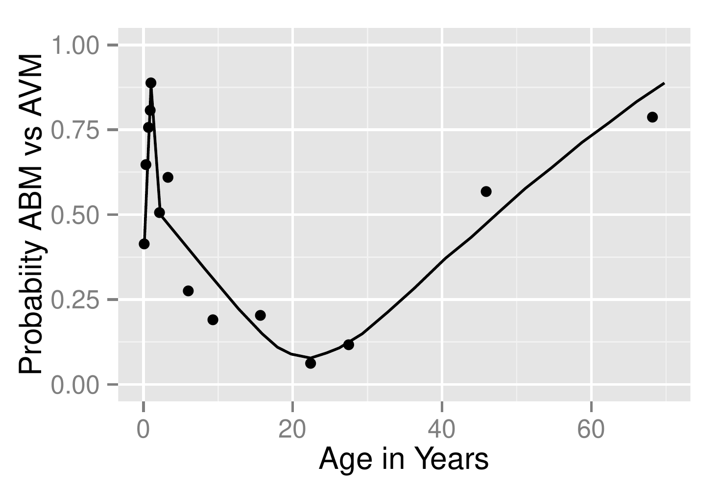
The fitted logistic model is plotted separately for females and males in Figure 10.3 .
The fitted model is
\[\Pr(\text{Response=1}|\text{sex,age}) = \text{expit}(-9.84+3.49\times \text{sex} +.158\times \text{age})\]
where as before sex=0 for females, 1 for males. For example, for a 40 year old female, the predicted logit is \(-9.84+.158(40) = -3.52\). The predicted probability of a response is \(\text{expit}(3.52)= .029\). For a 40 year old male, the predicted logit is \(-9.84 + 3.49+.158(40) = -.03\), with a probability of .492.
10.1.4 Design Formulations
M
- Can do ANOVA using \(k-1\) dummies for a \(k\)-level predictor
- Can get same \(\chi^2\) statistics as from a contingency table
- Can go farther: covariable adjustment
- Simultaneous comparison of multiple variables between two groups: Turn problem backwards to predict group from all the dependent variables
- This is more robust than a parametric multivariate test
- Propensity scores for adjusting for nonrandom treatment selection: Predict treatment from all baseline variables
- Adjusting for the predicted probability of getting a treatment adjusts adequately for confounding from all of the variables
- In a randomized study, using logistic model to adjust for covariables, even with perfect balance, will improve the treatment effect estimate
N
10.2 Estimation
10.2.1 Maximum Likelihood Estimates
Like binomial case but \(P\)s vary; \(\hat{\beta}\) computed by trial and error using an iterative maximization technique
10.2.2 Estimation of Odds Ratios and Probabilities
\[\hat{P}_{i} = \text{expit}(X_{i}\hat{\beta})\]
\[\text{expit}(X_{i}\hat{\beta}\pm zs)\]
10.2.3 Minimum Sample Size Requirement
- See this and this for detailed examples of power-based sample size calculations for the proportional odds model
O
Categorical Predictor Case
- Simplest case: no covariates, only an intercept
- Consider margin of error of 0.1 in estimating \(\theta = \Pr(Y=1)\) with 0.95 confidence
- Worst case: \(\theta = \frac{1}{2}\)
- Requires \(n=96\) observations1
- Single binary predictor with prevalence \(\frac{1}{2}\): need \(n=96\) for each value of \(X\)
- For margin of error of \(\pm 0.05, n=384\) is required (if true probabilities near 0.5 are possible); \(n=246\) required if true probabilities are only known not to be in \([0.2, 0.8]\).
1 The general formula for the sample size required to achieve a margin of error of \(\delta\) in estimating a true probability of \(\theta\) at the 0.95 confidence level is \(n = (\frac{1.96}{\delta})^{2} \times \theta(1 - \theta)\). Set \(\theta = \frac{1}{2}\) for the worst case.
Single Continuous Predictor
- Predictor \(X\) has a normal distribution with mean zero and standard deviation \(\sigma\), with true \(P = \text{expit}(X)\) so that the expected number of events is \(\frac{n}{2}\). Compute mean and 0.9 quantile of \(\max_{X \in [-1.5,1.5]} |P - \hat{P}|\) over 1000 simulations for varying \(n\) and \(\sigma\)2
PSee this for more about R coding for simulations of this type.
2 An average absolute error of 0.05 corresponds roughly to a 0.95 confidence interval margin of error of 0.1.
Code
require(rms)
require(ggplot2)

g <- function() {
set.seed(12)
sigmas  <- c(.5, .75, 1, 1.25, 1.5, 1.75, 2, 2.5, 3, 4)
ns      <- seq(25, 500, by=25)
nsim    <- 1000
xs      <- seq(-1.5, 1.5, length=200)
pactual <- plogis(xs)

dn     <- list(sigma=format(sigmas), n=format(ns), sim=NULL)
maxerr <- array(NA, c(length(sigmas), length(ns), nsim), dn)

i <- 0
for(s in sigmas) {
  i <- i + 1
  j <- 0
  for(n in ns) {
    j <- j + 1
    for(k in 1:nsim) {
      x <- rnorm(n, 0, s)
      P <- plogis(x)
      y <- ifelse(runif(n) <= P, 1, 0)
      beta <- lrm.fit(x, y)$coefficients
      phat <- plogis(beta[1] + beta[2] * xs)
      maxerr[i, j, k] <- max(abs(phat - pactual))
    }
  }
}
f  <- function(x) c(Mean=mean(x), Q90=unname(quantile(x, probs=0.9)))
apply(maxerr, 1:2, f)   # summarize over 3rd dimension (1000 simulations)
}

me    <- runifChanged(g)
# Function to create a variable holding value for ith dimension
slice <- function(a, i) {
  dn <- all.is.numeric(dimnames(a)[[i]], 'vector')   # all.is.numeric in Hmisc
  dn[as.vector(slice.index(a, i))]
}
u <- data.frame(maxerr = as.vector(me),
                stat   = slice(me, 1),
                sigma  = slice(me, 2),
                n      = slice(me, 3))
ggplot(u, aes(x=n, y=maxerr, color=factor(sigma))) + geom_line() +
  facet_wrap(~ stat) +
  ylab(expression(max(abs(hat(P) - P)))) +
  guides(color=guide_legend(title=expression(sigma))) +
  theme(legend.position='bottom')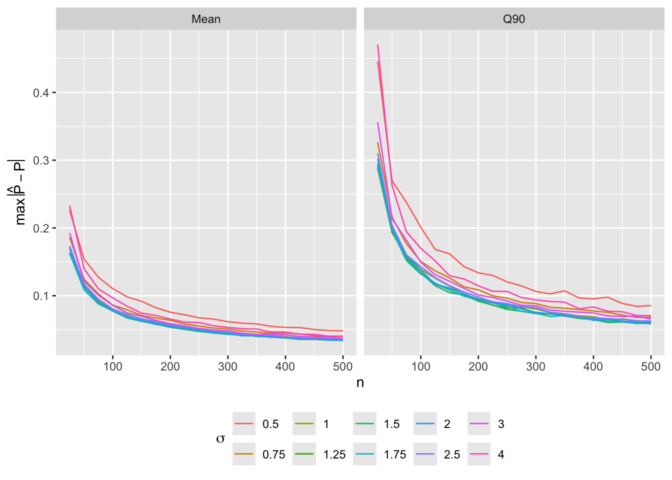
10.3 Test Statistics
Q
- Likelihood ratio test best
- Score test second best (score \(\chi^{2} \equiv\) Pearson \(\chi^2\))
- Wald test may misbehave but is quick
10.4 Residuals
Partial residuals (to check predictor transformations)
R
\[r_{ij} = \hat{\beta}_{j}X_{ij} + \frac{Y_{i} - \hat{P}_{i}}{\hat{P}_{i}(1-\hat{P}_{i})}\]
10.5 Assessment of Model Fit
S
\[\text{logit}(Y=1|X) = \beta_{0}+\beta_{1}X_{1}+\beta_{2}X_{2}\]
Code
getHdata(acath)
acath$sex <- factor(acath$sex, 0:1, c('male','female'))
dd <- datadist(acath); options(datadist='dd')
f <- lrm(sigdz ~ rcs(age, 4) * sex, data=acath)
kn <- specs(f)$how.modeled['age','Parameters']
kn <- setdiff(strsplit(kn, ' ')[[1]], '')
kn[length(kn)] <- paste('and', kn[length(kn)])
kn <- paste(kn, collapse=', ')
Code
d <- as.data.table(acath)
d[, ageg := mb(age, g=10)]   # bin into deciles of age
# Compute logit of proportion of disease in each decile and sex group
binned <- d[, .(logitprop = qlogis(mean(sigdz))), by=.(ageg, sex)]
# Estimate loess curves separately by sex
# Function to compute logit of loess nonparametric estimates for binary y
loel <- function(x, y, xlim) {
  j <- ! is.na(x + y)
  x <- x[j]; y <- y[j]
  z <- lowess(x, y, iter=0)
  i <- if(missing(xlim)) TRUE else z$x >= xlim[1] & z$x <= xlim[2]
  list(x=z$x[i], y=qlogis(z$y[i]))
}
loe <- d[, loel(age, sigdz, xlim=c(25, 78)), by=.(sex)]
ggplot(Predict(f, age, sex)) +
  geom_point(data=binned, aes(x=ageg, y=logitprop, color=sex, shape=I(2))) +
  geom_line(data=loe, aes(x=x, y=y, color=sex, linetype=I(2)))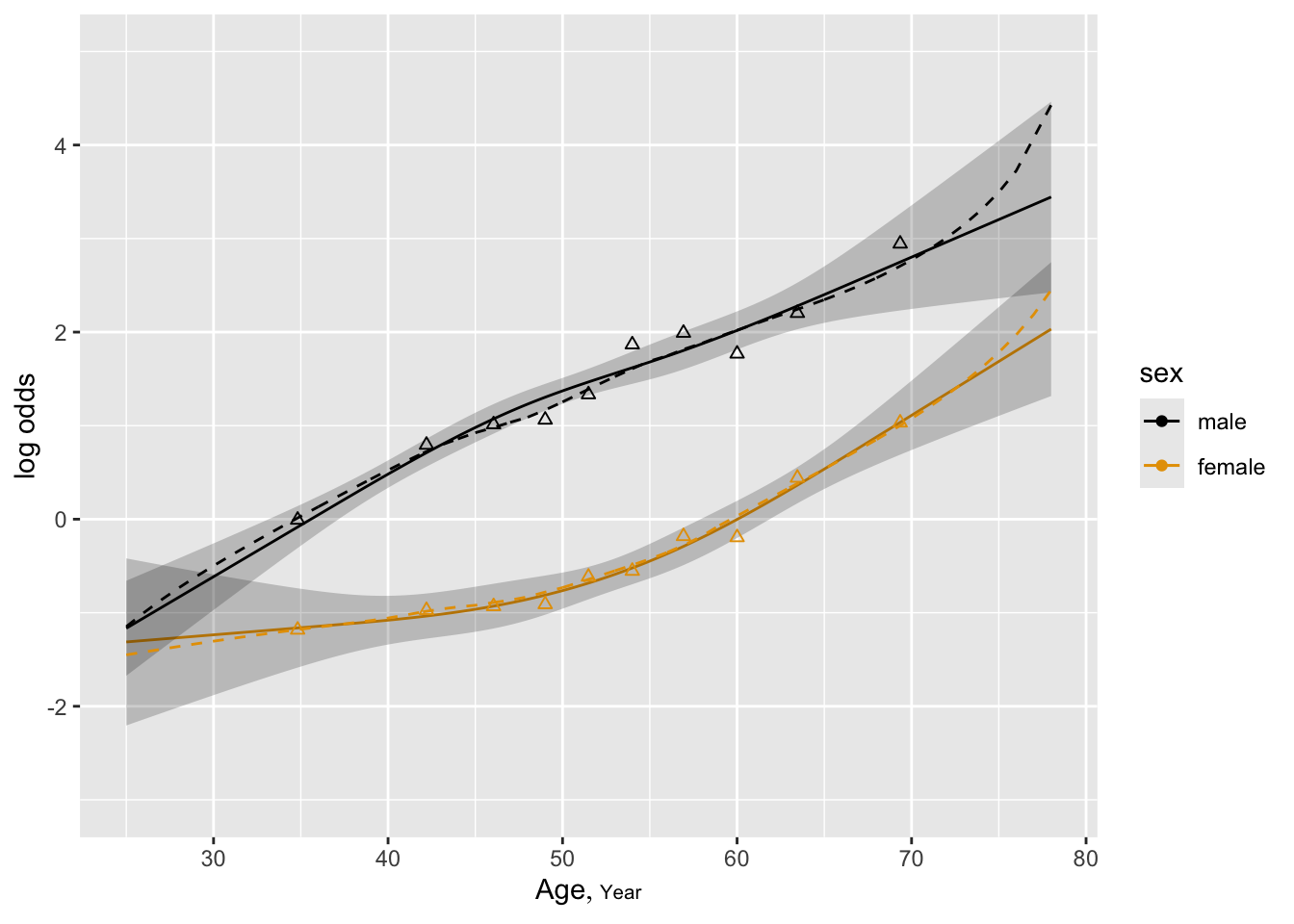
T
- Can verify by plotting stratified proportions
- \(\hat{P}\) = number of events divided by stratum size
- \(\hat{O} = \frac{\hat{P}}{1-\hat{P}}\)
- Plot \(\log \hat{O}\) (scale on which linearity is assumed)
- Stratified estimates are noisy
- 1 or 2 \(X\)s \(\rightarrow\) nonparametric smoother
- Use loess to compute logits of nonparametric estimates (
fun=qlogis) - General: restricted cubic spline expansion of one or more predictors
U
\[\begin{array}{ccc}
\text{logit}(Y=1|X) &=& \hat{\beta}_{0}+\hat{\beta}_{1}X_{1}+\hat{\beta}_{2}X_{2}+\hat{\beta}_{3}X_{2}'+\hat{\beta}_{4}X_{2}'' \nonumber \\
&=& \hat{\beta}_{0}+\hat{\beta}_{1}X_{1}+f(X_{2}) ,
\end{array}\]
\[\begin{array}{ccc}
\text{logit}(Y=1|X) &=& \beta_{0}+\beta_{1}X_{1}+\beta_{2}X_{2}+\beta_{3}X_{2}'+\beta_{4}X_{2}'' \nonumber \\
&& +\beta_{5}X_{1}X_{2}+\beta_{6}X_{1}X_{2}'+\beta_{7}X_{1}X_{2}''
\end{array}\]
V
Code
lr <- function(formula)
  {
    f <- lrm(formula, data=acath)
    stats <- f$stats[c('Model L.R.', 'd.f.')]
    cat('L.R. Chi-square:', round(stats[1],1),
        '  d.f.:', stats[2],'\n')
    f
  }
a <- lr(sigdz ~ sex + age)
L.R. Chi-square: 766 d.f.: 2 Code
b <- lr(sigdz ~ sex * age)L.R. Chi-square: 768.2 d.f.: 3 Code
c <- lr(sigdz ~ sex + rcs(age,4))L.R. Chi-square: 769.4 d.f.: 4 Code
d <- lr(sigdz ~ sex * rcs(age,4))L.R. Chi-square: 782.5 d.f.: 7 Code
lrtest(a, b)
Model 1: sigdz ~ sex + age
Model 2: sigdz ~ sex * age

L.R. Chisq       d.f.          P
 2.1964146  1.0000000  0.1383322
Code
lrtest(a, c)
Model 1: sigdz ~ sex + age
Model 2: sigdz ~ sex + rcs(age, 4)

L.R. Chisq       d.f.          P
 3.4502500  2.0000000  0.1781508
Code
lrtest(a, d)
Model 1: sigdz ~ sex + age
Model 2: sigdz ~ sex * rcs(age, 4)

  L.R. Chisq         d.f.            P
16.547036344  5.000000000  0.005444012
Code
lrtest(b, d)
Model 1: sigdz ~ sex * age
Model 2: sigdz ~ sex * rcs(age, 4)

  L.R. Chisq         d.f.            P
14.350621767  4.000000000  0.006256138
Code
lrtest(c, d)
Model 1: sigdz ~ sex + rcs(age, 4)
Model 2: sigdz ~ sex * rcs(age, 4)

  L.R. Chisq         d.f.            P
13.096786352 3.000000000 0.004431906 | Model / Hypothesis | Likelihood Ratio \(\chi^2\) | d.f. | \(P\) | Formula |
|---|---|---|---|---|
| a: sex, age (linear, no interaction) | 766.0 | 2 | ||
| b: sex, age, age \(\times\) sex | 768.2 | 3 | ||
| c: sex, spline in age | 769.4 | 4 | ||
| d: sex, spline in age, interaction | 782.5 | 7 | ||
| \(H_{0}:\) no age \(\times\) sex interaction given linearity | 2.2 | 1 | .14 | (\(b-a\)) |
| \(H_{0}:\) age linear \(|\) no interaction | 3.4 | 2 | .18 | (\(c-a\)) |
| \(H_{0}:\) age linear, no interaction | 16.6 | 5 | .005 | (\(d-a\)) |
| \(H_{0}:\) age linear, product form interaction | 14.4 | 4 | .006 | (\(d-b\)) |
| \(H_{0}:\) no interaction, allowing for nonlinearity in age | 13.1 | 3 | .004 | (\(d-c\)) |
Obtain all the fully adjusted likelihood ratio \(\chi^2\) tests automatically.
Code
f <- lrm(sigdz ~ sex * rcs(age,4), data=acath, x=TRUE, y=TRUE)
anova(f, test='LR')
Likelihood Ratio Statistics for sigdz |
|||
| χ2 | d.f. | P | |
|---|---|---|---|
| sex (Factor+Higher Order Factors) | 555.62 | 4 | <0.0001 |
| All Interactions | 13.10 | 3 | 0.0044 |
| age (Factor+Higher Order Factors) | 358.90 | 6 | <0.0001 |
| All Interactions | 13.10 | 3 | 0.0044 |
| Nonlinear (Factor+Higher Order Factors) | 14.35 | 4 | 0.0063 |
| sex × age (Factor+Higher Order Factors) | 13.10 | 3 | 0.0044 |
| Nonlinear | 9.67 | 2 | 0.0080 |
| Nonlinear Interaction : f(A,B) vs. AB | 9.67 | 2 | 0.0080 |
| TOTAL NONLINEAR | 14.35 | 4 | 0.0063 |
| TOTAL NONLINEAR + INTERACTION | 16.55 | 5 | 0.0054 |
| TOTAL | 782.54 | 7 | <0.0001 |
- Example of finding transform. of a single continuous predictor
- Duration of symptoms vs. odds of severe coronary disease
- Look at AIC to find best # knots for the money
| k | Model \(\chi^{2}\) | AIC |
|---|---|---|
| 0 | 99.23 | 97.23 |
| 3 | 112.69 | 108.69 |
| 4 | 121.30 | 115.30 |
| 5 | 123.51 | 115.51 |
| 6 | 124.41 | 114.41 |
Code
d  <- as.data.table(acath)[sigdz == 1]
dd <- datadist(d)
f <- lrm(tvdlm ~ rcs(cad.dur, 5), data=d)
d[, durg := mb(cad.dur, g=15)]   # bin into 15-tiles of age
# Compute logit of proportion of severe dz in each bin
binned <- d[, .(logitprop = qlogis(mean(tvdlm))), by=.(durg)]
loe <- d[, loel(cad.dur, tvdlm, xlim=c(0, 326))]
ggplot(Predict(f, cad.dur)) +
  geom_point(data=binned, aes(x=durg, y=logitprop, shape=I(2))) +
  geom_line(data=loe, aes(x=x, y=y, linetype=I(2)))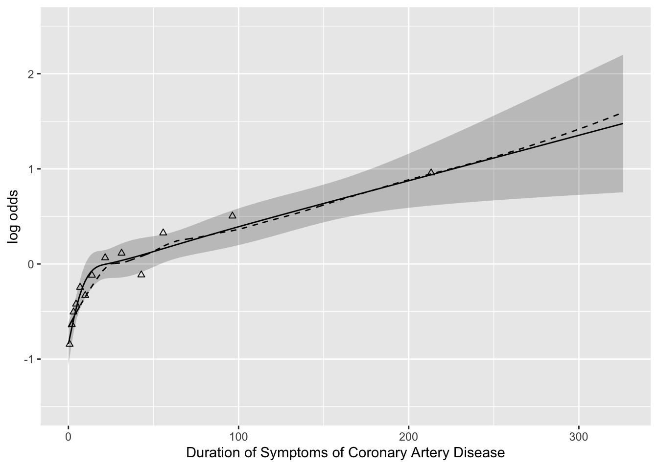
Code
f <- lrm(tvdlm ~ log10(cad.dur + 1), data=d)
binned <- d[, .(prop = mean(tvdlm)), by=.(durg)]
ggplot(Predict(f, cad.dur, fun=plogis), ylab='P') +
  geom_point(data=binned, aes(x=durg, y=prop, shape=I(2)))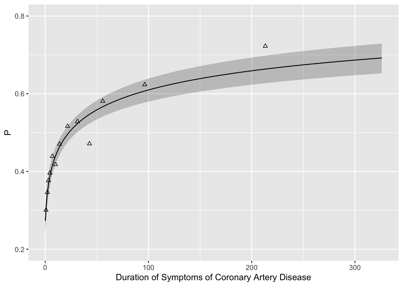
Modeling Interaction Surfaces
W
- Sample of 2258 pts3
- Predict significant coronary disease
- For now stratify age into tertiles to examine interactions simply
- Model has 2 dummies for age, sex, age \(\times\) sex, 4-knot restricted cubic spline in cholesterol, age tertile \(\times\) cholesterol
3 Many patients had missing cholesterol.
Code
acath <- transform(acath,
                   cholesterol = choleste,
                   age.tertile = cut2(age, g=3),
                   sx = as.integer(acath$sex) - 1)
# sx for loess, need to code as numeric
dd <- datadist(acath); options(datadist='dd')

# First model stratifies age into tertiles to get more
# empirical estimates of age x cholesterol interaction

f <- lrm(sigdz ~ age.tertile*(sex + rcs(cholesterol,4)),
         data=acath)
f
Logistic Regression Model
lrm(formula = sigdz ~ age.tertile * (sex + rcs(cholesterol, 4)),
    data = acath)
Frequencies of Missing Values Due to Each Variable sigdz age.tertile sex cholesterol
0 0 0 1246
| Model Likelihood Ratio Test |
Discrimination Indexes |
Rank Discrim. Indexes |
|
|---|---|---|---|
| Obs 2258 | LR χ2 533.52 | R2 0.291 | C 0.780 |
| 0 768 | d.f. 14 | R214,2258 0.206 | Dxy 0.560 |
| 1 1490 | Pr(>χ2) <0.0001 | R214,1520.4 0.289 | γ 0.560 |
| max |∂log L/∂β| 2×10⁻⁸ | Brier 0.173 | τa 0.251 |
| β | S.E. | Wald Z | Pr(>|Z|) | |
|---|---|---|---|---|
| Intercept | -0.4155 | 1.0987 | -0.38 | 0.7053 |
| age.tertile=[49,58) | 0.8781 | 1.7337 | 0.51 | 0.6125 |
| age.tertile=[58,82] | 4.7861 | 1.8143 | 2.64 | 0.0083 |
| sex=female | -1.6123 | 0.1751 | -9.21 | <0.0001 |
| cholesterol | 0.0029 | 0.0060 | 0.48 | 0.6347 |
| cholesterol' | 0.0384 | 0.0242 | 1.59 | 0.1126 |
| cholesterol'' | -0.1148 | 0.0768 | -1.49 | 0.1350 |
| age.tertile=[49,58) × sex=female | -0.7900 | 0.2537 | -3.11 | 0.0018 |
| age.tertile=[58,82] × sex=female | -0.4530 | 0.2978 | -1.52 | 0.1283 |
| age.tertile=[49,58) × cholesterol | 0.0011 | 0.0095 | 0.11 | 0.9093 |
| age.tertile=[58,82] × cholesterol | -0.0158 | 0.0099 | -1.59 | 0.1111 |
| age.tertile=[49,58) × cholesterol' | -0.0183 | 0.0365 | -0.50 | 0.6162 |
| age.tertile=[58,82] × cholesterol' | 0.0127 | 0.0406 | 0.31 | 0.7550 |
| age.tertile=[49,58) × cholesterol'' | 0.0582 | 0.1140 | 0.51 | 0.6095 |
| age.tertile=[58,82] × cholesterol'' | -0.0092 | 0.1301 | -0.07 | 0.9436 |
Code
ltx(f)\[X\hat{\beta}=\]
\[\begin{array}{l} -0.415\\ +0.878[\mathrm{age.tertile} \in [49,58)]+4.79 [\mathrm{age.tertile} \in [58,82]]\\ -1.61[\mathrm{female}]\\+ 0.00287 \mathrm{cholesterol}+1.52\!\times\!10^{-6 }(\mathrm{cholesterol}-160)_{+}^{3} \\ -4.53\!\times\!10^{-6}(\mathrm{cholesterol}-208)_{+}^{3}+3.44\!\times\!10^{-6 }(\mathrm{cholesterol}-243)_{+}^{3} \\ -4.28\!\times\!10^{-7}(\mathrm{cholesterol}-319)_{+}^{3} \\+[\mathrm{female}][-0.79 \:[\mathrm{age.tertile} \in [49,58)]\\ -0.453\:[\mathrm{age.tertile} \in [58,82]] ]\\ +[\mathrm{age.tertile} \in [49,58)][0.00108 \mathrm{cholesterol} \\ -7.23\!\times\!10^{-7}(\mathrm{cholesterol}-160)_{+}^{3}+2.3\!\times\!10^{-6 }(\mathrm{cholesterol}-208)_{+}^{3} \\ -1.84\!\times\!10^{-6}(\mathrm{cholesterol}-243)_{+}^{3}+2.69\!\times\!10^{-7 }(\mathrm{cholesterol}-319)_{+}^{3} ]\\ +[\mathrm{age.tertile} \in [58,82]][-0.0158 \mathrm{cholesterol} \\ +5\!\times\!10^{-7 }(\mathrm{cholesterol}-160)_{+}^{3}-3.64\!\times\!10^{-7}(\mathrm{cholesterol}-208)_{+}^{3} \\ -5.15\!\times\!10^{-7}(\mathrm{cholesterol}-243)_{+}^{3}+3.78\!\times\!10^{-7 }(\mathrm{cholesterol}-319)_{+}^{3} ] \end{array}\]Code
print(anova(f), caption='Crudely categorizing age into tertiles')| Crudely categorizing age into tertiles | |||
| χ2 | d.f. | P | |
|---|---|---|---|
| age.tertile (Factor+Higher Order Factors) | 120.74 | 10 | <0.0001 |
| All Interactions | 21.87 | 8 | 0.0052 |
| sex (Factor+Higher Order Factors) | 329.54 | 3 | <0.0001 |
| All Interactions | 9.78 | 2 | 0.0075 |
| cholesterol (Factor+Higher Order Factors) | 93.75 | 9 | <0.0001 |
| All Interactions | 10.03 | 6 | 0.1235 |
| Nonlinear (Factor+Higher Order Factors) | 9.96 | 6 | 0.1263 |
| age.tertile × sex (Factor+Higher Order Factors) | 9.78 | 2 | 0.0075 |
| age.tertile × cholesterol (Factor+Higher Order Factors) | 10.03 | 6 | 0.1235 |
| Nonlinear | 2.62 | 4 | 0.6237 |
| Nonlinear Interaction : f(A,B) vs. AB | 2.62 | 4 | 0.6237 |
| TOTAL NONLINEAR | 9.96 | 6 | 0.1263 |
| TOTAL INTERACTION | 21.87 | 8 | 0.0052 |
| TOTAL NONLINEAR + INTERACTION | 29.67 | 10 | 0.0010 |
| TOTAL | 410.75 | 14 | <0.0001 |
Code
yl <- c(-1,5)
ggplot(Predict(f, cholesterol, age.tertile),
       adj.subtitle=FALSE, ylim=yl)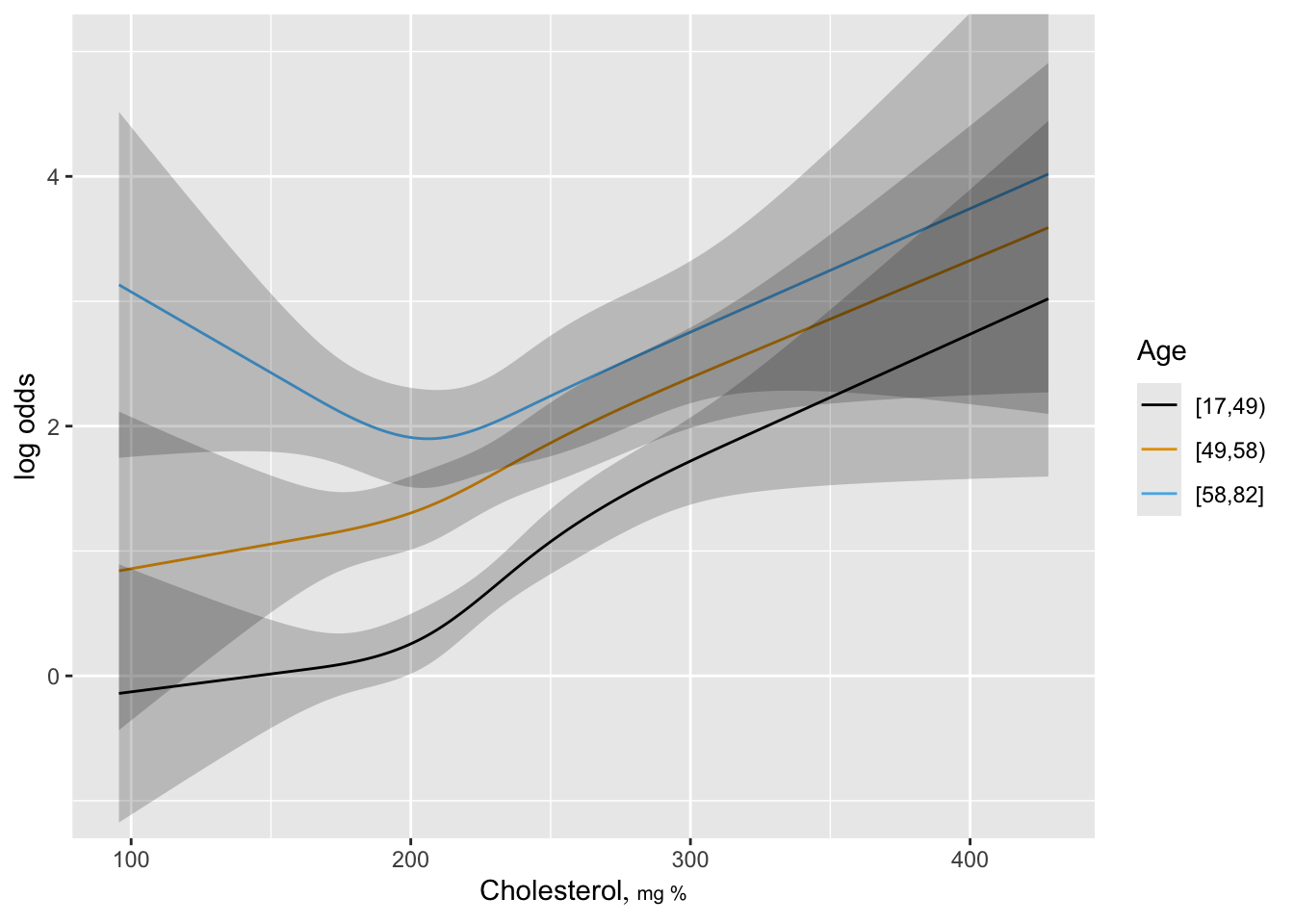
- Now model age as continuous predictor
- Start with nonparametric surface using \(Y=0/1\)
X
Code
# Re-do model with continuous age
require(lattice)   # provides wireframe
f <- loess(sigdz ~ age * (sx + cholesterol), data=acath,
           parametric="sx", drop.square="sx")
ages  <- seq(25,   75, length=40)
chols <- seq(100, 400, length=40)
g <- expand.grid(cholesterol=chols, age=ages, sx=0)
# drop sex dimension of grid since held to 1 value
p <- drop(predict(f, g))
p[p < 0.001] <- 0.001
p[p > 0.999] <- 0.999
zl <- c(-3, 6)
wireframe(qlogis(p) ~ cholesterol*age,
          xlab=list(rot=30), ylab=list(rot=-40),
          zlab=list(label='log odds', rot=90), zlim=zl,
          scales = list(arrows = FALSE), data=g)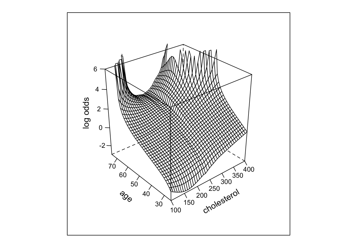
loess function.
- Next try parametric fit using linear spline in age, chol. (3 knots each), all product terms. For all the remaining 3-d plots we limit plotting to points that are supported by at least 5 subjects beyond those cholesterol/age combinations
Y
Code
f <- lrm(sigdz ~ lsp(age,c(46,52,59)) *
         (sex + lsp(cholesterol,c(196,224,259))),
         data=acath)
ltx(f)
\[X\hat{\beta}=\]
\[\begin{array}{l} -1.83\\ +0.0232 \:\mathrm{age}+0.0759 (\mathrm{age}-46)_{+}-0.0025(\mathrm{age}-52)_{+}+2.27 (\mathrm{age}-59)_{+}\\ +3.02[\mathrm{female}]\\ -0.0177\:\mathrm{cholesterol}+0.114 (\mathrm{cholesterol}-196)_{+}\\ -0.131 (\mathrm{cholesterol}-224)_{+}+0.0651 (\mathrm{cholesterol}-259)_{+}\\+[\mathrm{female}][-0.112 \:\mathrm{age}+0.0852 \:(\mathrm{age}-46)_{+}-0.0302\:(\mathrm{age}-52)_{+}\\ +0.176 \:(\mathrm{age}-59)_{+} ]\\+\mathrm{age}[0.000577 \:\mathrm{cholesterol}-0.00286 \:(\mathrm{cholesterol}-196)_{+}\\+0.00382 \:(\mathrm{cholesterol}-224)_{+}-0.00205 \:(\mathrm{cholesterol}-259)_{+} ]\\+(\mathrm{age}-46)_{+}[-0.000936\:\mathrm{cholesterol}+0.00643 \:(\mathrm{cholesterol}-196)_{+}\\-0.0115 \:(\mathrm{cholesterol}-224)_{+}+0.00756 \:(\mathrm{cholesterol}-259)_{+} ]\\+(\mathrm{age}-52)_{+}[0.000433 \:\mathrm{cholesterol}-0.0037 \:(\mathrm{cholesterol}-196)_{+}\\+0.00815 \:(\mathrm{cholesterol}-224)_{+}-0.00715 \:(\mathrm{cholesterol}-259)_{+} ]\\+(\mathrm{age}-59)_{+}[-0.0124 \:\mathrm{cholesterol}+0.015 \:(\mathrm{cholesterol}-196)_{+}\\ -0.0067 \:(\mathrm{cholesterol}-224)_{+}+0.00752 \:(\mathrm{cholesterol}-259)_{+} ] \end{array}\]Code
print(anova(f), caption='Linear spline surface')| Linear spline surface | |||
| χ2 | d.f. | P | |
|---|---|---|---|
| age (Factor+Higher Order Factors) | 164.17 | 24 | <0.0001 |
| All Interactions | 42.28 | 20 | 0.0025 |
| Nonlinear (Factor+Higher Order Factors) | 25.21 | 18 | 0.1192 |
| sex (Factor+Higher Order Factors) | 343.80 | 5 | <0.0001 |
| All Interactions | 23.90 | 4 | <0.0001 |
| cholesterol (Factor+Higher Order Factors) | 100.13 | 20 | <0.0001 |
| All Interactions | 16.27 | 16 | 0.4341 |
| Nonlinear (Factor+Higher Order Factors) | 16.35 | 15 | 0.3595 |
| age × sex (Factor+Higher Order Factors) | 23.90 | 4 | <0.0001 |
| Nonlinear | 12.97 | 3 | 0.0047 |
| Nonlinear Interaction : f(A,B) vs. AB | 12.97 | 3 | 0.0047 |
| age × cholesterol (Factor+Higher Order Factors) | 16.27 | 16 | 0.4341 |
| Nonlinear | 11.45 | 15 | 0.7204 |
| Nonlinear Interaction : f(A,B) vs. AB | 11.45 | 15 | 0.7204 |
| f(A,B) vs. Af(B) + Bg(A) | 9.38 | 9 | 0.4033 |
| Nonlinear Interaction in age vs. Af(B) | 9.99 | 12 | 0.6167 |
| Nonlinear Interaction in cholesterol vs. Bg(A) | 10.75 | 12 | 0.5503 |
| TOTAL NONLINEAR | 33.22 | 24 | 0.0995 |
| TOTAL INTERACTION | 42.28 | 20 | 0.0025 |
| TOTAL NONLINEAR + INTERACTION | 49.03 | 26 | 0.0041 |
| TOTAL | 449.26 | 29 | <0.0001 |
Code
perim <- with(acath,
              perimeter(cholesterol, age, xinc=20, n=5))
zl <- c(-2, 4)
bplot(Predict(f, cholesterol, age, np=40), perim=perim,
      lfun=wireframe, zlim=zl, adj.subtitle=FALSE)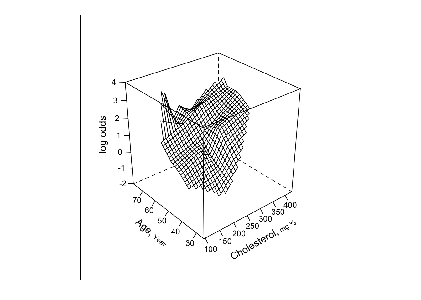
- Next try smooth spline surface, include all cross-products
Z
Code
f <- lrm(sigdz ~ rcs(age,4)*(sex + rcs(cholesterol,4)),
         data=acath)
ltx(f)
\[X\hat{\beta}=\]
\[\begin{array}{l} -6.41\\+ 0.166 \mathrm{age}-0.00067(\mathrm{age}-36)_{+}^{3}+0.00543 (\mathrm{age}-48)_{+}^{3} \\ -0.00727(\mathrm{age}-56)_{+}^{3}+0.00251 (\mathrm{age}-68)_{+}^{3} \\ +2.87[\mathrm{female}]\\+ 0.00979 \mathrm{cholesterol}+1.96\!\times\!10^{-6 }(\mathrm{cholesterol}-160)_{+}^{3} \\ -7.16\!\times\!10^{-6}(\mathrm{cholesterol}-208)_{+}^{3}+6.35\!\times\!10^{-6 }(\mathrm{cholesterol}-243)_{+}^{3} \\ -1.16\!\times\!10^{-6}(\mathrm{cholesterol}-319)_{+}^{3} \\ +[\mathrm{female}][-0.109 \mathrm{age}+7.52\!\times\!10^{-5}(\mathrm{age}-36)_{+}^{3}+0.00015 (\mathrm{age}-48)_{+}^{3} \\ -0.00045(\mathrm{age}-56)_{+}^{3}+0.000225(\mathrm{age}-68)_{+}^{3} ]\\ +\mathrm{age}[-0.00028 \mathrm{cholesterol}+2.68\!\times\!10^{-9 }(\mathrm{cholesterol}-160)_{+}^{3} \\ +3.03\!\times\!10^{-8 }(\mathrm{cholesterol}-208)_{+}^{3}-4.99\!\times\!10^{-8}(\mathrm{cholesterol}-243)_{+}^{3} \\ +1.69\!\times\!10^{-8 }(\mathrm{cholesterol}-319)_{+}^{3} ]\\ +\mathrm{age}'[0.00341 \mathrm{cholesterol}-4.02\!\times\!10^{-7}(\mathrm{cholesterol}-160)_{+}^{3} \\ +9.71\!\times\!10^{-7 }(\mathrm{cholesterol}-208)_{+}^{3}-5.79\!\times\!10^{-7}(\mathrm{cholesterol}-243)_{+}^{3} \\ +8.79\!\times\!10^{-9 }(\mathrm{cholesterol}-319)_{+}^{3} ]\\ +\mathrm{age}''[-0.029 \mathrm{cholesterol}+3.04\!\times\!10^{-6 }(\mathrm{cholesterol}-160)_{+}^{3} \\ -7.34\!\times\!10^{-6}(\mathrm{cholesterol}-208)_{+}^{3}+4.36\!\times\!10^{-6 }(\mathrm{cholesterol}-243)_{+}^{3} \\ -5.82\!\times\!10^{-8}(\mathrm{cholesterol}-319)_{+}^{3} ] \end{array}\]Code
print(anova(f), caption='Cubic spline surface')| Cubic spline surface | |||
| χ2 | d.f. | P | |
|---|---|---|---|
| age (Factor+Higher Order Factors) | 165.23 | 15 | <0.0001 |
| All Interactions | 37.32 | 12 | 0.0002 |
| Nonlinear (Factor+Higher Order Factors) | 21.01 | 10 | 0.0210 |
| sex (Factor+Higher Order Factors) | 343.67 | 4 | <0.0001 |
| All Interactions | 23.31 | 3 | <0.0001 |
| cholesterol (Factor+Higher Order Factors) | 97.50 | 12 | <0.0001 |
| All Interactions | 12.95 | 9 | 0.1649 |
| Nonlinear (Factor+Higher Order Factors) | 13.62 | 8 | 0.0923 |
| age × sex (Factor+Higher Order Factors) | 23.31 | 3 | <0.0001 |
| Nonlinear | 13.37 | 2 | 0.0013 |
| Nonlinear Interaction : f(A,B) vs. AB | 13.37 | 2 | 0.0013 |
| age × cholesterol (Factor+Higher Order Factors) | 12.95 | 9 | 0.1649 |
| Nonlinear | 7.27 | 8 | 0.5078 |
| Nonlinear Interaction : f(A,B) vs. AB | 7.27 | 8 | 0.5078 |
| f(A,B) vs. Af(B) + Bg(A) | 5.41 | 4 | 0.2480 |
| Nonlinear Interaction in age vs. Af(B) | 6.44 | 6 | 0.3753 |
| Nonlinear Interaction in cholesterol vs. Bg(A) | 6.27 | 6 | 0.3931 |
| TOTAL NONLINEAR | 29.22 | 14 | 0.0097 |
| TOTAL INTERACTION | 37.32 | 12 | 0.0002 |
| TOTAL NONLINEAR + INTERACTION | 45.41 | 16 | 0.0001 |
| TOTAL | 450.88 | 19 | <0.0001 |
Code
bplot(Predict(f, cholesterol, age, np=40), perim=perim,
      lfun=wireframe, zlim=zl, adj.subtitle=FALSE)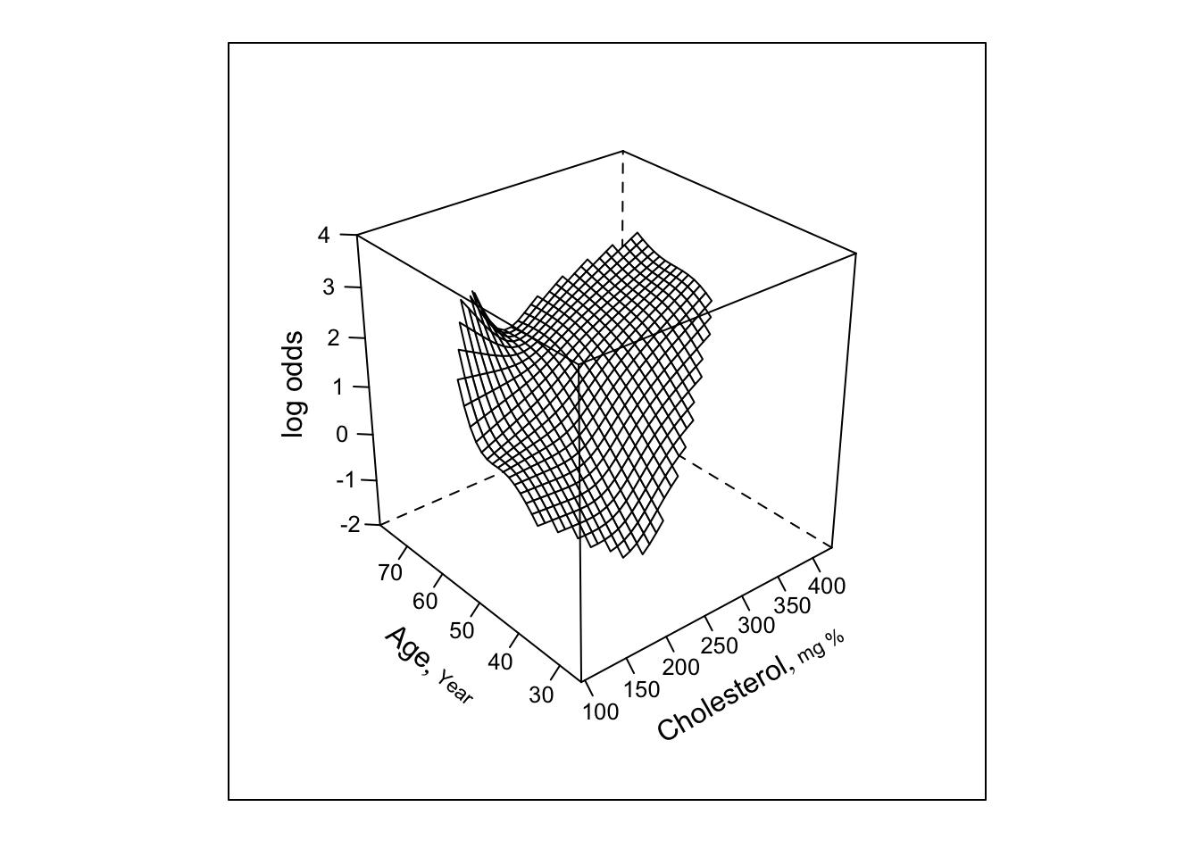
- Now restrict surface by excluding doubly nonlinear terms
A
Code
f <- lrm(sigdz ~ sex*rcs(age,4) + rcs(cholesterol,4) +
         rcs(age,4) %ia% rcs(cholesterol,4), data=acath)
ltx(f)
\[X\hat{\beta}=\]
\[\begin{array}{l} -7.2\\ +2.96[\mathrm{female}]\\+ 0.164 \mathrm{age}+7.23\!\times\!10^{-5 }(\mathrm{age}-36)_{+}^{3}-0.000106(\mathrm{age}-48)_{+}^{3} \\ -1.63\!\times\!10^{-5}(\mathrm{age}-56)_{+}^{3}+4.99\!\times\!10^{-5 }(\mathrm{age}-68)_{+}^{3} \\+ 0.0148 \mathrm{cholesterol}+1.21\!\times\!10^{-6 }(\mathrm{cholesterol}-160)_{+}^{3} \\ -5.5\!\times\!10^{-6 }(\mathrm{cholesterol}-208)_{+}^{3}+5.5\!\times\!10^{-6 }(\mathrm{cholesterol}-243)_{+}^{3} \\ -1.21\!\times\!10^{-6}(\mathrm{cholesterol}-319)_{+}^{3} \\ +\mathrm{age}[-0.00029 \mathrm{cholesterol}+9.28\!\times\!10^{-9 }(\mathrm{cholesterol}-160)_{+}^{3} \\ +1.7\!\times\!10^{-8 }(\mathrm{cholesterol}-208)_{+}^{3}-4.43\!\times\!10^{-8}(\mathrm{cholesterol}-243)_{+}^{3} \\ +1.79\!\times\!10^{-8 }(\mathrm{cholesterol}-319)_{+}^{3} ]\\ +\mathrm{cholesterol}[2.3\!\times\!10^{-7 }(\mathrm{age}-36)_{+}^{3}+4.21\!\times\!10^{-7 }(\mathrm{age}-48)_{+}^{3} \\ -1.31\!\times\!10^{-6}(\mathrm{age}-56)_{+}^{3}+6.64\!\times\!10^{-7 }(\mathrm{age}-68)_{+}^{3} ]\\ +[\mathrm{female}][-0.111 \mathrm{age}+8.03\!\times\!10^{-5}(\mathrm{age}-36)_{+}^{3}+0.000135(\mathrm{age}-48)_{+}^{3} \\ -0.00044(\mathrm{age}-56)_{+}^{3}+0.000224(\mathrm{age}-68)_{+}^{3} ] \end{array}\]Code
print(anova(f),
caption='Singly nonlinear cubic spline surface')| Singly nonlinear cubic spline surface | |||
| χ2 | d.f. | P | |
|---|---|---|---|
| sex (Factor+Higher Order Factors) | 343.42 | 4 | <0.0001 |
| All Interactions | 24.05 | 3 | <0.0001 |
| age (Factor+Higher Order Factors) | 169.35 | 11 | <0.0001 |
| All Interactions | 34.80 | 8 | <0.0001 |
| Nonlinear (Factor+Higher Order Factors) | 16.55 | 6 | 0.0111 |
| cholesterol (Factor+Higher Order Factors) | 93.62 | 8 | <0.0001 |
| All Interactions | 10.83 | 5 | 0.0548 |
| Nonlinear (Factor+Higher Order Factors) | 10.87 | 4 | 0.0281 |
| age × cholesterol (Factor+Higher Order Factors) | 10.83 | 5 | 0.0548 |
| Nonlinear | 3.12 | 4 | 0.5372 |
| Nonlinear Interaction : f(A,B) vs. AB | 3.12 | 4 | 0.5372 |
| Nonlinear Interaction in age vs. Af(B) | 1.60 | 2 | 0.4496 |
| Nonlinear Interaction in cholesterol vs. Bg(A) | 1.64 | 2 | 0.4400 |
| sex × age (Factor+Higher Order Factors) | 24.05 | 3 | <0.0001 |
| Nonlinear | 13.58 | 2 | 0.0011 |
| Nonlinear Interaction : f(A,B) vs. AB | 13.58 | 2 | 0.0011 |
| TOTAL NONLINEAR | 27.89 | 10 | 0.0019 |
| TOTAL INTERACTION | 34.80 | 8 | <0.0001 |
| TOTAL NONLINEAR + INTERACTION | 45.45 | 12 | <0.0001 |
| TOTAL | 453.10 | 15 | <0.0001 |
Code
bplot(Predict(f, cholesterol, age, np=40), perim=perim,
      lfun=wireframe, zlim=zl, adj.subtitle=FALSE)
- Finally restrict the interaction to be a simple product
B
Code
f <- lrm(sigdz ~ rcs(age,4)*sex + rcs(cholesterol,4) +
         age %ia% cholesterol, data=acath)
ltx(f)
\[X\hat{\beta}=\]
\[\begin{array}{l} -7.36\\+ 0.182 \mathrm{age}-5.18\!\times\!10^{-5}(\mathrm{age}-36)_{+}^{3}+8.45\!\times\!10^{-5 }(\mathrm{age}-48)_{+}^{3} \\ -2.91\!\times\!10^{-6}(\mathrm{age}-56)_{+}^{3}-2.99\!\times\!10^{-5}(\mathrm{age}-68)_{+}^{3} \\ +2.8[\mathrm{female}]\\+ 0.0139 \mathrm{cholesterol}+1.76\!\times\!10^{-6 }(\mathrm{cholesterol}-160)_{+}^{3} \\ -4.88\!\times\!10^{-6}(\mathrm{cholesterol}-208)_{+}^{3}+3.45\!\times\!10^{-6 }(\mathrm{cholesterol}-243)_{+}^{3} \\ -3.26\!\times\!10^{-7}(\mathrm{cholesterol}-319)_{+}^{3} \\ -0.00034\:\mathrm{age}\:\times\:\mathrm{cholesterol}\\ +[\mathrm{female}][-0.107 \mathrm{age}+7.71\!\times\!10^{-5 }(\mathrm{age}-36)_{+}^{3}+0.000115 (\mathrm{age}-48)_{+}^{3} \\ -0.000398(\mathrm{age}-56)_{+}^{3}+0.000205 (\mathrm{age}-68)_{+}^{3} ] \end{array}\]Code
print(anova(f), caption='Linear interaction surface')| Linear interaction surface | |||
| χ2 | d.f. | P | |
|---|---|---|---|
| age (Factor+Higher Order Factors) | 167.83 | 7 | <0.0001 |
| All Interactions | 31.03 | 4 | <0.0001 |
| Nonlinear (Factor+Higher Order Factors) | 14.58 | 4 | 0.0057 |
| sex (Factor+Higher Order Factors) | 345.88 | 4 | <0.0001 |
| All Interactions | 22.30 | 3 | <0.0001 |
| cholesterol (Factor+Higher Order Factors) | 89.37 | 4 | <0.0001 |
| All Interactions | 7.99 | 1 | 0.0047 |
| Nonlinear | 10.65 | 2 | 0.0049 |
| age × cholesterol (Factor+Higher Order Factors) | 7.99 | 1 | 0.0047 |
| age × sex (Factor+Higher Order Factors) | 22.30 | 3 | <0.0001 |
| Nonlinear | 12.06 | 2 | 0.0024 |
| Nonlinear Interaction : f(A,B) vs. AB | 12.06 | 2 | 0.0024 |
| TOTAL NONLINEAR | 25.72 | 6 | 0.0003 |
| TOTAL INTERACTION | 31.03 | 4 | <0.0001 |
| TOTAL NONLINEAR + INTERACTION | 43.59 | 8 | <0.0001 |
| TOTAL | 452.75 | 11 | <0.0001 |
Code
bplot(Predict(f, cholesterol, age, np=40), perim=perim,
      lfun=wireframe, zlim=zl, adj.subtitle=FALSE)
f.linia <- f  # save linear interaction fit for later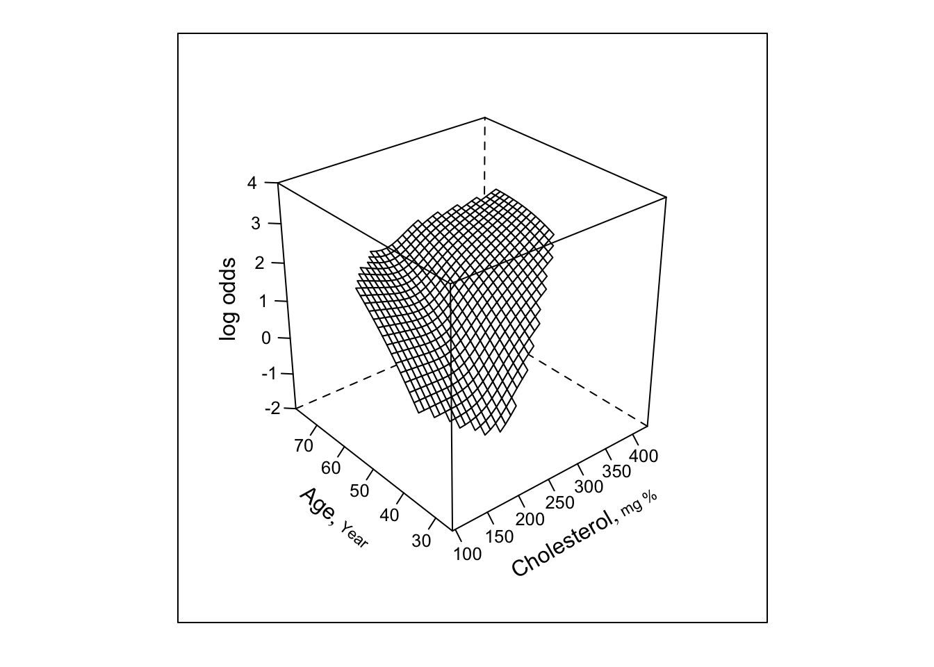
The Wald test for age \(\times\) cholesterol interaction yields \(\chi^{2}=7.99\) with 1 d.f., p=.005. * See how well this simple interaction model compares with initial model using 2 dummies for age * Request predictions to be made at mean age within tertiles
C
Code
# Make estimates of cholesterol effects for mean age in
# tertiles corresponding to initial analysis
mean.age <-
  with(acath,
       as.vector(tapply(age, age.tertile, mean, na.rm=TRUE)))
mean.age <- unique(mb(acath$age, g=3))
ggplot(Predict(f, cholesterol, age=round(mean.age, 2),
             sex="male"),
     adj.subtitle=FALSE, ylim=yl) #3 curves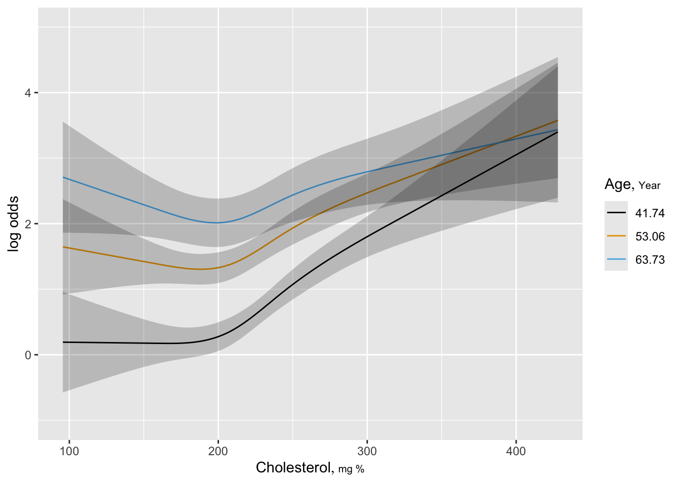
- Using residuals for “duration of symptoms” example
Code
spar(mfrow=c(1,2), ps=10)
f <- lrm(tvdlm ~ cad.dur, data=d, x=TRUE, y=TRUE)
resid(f, "partial", pl="loess", xlim=c(0,250), ylim=c(-3,3))
scat1d(d$cad.dur)
log.cad.dur <- log10(d$cad.dur + 1)
f <- lrm(tvdlm ~ log.cad.dur, data=d, x=TRUE, y=TRUE)
resid(f, "partial", pl="loess", ylim=c(-3,3))
scat1d(log.cad.dur)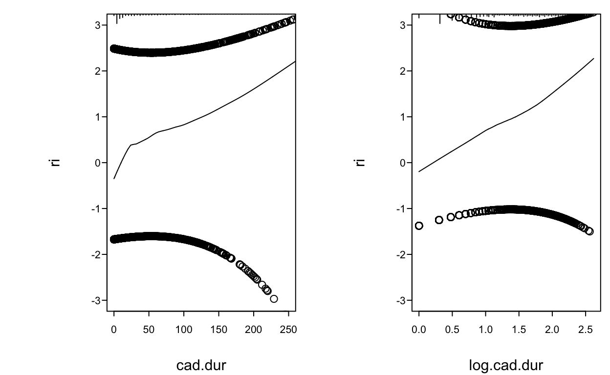
- Relative merits of strat., nonparametric, splines for checking fit
D
| Method | Choice Required | Assumes Additivity | Uses Ordering of \(X\) | Low Variance | Good Resolution on \(X\) |
|---|---|---|---|---|---|
| Stratification | Intervals | ||||
| Smoother on \(X_{1}\) stratifying on \(X_{2}\) | Bandwidth | × (not on \(X_2\)) | × (if min. strat.) | × (\(X_1\)) | |
| Smooth partial residual plot | Bandwidth | × | × | × | × |
| Spline model for all \(X\)x | Knots | × | × | × | × |
- Hosmer-Lemeshow test is a commonly used test of goodness-of-fit of a binary logistic model
Compares proportion of events with mean predicted probability within deciles of \(\hat{P}\)- Arbitrary (number of groups, how to form groups)
- Low power (too many d.f.)
- Does not reveal the culprits
- A new omnibus test based of SSE has more power and requires no grouping; still does not lead to corrective action.
- Any omnibus test lacks power against specific alternatives such as nonlinearity or interaction
E
10.6 Collinearity
10.7 Overly Influential Observations
10.8 Quantifying Predictive Ability
F
Generalized Nagelkerke \(R^2\): equals ordinary \(R^2\) in normal case: \[ R^{2}_{\rm N} = \frac{1 - \exp(-{\rm LR}/n)}{1 - \exp(-L^{0}/n)}, \]
4 versions of Maddala-Cox-Snell \(R^2\): hbiostat.org/bib/r2.html
- Perhaps best: \(R^{2}_{p,m} = 1 - \exp(-({\rm LR} - p) / m)\)
- \(m\) is the effective sample size based on approximate variance of a log odds ratio in a proportional odds ordinal logistic model
- If \(Y\) has \(k\) distinct values with proportions \(p_{1}, p_{2}, \ldots, p_{k}\),
\(m=n \times (1 - \sum_{i=1}^{k}p_{i}^{3})\) - For binary \(Y\) with proportion \(Y=1\) of \(p\),
\(m=n\times 3p(1-p)\)
With perfect prediction in the case where there are 50 \(X=0\) and 50 \(X=1\) with \(Y=X\), \(R^{2}_{N}=1, R^{2}_{n,0}=0.75, R^{2}_{m,0}=0.84\)
Brier score (calibration + discrimination): \[ B = \frac{1}{n} \sum_{i=1}^{n} (\hat{P}_{i} - Y_{i})^{2}, \]
\(c\) = “concordance probability” = ROC area
- Related to Wilcoxon-Mann-Whitney stat and Somers’ \(D_{xy}\) \[ D_{xy} = 2 (c-.5) . \]
- Good pure index of predictive discrimination for a single model
- Not useful for comparing two models (Cook, 2007; Pencina et al., 2008)4
“Coefficient of discrimination” (Tjur, 2009): average \(\hat{P}\) when \(Y=1\) minus average \(\hat{P}\) when \(Y=0\)
- Has many advantages. Tjur shows how it ties in with sum of squares–based \(R^{2}\) measures.
“Percent classified correctly” has lots of problems
- improper scoring rule; optimizing it will lead to incorrect model
- arbitrary, insensitive, uses a strange loss (utility function)
10.9 Validating the Fitted Model
I
- Possible indexes (Austin & Steyerberg, 2019)
- Accuracy of \(\hat{P}\): calibration
Plot \(\text{expit}(X_{new}\hat{\beta}_{old})\) against estimated \(\Pr(Y=1)\) on new data - Discrimination: \(C\) or \(D_{xy}\)
- \(R^2\) or \(B\)
- Accuracy of \(\hat{P}\): calibration
- Use bootstrap to estimate calibration equation \[ P_{c} = \Pr(Y=1 | X\hat{\beta}) = \text{expit}(\gamma_{0} + \gamma_{1} X\hat{\beta}) \] \[ E_{max}(a,b) = \max_{a \leq \hat{P} \leq b} |\hat{P} - \hat{P}_{c}| , \]
- Bootstrap validation of age-sex-response data, 150 samples
- 2 predictors forced into every model
J
Code
require(rms)
getHdata(sex.age.response)
d  <- sex.age.response
dd <- datadist(d); options(datadist='dd')
f  <- lrm(response ~ sex + age, data=d, x=TRUE, y=TRUE)
set.seed(3)  # for reproducibility
# Some bootstrap samples had complete separation (infinite beta) in which case
# the default convergence criteria results in too many iterations.  Specify
# absolute tolerance to avoid this.
v1  <- validate(f, B=150, maxit=20)
ap1 <- round(v1[,'index.orig']     , 2)
bc1 <- round(v1[,'index.corrected'], 2)
print(v1,
      caption='Bootstrap Validation, 2 Predictors Without Stepdown',
digits=2)| Bootstrap Validation, 2 Predictors Without Stepdown | ||||||||
| Index | Original Sample |
Training Sample |
Test Sample |
Optimism | Corrected Index |
Lower | Upper | Successful Resamples |
|---|---|---|---|---|---|---|---|---|
| Dxy | 0.7 | 0.7 | 0.67 | 0.03 | 0.66 | 0.45 | 0.94 | 150 |
| R2 | 0.45 | 0.48 | 0.43 | 0.05 | 0.4 | 0.11 | 0.69 | 150 |
| Intercept | 0 | 0 | 0.04 | -0.04 | 0.04 | -0.93 | 1.03 | 150 |
| Slope | 1 | 1 | 0.92 | 0.08 | 0.92 | 0.25 | 1.88 | 150 |
| Emax | 0 | 0 | 0.13 | -0.13 | 0.13 | -0.03 | 0.34 | 150 |
| D | 0.39 | 0.43 | 0.36 | 0.07 | 0.32 | -0.05 | 0.64 | 150 |
| U | -0.05 | -0.05 | 0.02 | -0.07 | 0.02 | -0.11 | 0.41 | 150 |
| Q | 0.44 | 0.48 | 0.34 | 0.14 | 0.3 | -0.39 | 0.66 | 150 |
| B | 0.16 | 0.15 | 0.18 | -0.03 | 0.19 | 0.12 | 0.28 | 150 |
| g | 2.1 | 2.38 | 1.97 | 0.41 | 1.7 | -0.71 | 3.15 | 150 |
| gp | 0.35 | 0.35 | 0.34 | 0.01 | 0.34 | 0.23 | 0.48 | 150 |
- Allow for step-down at each re-sample
- Use individual tests at \(\alpha=0.10\)
- Both age and sex selected in 138 of 150, neither in 1 samples
K
Code
v2 <- validate(f, B=150, bw=TRUE,
               rule='p', sls=.1, type='individual',
               maxit=30)
        Backwards Step-down - Original Model

No Factors Deleted

Factors in Final Model

[1] sex age
Code
ap2 <- round(v2[,'index.orig'], 2)
bc2 <- round(v2[,'index.corrected'], 2)
print(v2,
      caption='Bootstrap Validation, 2 Predictors with Stepdown',
digits=2, B=15)| Bootstrap Validation, 2 Predictors with Stepdown | ||||||||
| Index | Original Sample |
Training Sample |
Test Sample |
Optimism | Corrected Index |
Lower | Upper | Successful Resamples |
|---|---|---|---|---|---|---|---|---|
| Dxy | 0.7 | 0.71 | 0.65 | 0.07 | 0.63 | 0.39 | 0.88 | 150 |
| R2 | 0.45 | 0.5 | 0.41 | 0.09 | 0.36 | 0.06 | 0.65 | 150 |
| Intercept | 0 | 0 | 0.01 | -0.01 | 0.01 | 149 | ||
| Slope | 1 | 1 | 0.83 | 0.17 | 0.83 | 149 | ||
| Emax | 0 | 0 | 0.14 | -0.14 | 0.14 | 149 | ||
| D | 0.39 | 0.46 | 0.35 | 0.11 | 0.28 | -0.13 | 0.6 | 150 |
| U | -0.05 | -0.05 | 0.05 | -0.1 | 0.05 | -0.13 | 0.66 | 150 |
| Q | 0.44 | 0.51 | 0.29 | 0.21 | 0.22 | -0.71 | 0.66 | 150 |
| B | 0.16 | 0.14 | 0.18 | -0.04 | 0.2 | 0.12 | 0.3 | 150 |
| g | 2.1 | 2.6 | 1.9 | 0.7 | 1.4 | -1.78 | 3.03 | 150 |
| gp | 0.35 | 0.35 | 0.33 | 0.02 | 0.33 | 0.21 | 0.45 | 150 |
| Factors Retained in Backwards Elimination First 15 Resamples |
|
| sex | age |
|---|---|
| ⚬ | ⚬ |
| ⚬ | ⚬ |
| ⚬ | ⚬ |
| ⚬ | |
| ⚬ | ⚬ |
| ⚬ | ⚬ |
| ⚬ | ⚬ |
| ⚬ | ⚬ |
| ⚬ | ⚬ |
| ⚬ | ⚬ |
| ⚬ | ⚬ |
| ⚬ | ⚬ |
| ⚬ | ⚬ |
| ⚬ | ⚬ |
| ⚬ | |
| Frequencies of Numbers of Factors Retained | ||
| 0 | 1 | 2 |
|---|---|---|
| 1 | 11 | 138 |
- Try adding 5 noise candidate variables
L
Code
set.seed(133)
n  <- nrow(d)
x1 <- runif(n)
x2 <- runif(n)
x3 <- runif(n)
x4 <- runif(n)
x5 <- runif(n)
f  <- lrm(response ~ age + sex + x1 + x2 + x3 + x4 + x5,
          data=d, x=TRUE, y=TRUE)
v3 <- validate(f, B=150, bw=TRUE,
               rule='p', sls=.1, type='individual')
        Backwards Step-down - Original Model

 Deleted Chi-Sq d.f. P      Residual d.f. P      AIC
 x1      0.01   1    0.9261 0.01     1    0.9261 -1.99
 x5      0.53   1    0.4650 0.54     2    0.7624 -3.46
 x4      0.74   1    0.3902 1.28     3    0.7337 -4.72
 x2      1.03   1    0.3113 2.31     4    0.6796 -5.69
 x3      0.94   1    0.3333 3.24     5    0.6627 -6.76

Approximate Estimates after Deleting Factors

             Coef    S.E. Wald Z        P
Intercept -8.8187 3.76406 -2.343 0.019136
age        0.1415 0.06469  2.188 0.028698
sex=male   3.1059 1.18103  2.630 0.008544

Factors in Final Model

[1] age sex
Code
ap3 <- round(v3[,'index.orig'], 2)
bc3 <- round(v3[,'index.corrected'], 2)
k <- attr(v3, 'kept')
# Compute number of x1-x5 selected
nx <- apply(k[,3:7], 1, sum)
# Get selections of age and sex
v <- colnames(k)
as <- apply(k[,1:2], 1,
            function(x) paste(v[1:2][x], collapse=', '))
Code
kabl(table(paste(as, ' ', nx, 'Xs')))| 0 Xs | 1 Xs | age, sex 0 Xs | age, sex 1 Xs | age, sex 2 Xs | age, sex 3 Xs | sex 0 Xs | sex 1 Xs | sex 2 Xs |
|---|---|---|---|---|---|---|---|---|
| 64 | 4 | 30 | 26 | 8 | 5 | 9 | 3 | 1 |
Code
print(v3,
      caption='Bootstrap Validation with 5 Noise Variables and Stepdown',
digits=2, B=15)| Bootstrap Validation with 5 Noise Variables and Stepdown | ||||||||
| Index | Original Sample |
Training Sample |
Test Sample |
Optimism | Corrected Index |
Lower | Upper | Successful Resamples |
|---|---|---|---|---|---|---|---|---|
| Dxy | 0.7 | 0.42 | 0.35 | 0.08 | 0.62 | 0.45 | 0.86 | 150 |
| R2 | 0.45 | 0.31 | 0.21 | 0.1 | 0.35 | 0.05 | 0.51 | 150 |
| Intercept | 0 | 0 | 0.07 | -0.07 | 0.07 | 86 | ||
| Slope | 1 | 1 | 0.63 | 0.37 | 0.63 | 86 | ||
| Emax | 0 | 0 | 0.17 | -0.17 | 0.17 | 86 | ||
| D | 0.39 | 0.28 | 0.16 | 0.12 | 0.27 | -0.1 | 0.46 | 150 |
| U | -0.05 | -0.05 | 0.05 | -0.1 | 0.05 | -0.13 | 0.71 | 150 |
| Q | 0.44 | 0.33 | 0.11 | 0.22 | 0.22 | -0.78 | 0.57 | 150 |
| B | 0.16 | 0.18 | 0.22 | -0.04 | 0.2 | 0.15 | 0.28 | 150 |
| g | 2.1 | 1.64 | 0.96 | 0.68 | 1.42 | -1.73 | 2.48 | 150 |
| gp | 0.35 | 0.21 | 0.17 | 0.04 | 0.31 | 0.22 | 0.44 | 150 |
| Factors Retained in Backwards Elimination First 15 Resamples |
||||||
| age | sex | x1 | x2 | x3 | x4 | x5 |
|---|---|---|---|---|---|---|
| ⚬ | ⚬ | |||||
| ⚬ | ⚬ | |||||
| ⚬ | ||||||
| ⚬ | ⚬ | ⚬ | ⚬ | |||
| ⚬ | ⚬ | ⚬ | ||||
| ⚬ | ⚬ | |||||
| ⚬ | ⚬ | ⚬ | ⚬ | ⚬ | ||
| ⚬ | ||||||
| ⚬ | ⚬ | ⚬ | ||||
| ⚬ | ⚬ | ⚬ | ||||
| Frequencies of Numbers of Factors Retained | |||||
| 0 | 1 | 2 | 3 | 4 | 5 |
|---|---|---|---|---|---|
| 64 | 13 | 33 | 27 | 8 | 5 |
- Repeat but force age and sex to be in all models
M
Code
v4 <- validate(f, B=150, bw=TRUE, rule='p', sls=.1,
               type='individual', force=1:2)
        Backwards Step-down - Original Model

Parameters forced into all models:
 age, sex=male

 Deleted Chi-Sq d.f. P      Residual d.f. P      AIC
 x1      0.01   1    0.9261 0.01     1    0.9261 -1.99
 x5      0.53   1    0.4650 0.54     2    0.7624 -3.46
 x4      0.74   1    0.3902 1.28     3    0.7337 -4.72
 x2      1.03   1    0.3113 2.31     4    0.6796 -5.69
 x3      0.94   1    0.3333 3.24     5    0.6627 -6.76

Approximate Estimates after Deleting Factors

             Coef    S.E. Wald Z        P
Intercept -8.8187 3.76406 -2.343 0.019136
age        0.1415 0.06469  2.188 0.028698
sex=male   3.1059 1.18103  2.630 0.008544

Factors in Final Model

[1] age sex
Code
ap4 <- round(v4[,'index.orig'], 2)
bc4 <- round(v4[,'index.corrected'], 2)
Code
print(v4,
      caption='Bootstrap Validation with 5 Noise Variables and Stepdown, Forced Inclusion of age and sex',
digits=2, B=15)| Bootstrap Validation with 5 Noise Variables and Stepdown, Forced Inclusion of age and sex | ||||||||
| Index | Original Sample |
Training Sample |
Test Sample |
Optimism | Corrected Index |
Lower | Upper | Successful Resamples |
|---|---|---|---|---|---|---|---|---|
| Dxy | 0.7 | 0.77 | 0.66 | 0.11 | 0.59 | 0.36 | 0.83 | 150 |
| R2 | 0.45 | 0.55 | 0.42 | 0.13 | 0.32 | 0.01 | 0.6 | 150 |
| Intercept | 0 | 0 | 0.05 | -0.05 | 0.05 | -0.8 | 0.91 | 150 |
| Slope | 1 | 1 | 0.74 | 0.26 | 0.74 | 0.12 | 1.45 | 150 |
| Emax | 0 | 0 | 0.15 | -0.15 | 0.15 | -0.03 | 0.4 | 150 |
| D | 0.39 | 0.51 | 0.35 | 0.16 | 0.22 | -0.17 | 0.56 | 150 |
| U | -0.05 | -0.05 | 0.09 | -0.14 | 0.09 | -0.15 | 1.28 | 150 |
| Q | 0.44 | 0.56 | 0.26 | 0.3 | 0.14 | -1.26 | 0.65 | 150 |
| B | 0.16 | 0.13 | 0.18 | -0.05 | 0.21 | 0.13 | 0.31 | 150 |
| g | 2.1 | 2.88 | 1.91 | 0.97 | 1.13 | -1.88 | 2.87 | 150 |
| gp | 0.35 | 0.38 | 0.34 | 0.04 | 0.31 | 0.18 | 0.43 | 150 |
| Factors Retained in Backwards Elimination First 15 Resamples |
||||||
| age | sex | x1 | x2 | x3 | x4 | x5 |
|---|---|---|---|---|---|---|
| ⚬ | ⚬ | |||||
| ⚬ | ⚬ | |||||
| ⚬ | ⚬ | ⚬ | ||||
| ⚬ | ⚬ | |||||
| ⚬ | ⚬ | ⚬ | ||||
| ⚬ | ⚬ | |||||
| ⚬ | ⚬ | |||||
| ⚬ | ⚬ | |||||
| ⚬ | ⚬ | |||||
| ⚬ | ⚬ | |||||
| ⚬ | ⚬ | |||||
| ⚬ | ⚬ | |||||
| ⚬ | ⚬ | |||||
| ⚬ | ⚬ | |||||
| ⚬ | ⚬ | ⚬ | ||||
| Frequencies of Numbers of Factors Retained | ||||
| 2 | 3 | 4 | 5 | 6 |
|---|---|---|---|---|
| 108 | 29 | 10 | 1 | 2 |
10.10 Describing the Fitted Model
Code
s <- summary(f.linia)
s
Effects Response: sigdz |
|||||||
| Low | High | Δ | Effect | S.E. | Lower 0.95 | Upper 0.95 | |
|---|---|---|---|---|---|---|---|
| age | 46 | 59 | 13 | 0.90630 | 0.1838 | 0.54600 | 1.2670 |
| Odds Ratio | 46 | 59 | 13 | 2.47500 | 1.72600 | 3.5490 | |
| cholesterol | 196 | 259 | 63 | 0.75480 | 0.1364 | 0.48740 | 1.0220 |
| Odds Ratio | 196 | 259 | 63 | 2.12700 | 1.62800 | 2.7790 | |
| sex --- female:male | 1 | 2 | -2.43000 | 0.1484 | -2.72100 | -2.1390 | |
| Odds Ratio | 1 | 2 | 0.08806 | 0.06584 | 0.1178 | ||
Code
plot(s)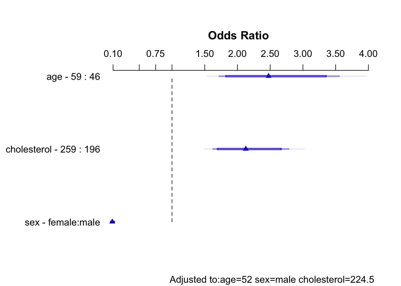
Code
#|label: fig-lrm-iacholxage-3-nomogram
# Draw a nomogram that shows examples of confidence intervals
nom <- nomogram(f.linia, cholesterol=seq(150, 400, by=50),
                interact=list(age=seq(30, 70, by=10)),
                lp.at=seq(-2, 3.5, by=.5),
                conf.int=TRUE, conf.lp="all",
                fun=function(x)1/(1+exp(-x)),  # or plogis
                funlabel="Probability of CAD",
                fun.at=c(seq(.1, .9, by=.1), .95, .99)
                )
plot(nom, col.grid = gray(c(0.8, 0.95)),
     varname.label=FALSE, ia.space=1, xfrac=.46, lmgp=.2)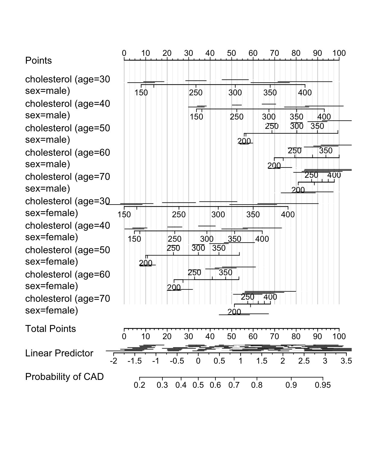
Linear Predictor scale there are various lengths of confidence intervals near the same value of \(X\hat{\beta}\), demonstrating that the standard error of \(X\hat{\beta}\) depends on the individual \(X\) values. Also note that confidence intervals corresponding to smaller patient groups (e.g., females) are wider.10.11 Bayesian Logistic Model Example
Re-analyze data in Section Section 10.1.3 using the R rmsb package. See hbiostat.org/doc/rms/lrm-brms.pdf for a parallel analysis using the brms package. [See this] for detailed examples of Bayesian power and sample size calculations for the PO model]{.aside}
The rmsb package relies on the Stan Bayesian modeling system (Carpenter et al., 2017; Stan Development Team, 2020).
Code
require(rmsb)
dd <- datadist(sex.age.response)
options(datadist = 'dd', mc.cores=4, rmsb.backend='cmdstan')
cmdstanr::set_cmdstan_path(cmdstan.loc)

# Frequentist model
flrm <- lrm(response ~ sex + age, data=sex.age.response)

# Bayesian model

# Fit a model with all flat priors
set.seed(8)
ff <- blrm(response ~ sex + age, data=sex.age.response, iter=5000)
Running MCMC with 4 parallel chains...
Chain 1 finished in 0.1 seconds.
Chain 2 finished in 0.1 seconds.
Chain 3 finished in 0.1 seconds.
Chain 4 finished in 0.1 seconds.
All 4 chains finished successfully.
Mean chain execution time: 0.1 seconds.
Total execution time: 0.3 seconds.Code
# Elapsed time 2.2s
kabl(round(rbind(MLE =coef(flrm), Mode  =coef(ff, 'mode'),
Mean=coef(ff), Median=coef(ff, 'median')), 3))| Intercept | sex=male | age | |
|---|---|---|---|
| MLE | -9.843 | 3.490 | 0.158 |
| Mode | -9.843 | 3.490 | 0.158 |
| Mean | -11.279 | 3.944 | 0.181 |
| Median | -10.958 | 3.836 | 0.176 |
The frequentist model was fitted using lrm and the Bayesian model is fitted using the rmsb blrm function. For the Bayesian model, the intercept prior is non-informative (iprior=1), and flat priors are used for the two slopes. Posterior modes from this fit are in close agreement with the maximum likelihood estimates (MLE) from the frequentist model fit.
For blrm the default prior for non-intercept parameters is a non-informative prior. To use an informative Gaussian prior, the prior is applied to a contrast such as a treatment effect, a slope, or an interaction effect. This is done using the pcontrast argument. The prior for the age effect is set for a 10-year increase log odds for age, and for sex is for a the male - female difference in log odds. Prior standard deviations are computed to satisfied specified tail probabilities. Four MCMC chains with 5000 iterations were used with a warm-up of 2500 iterations each, resulting in 10000 retained draws from the posterior distribution.
Code
# Set priors
# Solve for SD such that sex effect has only a 0.025 chance of
# being above 5 (or being below -5)

s1 <- 5 / qnorm(0.975)

# Solve for SD such that 10-year age effect has only 0.025 chance
# of being above 20

s2 <- 20 / qnorm(0.975)

# Full model
set.seed(11)
. <- function(...) list(...)    # shortcut
pcon <- .(sd=c(s1, s2),
          c1=.(sex='male'), c2=.(sex='female'),
          c3=.(age=30), c4=.(age=20),
          contrast=expression(c1 - c2, c3 - c4) )
f <- blrm(response ~ sex + age, data=sex.age.response,
          pcontrast=pcon, iprior=1, iter=5000)
Running MCMC with 4 parallel chains...
Chain 1 finished in 0.1 seconds.
Chain 2 finished in 0.1 seconds.
Chain 3 finished in 0.1 seconds.
Chain 4 finished in 0.1 seconds.
All 4 chains finished successfully.
Mean chain execution time: 0.1 seconds.
Total execution time: 0.3 seconds.Code
# Elapsed time 1.7s
f
Bayesian Logistic Model
Non-informative Priors for Intercepts
blrm(formula = response ~ sex + age, data = sex.age.response,
    iprior = 1, pcontrast = pcon, iter = 5000)
| Mixed Calibration/ Discrimination Indexes |
Discrimination Indexes |
Rank Discrim. Indexes |
|
|---|---|---|---|
| Obs 40 | LOO log L -22.5±3.36 | g 2.063 [0.884, 3.217] | C 0.835 [0.798, 0.854] |
| 0 20 | LOO IC 44.99±6.71 | gp 0.335 [0.236, 0.428] | Dxy 0.671 [0.597, 0.708] |
| 1 20 | Effective p 2.86±0.61 | EV 0.348 [0.166, 0.544] | |
| Draws 10000 | B 0.175 [0.162, 0.2] | v 3.551 [0.592, 7.777] | |
| Chains 4 | vp 0.086 [0.04, 0.135] | ||
| Time 0.6s | |||
| p 2 |
| Mode β | Mean β | Median β | S.E. | Lower | Upper | Pr(β>0) | Symmetry | |
|---|---|---|---|---|---|---|---|---|
| Intercept | -8.4224 | -9.3774 | -9.1698 | 3.2676 | -16.1688 | -3.4185 | 0.0005 | 0.85 |
| sex=male | 2.9163 | 3.1983 | 3.1457 | 1.0167 | 1.2372 | 5.2432 | 0.9999 | 1.17 |
| age | 0.1362 | 0.1521 | 0.1493 | 0.0561 | 0.0422 | 0.2622 | 0.9985 | 1.15 |
Contrasts Given Priors
[1] "list(sd = c(2.55106728462327, 10.2042691384931), c1 = list(sex = \"male\"), "
[2] "    c2 = list(sex = \"female\"), c3 = list(age = 30), c4 = list("
[3] "        age = 20), contrast = expression(c1 - c2, c3 - c4))"
MCMC sampling diagnostics are below. No apparent problems.
Code
stanDx(f)Iterations: 5000 on each of 4 chains, with 10000 posterior distribution samples saved
For each parameter, n_eff is a crude measure of effective sample size
and Rhat is the potential scale reduction factor on split chains
(at convergence, Rhat=1)
Checking sampler transitions for divergences.
No divergent transitions found.
Checking E-BFMI - sampler transitions HMC potential energy.
E-BFMI satisfactory.
Rank-normalized split effective sample size satisfactory for all parameters.
Rank-normalized split R-hat values satisfactory for all parameters.
Processing complete, no problems detected.
EBFMI: 1.043 1.015 1.066 1.067
Parameter Rhat ESS bulk ESS tail
1 alpha[1] 1.001 7809 7096
2 beta[1] 1.000 6747 5907
3 beta[2] 1.001 6862 6165Code
stanDxplot(f)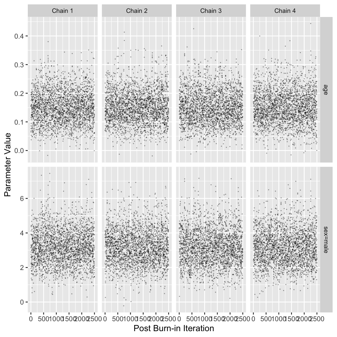
The model summaries for the frequentist and Bayesian models are shown below, with posterior means computed as Bayesian “point estimates.” The parameter estimates are similar for the two approaches. The frequentist 0.95 confidence interval for the age parameter is 0.037 - 0.279 while the Bayesian 0.95 credible interval is 0.044 - 0.265. Similarly, the 0.95 confidence interval for sex is 1.14 - 5.84 and the corresponding Bayesian 0.95 credible interval is 1.23 - 5.28. The results made sense in view of the use of skeptical priors when the sample size is small.
Code
# Frequentist model output
flrm
Logistic Regression Model
lrm(formula = response ~ sex + age, data = sex.age.response)
| Model Likelihood Ratio Test |
Discrimination Indexes |
Rank Discrim. Indexes |
|
|---|---|---|---|
| Obs 40 | LR χ2 16.54 | R2 0.451 | C 0.849 |
| 0 20 | d.f. 2 | R22,40 0.305 | Dxy 0.698 |
| 1 20 | Pr(>χ2) 0.0003 | R22,30 0.384 | γ 0.703 |
| max |∂log L/∂β| 7×10⁻⁸ | Brier 0.162 | τa 0.358 |
| β | S.E. | Wald Z | Pr(>|Z|) | |
|---|---|---|---|---|
| Intercept | -9.8429 | 3.6758 | -2.68 | 0.0074 |
| sex=male | 3.4898 | 1.1992 | 2.91 | 0.0036 |
| age | 0.1581 | 0.0616 | 2.56 | 0.0103 |
Code
summary(flrm, age=20:21)Effects Response: response |
|||||||
| Low | High | Δ | Effect | S.E. | Lower 0.95 | Upper 0.95 | |
|---|---|---|---|---|---|---|---|
| age | 20 | 21 | 1 | 0.1581 | 0.06164 | 0.03725 | 0.2789 |
| Odds Ratio | 20 | 21 | 1 | 1.1710 | 1.03800 | 1.3220 | |
| sex --- male:female | 1 | 2 | 3.4900 | 1.19900 | 1.13900 | 5.8400 | |
| Odds Ratio | 1 | 2 | 32.7800 | 3.12500 | 343.8000 | ||
Code
# Bayesian model output
summary(f, age=20:21)   # posterior means
Effects Response: response |
|||||||
| Low | High | Δ | Effect | S.E. | Lower 0.95 | Upper 0.95 | |
|---|---|---|---|---|---|---|---|
| age | 20 | 21 | 1 | 0.1521 | 0.05613 | 0.04225 | 0.2622 |
| Odds Ratio | 20 | 21 | 1 | 1.1640 | 1.04300 | 1.3000 | |
| sex --- male:female | 1 | 2 | 3.1980 | 1.01700 | 1.23700 | 5.2430 | |
| Odds Ratio | 1 | 2 | 24.4900 | 3.44600 | 189.3000 | ||
Code
summary(f, age=20:21, posterior.summary='median') # post. mediansEffects Response: response |
|||||||
| Low | High | Δ | Effect | S.E. | Lower 0.95 | Upper 0.95 | |
|---|---|---|---|---|---|---|---|
| age | 20 | 21 | 1 | 0.1493 | 0.05613 | 0.04225 | 0.2622 |
| Odds Ratio | 20 | 21 | 1 | 1.1610 | 1.04300 | 1.3000 | |
| sex --- male:female | 1 | 2 | 3.1460 | 1.01700 | 1.23700 | 5.2430 | |
| Odds Ratio | 1 | 2 | 23.2300 | 3.44600 | 189.3000 | ||
Code
# Note that mean vs median doesn't affect HPD intervals, only pt estimatesThe figure shows the posterior draws for the age and sex parameters as well as the trace of the 4 MCMC chains for each parameter and the bivariate posterior distribution. The posterior distributions of each parameter are roughly round shaped and the overlap between chains in the trace plots indicates good convergence. The bivariate density plot indicates moderate correlation between the age and sex parameters.
Create a 0.95 bivariate credible interval for the joint distribution of age and sex. Any number of intervals could be drawn, as any region that covers 0.95 of the posterior density could be accurately be called a 0.95 credible interval. Commonly used: maximum a-posteriori probability (MAP) interval, which seeks to find the region that holds 0.95 of the density, while also having the smallest area. In a 1-dimensional setting, this would translate into having the shortest interval length, and therefore the most precise estimate. The figure below shows the point estimate as well as the corresponding MAP interval.
Code
# display posterior densities for age and sex parameters
plot(f)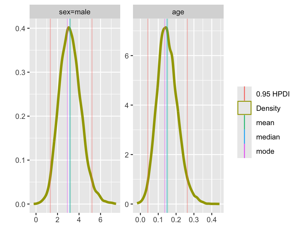
Code
plot(f, bivar=TRUE) # MAP region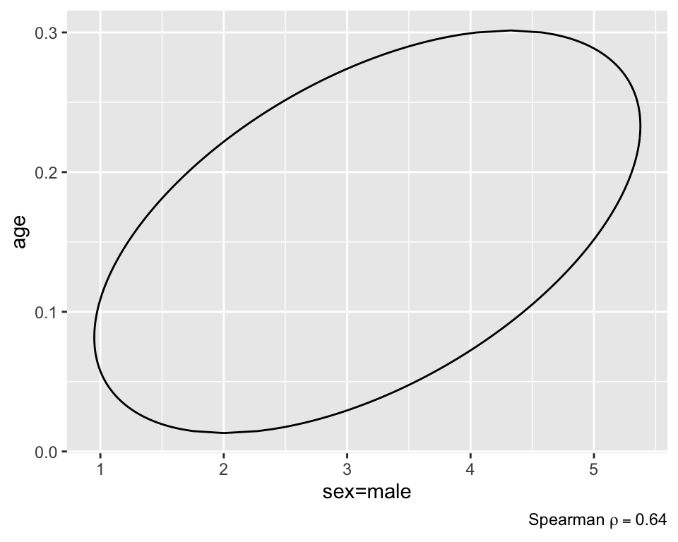
Code
plot(f, bivar=TRUE, bivarmethod='kernel')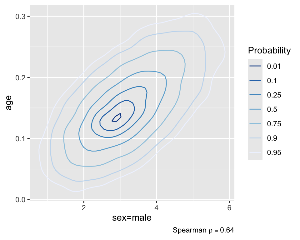
In the above figure, the point estimate does not appear quite at the point of highest density. This is because blrm estimates (by default) the posterior mean, rather than the posterior mode. You have the full posterior density, so you can calculate whatever you’d like if you don’t want the mean.
A plot of the partial effects on the probability scale from the Bayesian model reveals the same pattern as Figure 10.3 .
Code
# Partial effects plot
ggplot(Predict(f, age, sex, fun=plogis, funint=FALSE), ylab='P(Y=1)')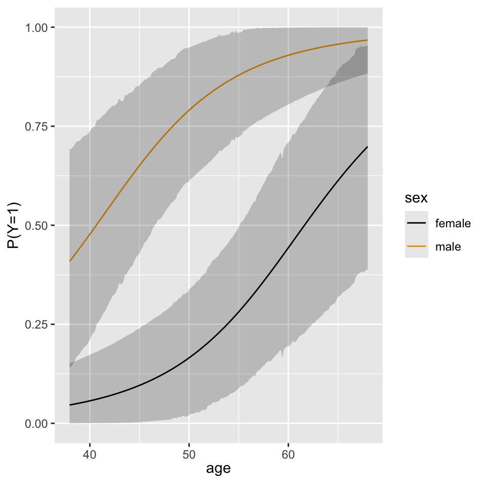
Code
# Frequentist
# variance-covariance for sex and age parameters
v <- vcov(flrm)[2:3,2:3]

# Sampling based parameter estimate correlation coefficient
f_cc <- v[1,2] / sqrt(v[1,1] * v[2,2])

# Bayesian
# Linear correlation between params from posterior
draws <- f$draws[, c('sex=male', 'age')]
b_cc <- cor(draws)[1,2]
Using the code in the block above, we calculate the frequentist sampling-based parameter estimate correlation coefficient is 0.75 while the linear correlation between the posterior draws for the age and sex parameters is 0.67. Both models indicate a comparable amount of correlation between the parameters, though in difference senses (sampling data vs. sampling posterior distribution of parameters).
Code
P <- PostF(f, pr=TRUE) Original Name Short Name
Intercept a1
sex=male b1
age b2 Code
(p1 <- P(b1 > 0)) # post prob(sex has positive association with Y)[1] 0.9999Code
(p2 <- P(b2 > 0))[1] 0.9985Code
(p3 <- P(b1 > 0 & b2 > 0))[1] 0.9984Code
(p4 <- P(b1 > 0 | b2 > 0))[1] 1The posterior probability that sex has a positive relationship with hospital death is estimated as \(\Pr(\beta_{sex} > 0)=0.9999\) while the posterior probability that age has a positive relationship with hospital death is \(\Pr(\beta_{age} > 0)=0.9985\) and the probability of both events is \(\Pr(\beta_{sex} > 0 \cap \beta_{age} > 0) = 0.9984\). Even using somewhat skeptical priors centered around 0, male gender and increasing age are highly likely to be associated with the response.
As seen above, the MCMC algorithm used by blrm provides us with samples from the joint posterior distribution of \(\beta_{age}\) and \(\beta_{sex}\). Unlike frequentist intervals which require the log-likelihood to be approximately quadratic in form, there are no such restrictions placed on the posterior distribution, as it will always be proportional to the product of the likelihood density and the prior, regardless of the likelihood function that is used. In this specific example, we notice that the bivariate density is somewhat skewed — a characteristic that would likely lead to unequal tail coverage probabilities if a symmetric confidence interval is used.
Code
ggplot(as.data.frame(draws), aes(x=`sex=male`, y = age)) +
  geom_hex() +
  theme(legend.position="none")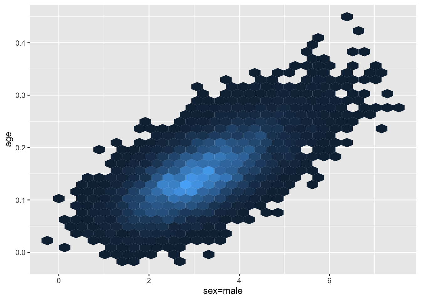
10.12 Study Questions
Section 10.1
- Why can the relationship between X and the log odds possibly be linear?
- Why can the relationship between X and the probability not possibly be linear over a wide range of X if X is powerful?
- In the logistic model Prob\([Y=1 | X] = \frac{1}{1 + \exp(-X\beta)} = P\), what is the inverse transformation of \(P\) that “frees” \(X\beta\), both in mathematical form and interpreted using words?
- A logistic model is used to relate treatment to the probability of patient response. X is coded 0 for treatment A, 1 for treatment B, and the model is Prob\([Y=1 |\) treatment\(]= \frac{1}{1+\exp[-(\beta_{0} + \beta_{1}X)]}\). What are the interpretations of \(\beta_{0}\) and \(\beta_{1}\) in this model? What is the interpretation of \(\exp(\beta_{1})\)?
- What does the estimate of \(\beta\) optimize in the logistic model?
- In OLS an \(F\) statistic involves the ratio between the explained sum of squares and an estimate of \(\sigma^2\). The numerator d.f. is the number of parameters being tested, and the denominator d.f. is the d.f. for error. Why do we always use \(\chi^2\) rather than \(F\) statistics with the logistic model? What denominator d.f. could you say a \(\chi^2\) statistic has?
- Consider a logistic model logit\((Y=1 | X) = \beta_{0} + \beta_{1}X_{1} + \beta_{2}X_{2}\), where \(X_1\) is binary and \(X_2\) is continuous. List all of the assumptions made by this model.
- A binary logistic model containing one variable (treatment, A vs. B) is fitted, resulting in \(\hat{\beta_{0}} = 0, \hat{\beta_{1}} = 1\), where the dummy variable in the model was I[treatment=B]. Compute the estimated B:A odds ratio, the odds of an event for patients on treatment B, and (to two decimal places) the probability of an event for patients on B.
- What is the central appeal of the odds ratio?
- Given the absence of interactions in a logistic model, which sort of subjects will show the maximum change in absolute risk when you vary any strong predictor?
- Would binary logistic regression be a good method for estimating the probability than a response exceeds a certain threshold?
Section 10.2
- What is the best basis for computing a confidence interval for a risk estimate?
- If subect risks are not mostly between 0-0.2 and 0.8-1.0, what is the minimum sample size for fitting a binary logistic model?
Section 10.5
- What is the best way to model non-additive effects of two continuous predictors?
- The lowess nonparametric smoother, with outlier detection turned off, is an excellent way to depict how a continuous predictor \(X\) relates to a binary response \(Y\) (although splining the predictor in a binary logistic model may perform better). How would one modify the usual lowess plot to result in a graph that assesses the fit of a simple linear logistic model containing only this one predictor \(X\) as a linear effect?
Section 10.8
- What are examples of high-information measures of predictive ability?
- What is a measure of pure discrimination for the binary logistic model? What commonly used measure in medical diagnosis is this measure equivalent to?
- Name something wrong with using the percent of correctly classified observations to quantify the accuracy of a logistic model.
Section 10.9
- What is the best way to demonstrate the absolute predictive accuracy of a binary logistic model?